Parallel Evaluation of Conjunctive Queries Paraschos Koutris
Dan Suciu
University of Washington Seattle, WA
University of Washington Seattle, WA
[email protected]
ABSTRACT The availability of large data centers with tens of thousands of servers has led to the popular adoption of massive parallelism for data analysis on large datasets. Several query languages exist for running queries on massively parallel architectures, some based on the MapReduce infrastructure, others using proprietary implementations. Motivated by this trend, this paper analyzes the parallel complexity of conjunctive queries. We propose a very simple model of parallel computation that captures these architectures, in which the complexity parameter is the number of parallel steps requiring synchronization of all servers. We study the complexity of conjunctive queries and give a complete characterization of the queries which can be computed in one parallel step. These form a strict subset of hierarchical queries, and include flat queries like R(x, y), S(x, z), T (x, v), U (x, w), tall queries like R(x), S(x, y), T (x, y, z), U (x, y, z, w), and combinations thereof, which we call tall-flat queries. We describe an algorithm for computing in parallel any tall-flat query, and prove that any query that is not tall-flat cannot be computed in one step in this model. Finally, we present extensions of our results to queries that are not tall-flat.
Categories and Subject Descriptors H.2.4 [Systems]: Distributed Databases
General Terms Algorithms, Theory
Keywords Database Theory, Distributed Databases, Parallel Computation
1. INTRODUCTION In this paper we study the parallel complexity of conjunctive queries. Our motivation comes from the recent increase ∗ This work was partially supported by NSF IIS-0627585 and IIS-0713576.
Permission to make digital or hard copies of all or part of this work for personal or classroom use is granted without fee provided that copies are not made or distributed for profit or commercial advantage and that copies bear this notice and the full citation on the first page. To copy otherwise, to republish, to post on servers or to redistribute to lists, requires prior specific permission and/or a fee. PODS’11, June 13–15, 2011, Athens, Greece. Copyright 2011 ACM 978-1-4503-0660-7/11/06 ...$10.00.
∗
[email protected]
in the use of massive parallelism for performing data analysis on very large datasets. In addition to traditional parallel database systems, such as Teradata or Greenplum, new query languages and implementations have been introduced recently for the purpose of massively parallel data analytics: the MapReduce architecture for parallelism [8], SCOPE [4], DryadLINQ [25], Pig [10], Hive [22], Dremel [17]. Most of the effort and the engineering work in these systems has been focused on fault-tolerance, resource allocation, and scheduling, and restricted to basic operations like filtering, groupby, aggregation, and join. As these systems evolve towards general-purpose data analytics languages, they need to optimize and execute in parallel general conjunctive queries. The parallel complexity of conjunctive queries on today’s parallel architectures is not well understood. The data complexity of every relational query is in AC0 [16], and it is generally acknowledged that SQL is “embarrassingly parallel”. Immerman [13] analyzed the parallel complexity of First Order Logic on CRCW PRAM (Concurrent Read, Concurrent Write Parallel Random Access Machine) [21] and showed that the parallel time is equivalent to the number of times one needs to iterate a First Order sentence; an immediate corollary is that every relational query takes O(1) parallel time in this model. But circuits and PRAMs are not accurate models of parallel systems. Even in the 80’s and 90’s researchers have proposed alternative models to capture parallelism. Valiant introduced the BSP model [23] and Culler et al. further refined it into the LogP model [6]. Both view the parallel computation as a sequence of relatively short parallel computation steps, each followed by a global synchronization barrier. The length of a parallel step is called periodicity parameter, L, and most of the analysis of parallel algorithms in these models consists of theoretical guarantees that servers finish their tasks within the periodicity parameter (or else, the next step needs to be dedicated to the unfinished step). Therefore, the models focus on the details of the communication protocol, and trace meticulously the network’s latency, overhead, and gap (in the LogP model). These models no longer capture today’s parallel architectures well. Nowadays, massive parallelism is achieved on commodity hardware interconnected by a high speed network. The communication cost is less dependent on the low level protocol, but is dominated by the amount of data being exchanged. In addition, the granularity of a parallel step has increased, since each server needs to process a large amount of data before synchronization, making each synchronization step even more expensive. The main bottleneck in today’s massively parallel computations is the global synchronization steps of a computation [12]. Two factors make a global synchronization step
expensive: data skew and stragglers. Data skew refers to the fact that some servers end up processing much more data than others. Theoretically, one addresses data skew by requiring that each server is allocated only O(n/P ) of the total data, where n is the number of data items and P the number of servers. This guarantees that no server gets an excessive load1 . Stragglers are a new phenomenon, not encountered in older parallel systems. A straggler is a server that takes significantly longer time to execute its share of the computation than the others. This can be caused by a faulty disk, the server being overloaded with other tasks, by server failure, or by the algorithm itself. Stragglers occur in today’s systems because the large number of servers (tens of thousands) and the long processing times (often several hours) dramatically increase the probability that some servers will straggle. All systems to date, starting with the original MapReduce [8], pay special attention to stragglers. They monitor slow responders, and, once a straggler is identified, its work is redistributed to other servers. Despite these measures, stragglers add a significant cost to each synchronization step, and the way to mitigate that cost in a theoretical model is to reduce the number of global synchronization steps. We propose a simple parallel model of computation, called the Massively Parallel, or MP model, to enable us to analyze the parallel complexity of conjunctive queries. In MP, computation proceeds in a sequence of parallel steps, each followed by global synchronization of all servers. We do not impose any restriction on the time of a parallel step. Instead, we impose the restriction that the load at each server is no more than O(n/P ) data items during the entire computation, where n is the total size of the input and the output, and P is the number of servers. Each parallel step consists of a broadcast phase (where a limited amount of data is shared among servers, typically in order to detect skewed elements), followed by a communication phase, followed by a computation phase. The cost of an algorithm in the MP model is given by the number of parallel steps: we ignore the time of the computation phase and also, in this paper, we ignore the total amount of data transferred during communication. However, notice that the amount of data transferred is always O(n), because the P processors can receive at most P · O(n/P ) data items during each communication step; this is in contrast √ to Afrati and Ullman [1], who allow k a total amount of O(n P k−1 ) data exchanged in one step (see Section 7). Thus, we only count the number of synchronization steps. For example, if Algorithm A computes a query in two parallel steps, each taking time T , and Algorithm B computes the same query in a single parallel step of time T ′ = 2T , then both algorithms take time 2T , and would be considered equivalent in a traditional model. But, under MP, Algorithm B is better, since it uses one parallel step instead of two. In this paper we study the evaluation of conjunctive queries in the MP model. We restrict our discussion to full conjunctive queries (without projections). Our main result is a complete characterization of queries computable in one MP step; the most significant aspect of this result is that not all queries are easily parallelizable, as older models of parallelism suggest. The queries computable in one MP step are the tall-flat queries. A flat query is one where every two atoms share the same sets of variables, for example q(x, y, z, u) = R(x, y), S(x, z), T (x, u) is flat because 1
We assume that each of the n items takes about the same time to process. This assumption may fail for jobs with user defined functions.
any two atoms share {x}; in other words, a flat query is a star join where all join conditions are on the same variable(s). A tall query is one where the set of variables in the atoms forms a linear chain, for example q(x, y, z, u) = R(x), S(x, y), T (x, y, z), U (x, y, z, u); tall queries occur in data warehouse schemas, e.g Country(co, ...), City(co, ci, . . .), Store(co, ci, st, . . .). A tall-flat query consists of a tall part followed by a flat part (formal definition in Section 3), and we prove that a query can be evaluated in one MP step iff it is tall-flat. For the “if” part of the proof, we give a concrete algorithm that computes any tall-flat query in one parallel step, while guaranteeing perfect load balance (which is a requirement in the MP model), even if the data is skewed. We give the algorithm in two stages: we describe the algorithm separately for tall, and for flat queries in Section 4, then combine them into a general algorithm in Section 5. The simple case of a 2-way join q(x, y, z) = R(x, y), S(y, z) can be computed by an alogorithm similar in spirit to the skew join in Pig [10]; k-way flat queries with k ≥ 3 and tall queries require non-trivial extensions. For the “only if” part of the proof, we show in Section 6 that for any non tall-flat query, any one-step parallel algorithm will be skewed, thus violating the MP model. Our results depend critically on the load balance requirement, which strictly limits the amount of data per processor to O(n/P ), and, hence, limits the communication cost to O(n). Afrati and Ullman [1] describe a simple algorithm for computing the query RST (x, y) = R(x), S(x, y), T (y) (which is not tall-flat)√in one parallel step, by allowing each server to store O(n/ P )√amount of data, and, thus, with communication cost O(n P ). In general, any conjunctive query with k variables can be computed in one parallel √ step if one allows the load per processor to√increase to O(n/ k P ) k (and the communication cost to O(n P k−1 )). Organization. We first discuss in Section 2 about related work in parallel and distributed database models. Then, we describe the model and the main algorithmic techniques in Section 3, and the main algorithms in Section 4. We prove the main result in Section 5 and Section 6. Finally, we discuss some extensions in Section 7 and conclude in Section 8.
2.
RELATED WORK
The recent success of the MapReduce framework [8] in efficiently parallelizing computations has inspired theoretical research on new models of parallel computation, which capture the characteristics and limitations of the new architecture, while also considering the capabilities of modern hardware and infrastructure. Afrati and Ullman [1] describe a model of computation where every query is executed in one parallel step and the primary measure of complexity is communication. Our model always restricts the communication to O(n), but needs multiple communication steps, hence this is our main complexity metric. By contrast, in their work they allow a larger √ k amount of communication, typically O(n P k−1 ), and therefore the main complexity metric is the total amount of communication. Another theoretical approach to analyzing MapReduce is presented in [14]. In this paper, the authors allow only a limited amount of storage in each processor, and add randomization, in the sense of allowing false computations as well. Their main measure of complexity is similar to ours: the number of MapReduce steps; however, they do not examine queries, but general algorithms, comparing their model to the PRAM model.
Measuring parallel complexity in terms of the the number of communication steps was also proposed by Hellerstein [12], who introduced the notion of Coordination Complexity. The author argues that both communication and computation are cheap using today’s infrastructure; the bottleneck in parallelizing queries lies in the coordination of global barriers during computation. Apart from recent approaches to modeling the MapReduce framework, various parallel models have been extensively studied, for example the widely used bulk-synchronous parallel model [23] and the LogP model [6]. However, both models do not seem to adequately capture the concerns of today’s massively parallel computations. The idea that we handle skewed elements in a special way during computation is not a new one; in [24], the authors develop and implement an algorithm similar to ours that handles skewed join computation in shared-nothing architectures. Nevertheless, they assume that they have knowledge of the skewed elements and do not provide any theoretical guarantees on their algorithm. Grohe et al. [11] introduced the Finite Cursor Machines model of computation, in which queries are evaluated in a sequence of “streaming” steps: each relation can be sorted at the beginning of the step, but afterwards can be read a constant number of times using a constant amount of memory, in a streaming fashion. They do not restrict to full queries, but they do restrict to conjunctive queries in the semi-join algebra in order to ensure that the output is linear in the size of the input (this rules out cartesian product queries like q(x, y) = R(x), S(y)). For example, a query like q(x) = R(x, y), S(x, z), T (x, u) can be computed in one step, by first sorting the relations on x, then mergejoining the three streams. The authors prove that the query q(x, y) = R(x), S(x, y), T (y) cannot be computed in one streaming step in this model. A conjunctive query is called hierarchical if, denoting at(x) the set of atoms that contain the variable x, the family of sets {at(x) | x ∈ V ar(Q)} form a hierarchy (formal definition in Subsection 3.1). Although the authors [11] do not state this explicitly, it follows immediately from their result that a conjunctive query in the semi-join algebra can be evaluated in one step iff it is hierarchical. Dalvi et al.[7] show that, over tuple-independent probabilistic databases, queries that can be evaluated efficiently are precisely the hierarchical queries 2 . Thus, both in the streaming and probabilistic data model, the tractable queries have the property of being hierarchical. In our work we consider full conjunctive queries, but do not restrict to the semi-join algebra. Thus, we allow cartesian product queries, and show that the queries computable in one pass are the tall-flat queries: for example the cartesian product query q(x, y) = R(x), S(y) is flat, and therefore computable in one MP step. Yet, not every hierarchical query is tall-flat, for example q(x, y) = R(x), S(x), T (y), and these cannot be computed in one MP step (Section 6). When restricting to queries that are both full and in the semi-join algebra of [11], we prove that hierarchical queries coincide with tall queries and tall-flat queries collapse to tall queries [15]. Thus, for the intersection of the language considered in [11] and the one in this paper, the class of “easy” queries coincides.
3. THE MODEL AND THE MAIN RESULT We define here the Massively Parallel (MP) model of query evaluation. We fix throughout this paper a domain, U , 2 This result applies only to conjunctive queries without selfjoins.
called universe. A relational database instance D contains constants from U , and has a relational schema R = R, S, T, . . . We consider in this paper only full conjunctive queries, i.e. where all variables are head variables. Denote the problem size to be the size of the input database plus the size of the query’s answer, n = size(D) + size(Q) . Let P be the number of parallel servers. Each server stores two kinds of data: generic data (values from U ) and numerical data (integers). The data is stored in arrays, on disks or in main memory. Generic values can be manipulated only in three ways: they can be copied, they can be tested for equality a = b, and they can be subjected to a hash function, ¯ Each hash function has from a fixed set of hash functions h. type h : U k → [P ], where k is its arity. For example, an ¯ = (h1 , h2 , h3 ), algorithm may use three hash functions, h 3 where h1 , h2 : U → [P ] and h3 : U → [P ]. Each hash function is randomized at the beginning of the algorithm, i.e. chosen randomly from a finite set3 H of a family of hash functions 4 . Initially, all relations are already uniformly distributed over the servers (so no additional communication is necessary), and their sizes are known by all servers. An algorithm in the MP model runs as follows. The input is the database instance D. Each relation R is partitioned into P fragments R1 , R2 , . . . , RP of equal size, and distributed over the P servers; server s holds the fragments Rs , Ss , Ts , . . . The initial load of each server is size(D)/P . The algorithm proceeds in a number of parallel computation steps, each consisting of three phases: Broadcast Phase: The P servers exchange some data globally. This data is shared among all servers, and we call it broadcast data, B. At the end of this phase each server has a copy of B. We require the total amount of communication in this phase to be O(nε ), for some 0 < ε < 1; in particular, size(B) = O(nε /P ). Communication Phase: Each server sends data to other servers. There is no restriction imposed on how a server distributes the data to the other servers; it could send its entire data to a single server, distribute it uniformly among servers, or broadcast its entire data to all servers (but see the skew-free requirement below). Computation Phase: Each server performs some local computation on its data. There is no restriction imposed on the time taken for the computation. At the end of this phase the algorithm may stop and leave the result in the local memory of the P servers, or may continue with the next parallel step. We allow local computation to be performed during all three phases; in our model local computation is free. A parallel algorithm is a sequence of parallel computation steps, and its cost is the number of parallel steps. Let ns denote the total number of tuples stored at sever s during the entire execution of the algorithm. The algorithm is called load balanced, or skew free, if, for sufficiently large n, E[maxs ns ] = O(n/P ), where the expectation is taken over ¯ ∈ H. Formally: the random choices of the hash functions h 3 Strictly speaking, we need a separate family for each hash function used: h1 ∈ H1 , h2 ∈ H2 , etc. To simplify things, ¯ ∈ H with some abuse. we use a single family and write h 4 Although in this paper we allow randomization only in the choice of hash functions (with the exception of Subsection 4.1), all the hardness results (apart from Proposition 4.3, which we defer to the full version) easily extend to arbitrary use of randomization.
Definition 3.1. An algorithm is load balanced if there exists a constant factor c > 0 s.t. for all number of servers P there exists an integer n0 such that size(D) = n ≥ n0 , implies Eh∈H [maxs=1,P ns ] ≤ c · n/P . ¯ We require every algorithm to be load balanced. This requirement is a key element of the MP model. Without it, any query could be computed in one step, because all servers could send their data to server number 1, which computes the query locally. It has two consequences. First, it ensures linear speedup [9] (by doubling the number of servers P , the load per server will be cut in half5 ) and constant scaleup (by doubling both the size of the data n and the number of processors P , the running time remains unchanged). Second, it implies that the total amount of data exchanged during each communication step is O(n) in expectation. Indeed, let ns be the number of tuples received by server s = 1, P : sinceP E[ns ] = O(n/P ), the total amount of data exchanged is E[ s ns ] = O(n). Thus, the amount of communication is guaranteed to be O(n). In most algorithms, this is also a lower bound, but in some cases one can design algorithms with strictly less communication. For example, consider the intersection query q(x) = R(x), S(x); partitioned hash join has communication cost n = |R| + |S| (Proposition 3.3). But if we know that |R| ≪ |S|, then we can use broadcast join: broadcast R to all servers, then each server intersects R with its local fragment of S. The communication cost is P · |R|, which may be much less than n. In this paper, we do not distinguish between these two algorithms, since both require one parallel step. The MP model is related to, but not identical to a Map Reduce (MR) job [8]. MR corresponds to one MP step: there is no broadcast phase, the communication phase is the map job followed by data reshuffling, and the computation phase is the reduce job. However, to implement an MP algorithm over MR one has to implement the broadcast phase either as a separate, lightweight MR job, or by sampling the data before it is partitioned into servers at the beginning of the map job. As we show in Proposition 3.5, the broadcast phase is necessary to ensure load balance even for the simplest of the join algorithms, and this is why we include it in the model. Using sampling in order to improve load balance is a popular technique in practice, for example it is used in skew join in Pig [10]. Finally, note that in Definition 3.1, n0 is allowed to depend on P . In other words, once P is fixed, load balance is expected only for n “large enough”. In some of our algorithms we require P = O(nε ), for some 0 < ε < 1.
3.1 Main Result The main result in this paper is a complete characterization of queries that are computable in one MP step by a load balanced algorithm. To describe this result we first need some definitions. Given a conjunctive query Q and a variable x, denote by at(x) the set of atoms that contain x. A query is called hierarchical if for any two variables x, y, one of the following holds: at(x) ⊆ at(y) or at(x) ⊇ at(y) or at(x) ∩ at(y) = ∅. A conjunctive query is called tall-flat if one can order its variables x1 , . . . , xk , y1 , . . . , yℓ such that: (1) at(x1 ) ⊇ at(x2 ) ⊇ . . . ⊇ at(xk ), (2) at(xk ) ⊇ at(yi ) for i = 1, . . . , ℓ, and (3) |at(yi )| = 1. Clearly, every tall-flat query is hierarchical. Furthermore, if l = 0 then we call it a tall query, and 5
And, thus, the time of the computation phase will also be halved, assuming that the computation time is linear in the size of the data.
y1 x1
x2
x3
x4
y2 y3
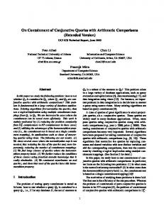
Figure 1: The tall-flat query L. An arrow u → v denotes that at(u) ⊆ at(v). if k = 1 then we call it a flat query. For example the query L(x1 , x2 , x3 , x4 , y1 , y2 , y3 ) : − R1 (x1 ), R2 (x1 , x2 ), R3 (x1 , x2 , x3 ), R4 (x1 , x2 , x3 , x4 ), S1 (x1 , x2 , x3 , x4 , y1 ), S2 (x1 , x2 , x3 , x4 , y2 ), S3 (x1 , x2 , x3 , x4 , y3 ) is a tall-flat query (Figure 1). The main result we prove is: Theorem 3.2. Every tall-flat conjunctive query can be evaluated in one MP step by a load balanced algorithm. Conversely, if a query is not tall-flat, then every algorithm consisting of one MP step is not load balanced.
3.2
Datalog Notation for MP Algorithms
Throughout the paper, we express algorithms using a simple extension to non-recursive datalog, which allows us to specify the location where data is stored. For this purpose we adopt the syntax from [2]. If R(x, y) is a relation (binary in this case), then the notation R(@s,x,y) denotes the fragment of the relation R which is stored at server s. Using this notation, we can define computations and communication in the following way: • Local computation: R(@s,x,y):-S(@s,x,y),T(@s,x) • Broadcast: R(@*,x):-S(@s,x),T(@s,x) • Point-to-point communication: R(@h(x),x,y):-S(@s,x,y)
3.3
Examples
We illustrate our model by giving two simple algorithms, for computing the intersection of two sets, and a semijoin. The first query computes the intersection of two sets R, S, Q(x) : −R(x), S(x). This query is both tall and flat, and can be computed by the distributed hash-join Algorithm 1. Algorithm 1: Intersection(R(x), S(x)) /* Communication Phase */ R2(@h(x), x) :- R(@s, x) S2(@h(x), x) :- S(@s, x) /* Computation Phase */ Q(@s, x) :- R2(@s, x), S2(@s, x)
In this algorithm, h is a hash function h : U → [P ]. Each server s applies the hash function h to each tuple R(a) and sends it to the destination server h(a); similarly for tuples S(b). In the computation phase, the tuples placed in the same server are joined. Clearly, this algorithm is correct, and runs in one parallel step, having no broadcast phase. We will prove next that it is load balanced. No fixed hash function h can guarantee load balance, because there exists a worst case data instance such that all its data values collude under h. Instead, we follow here the
standard approach, and assume that h is a uniform family 6 of hash functions [18]. Thus, in general, any MP algorithm starts by choosing randomly its hash functions from ¯ ∈ H are made, we call the execution H: once these choices h of the algorithm a run. The load balance requirement can be rephrased as follows: Eh∈H [maxs ns ] = O(n/P ), where ¯ the expectation is taken over all runs. Proposition 3.3. Assuming n = Ω(P log P ), Algorithm 1 is load balanced, i.e. the expected maximum server load is E[maxs ns ] = O(n/P ). Proof. Consider the classical balls in bins problem: n balls are randomly thrown into P bins. If n = Ω(P log P ), the expected maximum load of a bin is Θ(n/P ) [19]. This immediately proves the claim: each of the n tuples in R and S is a ball, and h places each tuple independently in one of the P servers (= bins), because h is chosen from a uniform family of hash functions, hence E[maxs ns ] = Θ(n/P ). Our second example illustrates the broadcast phase. Consider the query Q(x, y) : −R(x), S(x, y): this is a semijoin, and it is a tall query. A naive extension of the previous algorithm would partition both R(x) and S(x, y) according to a hash function h(x), but this may result in data skew: for example, if all tuples S(x, y) have the same value x = a, then they will be hashed to the same server h(a), whose load increases to O(n). Here it is necessary to obtain some information about the distribution of tuples in S, using the broadcast phase. Algorithm 2 performs a load balanced computation of the semijoin query. Algorithm 2: Semi-join(R(x), S(x, y)) /* Broadcast Phase */ /* Compute skewed elements; τ = |S|/(P log P ) */ G(@s, x, count(*)) :- S(@s,x,y) H(@s, x) :- G(@s,x,f), f > τ /P B(@*, x) :- H(@s, x) /* Broadcast */ /* Communication Phase */ R2(@h(x), x) :- R(@s, x), not B(@s, x) S(@h(x), x, y) :- S(@s, x, y), not B(@s, x) R2(@*, x) :- R(@s, x), B(@s, x) S(@h2(x,y), x) :- S(@s, x, y), B(@s, x) /* Computation Phase */ Q(@s, x, y) :- R2(@s, x), S2(@s, x, y) In general, for any relation S(x, . . .) and attribute x of S, define the frequency fS,x (a) of a constant a to be the number of elements in S that have a on the x position. Let τ > 0 be a value called a threshold. A value a is called (S, x, τ )skewed, or simply skewed, or frequent, if fS,x (a) ≥ τ ; we denote FS,x,τ (x) the set of skewed elements. Notice that |FS,x,τ | ≤ |S|/τ . The semi-join Algorithm 2 starts by computing all τ -skewed elements, for τ = |S|/(P log P ). This set cannot be efficiently computed exactly, because S is distributed; instead we compute a superset B. Each server s computes all elements x whose local frequency is ≥ τ /P ; the count(*) notation is from [5]. There are ≤ (|S|/P )/(τ /P ) = |S|/τ locally skewed elements. These sets are broadcast, and each server computes their union, B. The set B contains FS,x,τ , 6 The family H is called uniform on a set S = {x1 , . . . , xk } if h ∈ H maps S to k values that are uniformly random and independent. Uniformity is strictly stronger than universality [3]. In all our algorithms, |S| = O(n).
and |B| ≤ P · |S|/τ ; thus the communication cost of the broadcast phase is ≤ P 2 · |S|/τ = P 3 log P = O(nε ) (we show in Subsection 4.1 how to further improve this). Next, the semi-join algorithm proceeds as follows. For all nonskewed elements x, both R(x) and S(x, y) are sent to the server h(x); for the skewed elements, S(x, y) is distributed using a second hash function h2(x, y), while R(x) is broadcast to all servers. This is similar to skew join in Pig [10], but computes the skewed elements differently. Proposition 3.4. Assuming n = Ω(P 3 log P ), Algorithm 2 is load balanced. The proof follows as a corollary of Theorem 4.4, which we prove in the next section. We now prove that, without a broadcast phase, no loadbalanced algorithm can compute the semi-join in one step. This justifies including a broadcast phase in the MP model. Proposition 3.5. If an algorithm for computing the semijoin Q(x, y) : −R(x), S(x, y) has one single parallel step and no broadcast phase, then it is skewed. Proof. We start by revisiting how the data is partitioned. In the MP model the input data is partitioned jointly: each sever holds a fragment from each relation. But in impossibility proofs we will assume that the database is partitioned separately: each server holds a fragment from only one relation: P · |R|/(|R| + |S|) severs hold fragments of R, and P · |S|/(|R| + |S|) servers hold fragments of S. Any impossibility result for the separate partition implies an impossibility result for the joint partition, because any load balanced algorithm A over the separate partition can be simulated by a balanced algorithm A′ over the joint partition as follows. Given a separately partitioned instance R, S, extend it to a joint partitioned instance R′ , S ′ , by inserting new R-tuples in the servers holding S, and inserting new S-tuples in the servers holding R, such that |R′ | = |S ′ | = |R| + |S|. The new tuples are chosen s.t. they do not join with any other tuples. Run A′ on R′ , S ′ : the result is S ′ ⋉ R′ = S ⋉ R. Thus, w.l.o.g., we will assume a separate partition in all impossibility proofs. Assume A is a load balanced algorithm computing the query Q. Let c be the constant in Definition 3.1, let P ≥ 64c2 , and let n = n0 , where n0 is given by Definition 3.1 (it may depend on P ). We will show that A does not compute correctly Q on an instance of size 2n using P processors. To simplify the notations we assume that A uses a single hash function h, of arity k: the extension to multiple hash functions is straightforward. Fix two n-vectors X = (x1 , . . . , xn ) and Y = (y1 , . . . , yn ) ∈ U n of distinct elements. For each m = 1, n, denote D(m) = (R, S (m) ) the instance R = {x1 , . . . , xn }, and S (m) = {(xm , y1 ), . . . , (xm , yn )}. For any run h ∈ H, let Kh (R(xi )) and Kh (S(xi , yj )) ⊆ [P ] be the set of servers that receive R(xi ) or S(xi , yj ) respectively. Lemma 3.6. If A is load balanced, then for any X, Y ∈ U n , there exists an instance D(m) (constructed from X, Y, m as explained above), a run h ∈ H, and an element yi ∈ Y , such that Kh (R(xm )) ∩ Kh (S(xm , yi )) = ∅. Proof. Let ns (D(m) , h) be the load at server s for the instance D(m) and the run h. Since size(D(m) ) = 2n, by Definition 3.1, Eh∈H (maxs ns (D(m) , h)) ≤ 2·c·n/P . Let d = 4·c. We say that h is balanced for D(m) if maxs (ns (D(m) , h)) ≤ 2 · d · n/P , and we say that h is balanced if it is balanced for some D(m) . Denote by H(m) the set of runs balanced
S for D(m) , and H(∗) = m H(m) . By Markov’s inequality, (m) |H |/|H| ≥ 1 − c/d = 3/4, and also |H(∗) |/|H| ≥ 3/4: thus, most runs are balanced. Call an element xi good for run h if, on some input D(m) , |Kh (R(xi ))| < P/(2 · d): “goodness” does not depend on D(m) , because the input is partitioned separately, and all instances D(m) have the same R. We claim that there exists m such that xm is good for some h ∈ H(m) . The claim proves the lemma: indeed, consider the run h on the instance D(m) . Each server in Kh (R(xm )) stores at most 2 · d · n/P tuples (since h is balanced for D(m) ); hence, together they hold < P/(2 · d) × 2 · d · n/P = n tuples. This implies that at least one of the n tuples S(xm , yi ), i = 1, n is not sent to any server in Kh (R(xm )). To prove the claim, denote for each h ∈ H(∗) : Bh ={xi | |Kh (R(xi ))| ≥ P/(2 · d)}
Gh ={xi | |Kh (R(xi ))| < P/(2 · d)}
(bad elements)
(good elements)
Clearly, Bh ∪ Gh = {x1 , . . . , xn }. Since h is balanced for some D(m) we have |Bh | · P/(2 · d) ≤ 2 · d · n. Therefore:
4d2 ) × n ≥ 3/4 · n ∀h ∈ H(∗) (1) P The last inequality holds because P ≥ 64c2 = 16d2 . We now prove that there exists a set H′ ⊆ H(∗) such that: T and |H′ | ≥ 3/4 · |H(∗) | ≥ 9/16 · |H| (2) h∈H′ Gh 6= ∅ |Gh | ≥(1 −
For that, consider the {0, 1}-matrix E = (eih ) of dimensions n × |H(∗) |, where eih = 1 iff xi ∈ Gh . By Equation 1, every column h has at least 3/4 of entries equal to 1; thus, at least 3/4 of entries in the entire matrix are 1; thus, there exists a row m with at least 3/4 of the entries 1. Then, H′ = {h | emh = 1} satisfies Equation 2. To prove the claim, we show that H(m) ∩ H′ 6= ∅. This follows from |H(m) | + |H′ | ≥ 3/4 · |H| + 9/16 · |H| = 21/16 · |H|: the two sets combined have more elements than H and therefore have a non-empty intersection.
Fix D = D(m) = (R, S (m) ), and the run h given by the lemma. We will show that the algorithm is incorrect on the run h, by showing that it fails to output the tuple (xm , yi ). Servers 6∈ Kh (S(xm , yi )) cannot output this tuple, since they don’t receive yi and cannot fabricate a generic value in U . Servers ∈ Kh (S(xm , yi )) don’t receive R(xm ). To show that they cannot output this tuple either, consider the execution of the algorithm on a second instance D′ = (R′ , S (m) ) where R′ is obtained from R by replacing the single tuple R(xm ) with R(x′m ), where x′m 6= xm : (x′m , yi ) is no longer an answer to Q on D′ . Servers holding input fragments of S will send their data to the same destinations, since S is unchanged; in particular, S(xm , yi ) is sent to the same set Kh (S(xm , yi )). We claim that, during the two execution of the algorithm, on D and D′ respectively, the server holding R(xm ) (in D) or R(x′m ) (in D′ ) will obtain exactly the same hash values; in particular, it will send its elements to exactly the same destinations, hence Kh (R(x′m )) ∩ Kh (S(xm , yi )) = ∅. Thus, the servers in Kh (S(xm , yi )) receive exactly the same elements during the two executions, and will not be able to distinguish between D and D′ , thus cannot determine whether to output the tuple (xm , yi ). It remains to prove the claim. For X ∈ U n denote H(X) the array consisting of all hash functions h ∈ H applied to all values in X. One can view H as assigning a color to each point in U n . The number of colors is finite, c: for example, if all hash functions in H have type h : U k → [P ], then k c = [P ]|H|·n . Call a set V¯ = V1 × · · · × Vn ⊆ U n a p-space if
|Vi | ≥ p, for i = 1, n. A p-space is unicolored if all its points have the same color. We prove that there exists a unicolored 2-space {x1 , x′1 } × · · · × {xn , x′n }. This implies Corollary 3.8, which proves the claim. Lemma 3.7. Suppose all points in U n are colored with c colors. Then, for every p > 0 there exists M > 0 such that every M -space has a unicolored p-subspace. In particular, if U is infinite, then U n has a unicolored 2-subspace. Proof. We set M = fn (p), where f1 (p) = (p − 1) · c + 1, (f (p)) (k) fn+1 (p) = fn 1 (p) (where fn (p) = fn (· · · fn (p) · · · ), k times). The proof is by induction on n. For n = 1, consider a set V1 with f1 (p) points: at least p have the same color. Assuming the lemma is true for n, we prove it for n + 1. Let M = fn+1 (p) and consider an (n + 1)-dimensional M -space V¯ 0 × Vn+1 , where V¯ 0 = V1 × · · · × Vn . Let k = (p − 1) · c + 1. Fix k distinct elements x1 , . . . , xk ∈ Vn+1 (this is possible since |Vn+1 | ≥ M = fn+1 (p) ≥ f1 (p) = k). Denote pk = p, pi−1 = fn (pi ) for i = k, . . . , 1; thus, M = p0 . For every i = 1, k there exists an n-dimensional pi -space V¯ i such that V¯ i × {xi } is unicolored, and V¯ i ⊆ V¯ i−1 : indeed, V¯ 0 × {x1 } is an n-dimensional space, hence by induction on n has a unicolored subspace V¯ 1 × {x1 }; suppose V¯ i−1 × {xi−1 } is unicolored: since V¯ i−1 ×{xi } is an n-dimensional pi−1 -space, it has a unicolored pi -subspace V¯ i × {xi }. Thus, we obtain k unicolored spaces, V¯ 1 × {x1 }, . . . , V¯ k × {xk }, and at least p of them have the same color: V¯ i1 × {xi1 }, . . ., V¯ ip × {xip }. Then V¯ ip × {xi1 , . . . , xip } is a unicolored p-space. Corollary 3.8. There exist vectors X = (x1 , . . . , xn ) and Y = (x′1 , . . . , x′n ) such that for any m, the vectors X and X ′ = (x1 , . . . , x′m , . . . , xn ) collude.
4.
THREE BUILDING BLOCKS
In this section, we describe the building blocks for the algorithm computing any tall-flat query in one MP step: we give an algorithm for computing the frequent elements of a relation, an algorithm for computing any flat query, and an algorithm for computing any tall query. In Section 5 we combine them to give a general algorithm for any tall-flat query.
4.1
Computing High Frequency Elements
The distributed frequent elements problem is the following: given a distributed relation R(x, . . . ) of size r = |R|, and a threshold τ , compute a set F containing all skewed elements FR,x,τ , and distribute F to all servers. We consider algorithms that proceed in two steps: (a) compute and broadcast a set B to all servers, and (b) compute a subset F of B at each server s.t. F is a superset of FR,x,τ . We define two costs: the amortized communication cost, |B|, and the excess cost, |F |. Our goal is to keep the amortized cost O(nε /P ), becuase the total communication cost is P · |B|. The excess is at least r/τ , because, in the worst case, there are r/τ frequent elements FR,x,τ : our goal is to prevent it from being much larger. We present here three algorithms for the distributed frequent element problem. The naive algorithm consists of the top three rules in Algorithm 2. Here F = B, hence both amortized cost and excess are ≤ P · r/τ . The Deterministic Frequency, Algorithm 3, has essentially the same amortized cost, but a smaller excess. It starts by computing all elements whose local frequency is ≥ τ /(2P ), and retains their local frequencies, then broadcasts these elements: thus, the amortized communication cost is |B| ≤
Algorithm 3: Deterministic Frequency(R, τ ) HS(@s,x,count(*)):- R(@s,x,...) G(@s,x,f) :- HS(@s,x,f), f > τ /(2P ) B(@*,x,f,s) :- G(@s,x,f) /* Broadcast */ H(@s,x,sum(*)) :- B(@s,x,f,-) F(@s,x) :- H(@s, x, f), f ≥ τ /2 2 · P · r/τ , twice that of the naive algorithm. Then, it retains in F only those elements x whose total frequency exceeds τ /2; therefore, the excess is |F | ≤ 2 · r/τ , a factor of P/2 smaller than the naive algorithm. Algorithm 4: Frequency Sampling(R, τ ) T = c · r · log r/τ /* c is a constant */ ts ∼ B(r, T /(P · r)) /* binomial sample */ H(@s, x, ...) :- sampling(@s, R, ts ) G(@s, x, count(*)) :- H(@s, x, ...) B(@*, x, s) :- H(@s, x, ...) /* Broadcast */ K(@s, x, count(*)) :- B(@s, x, -) F(@s, x) :- K(@s, x, f), f ≥ c · τ · T /r The Frequency Sampling, Algorithm 4, has both a smaller amortized communication, and a smaller excess cost over the naive algorithm. Denote T = c · r · log r/τ , where c > 0 is some constant. The algorithm starts by computing a “coinflip” sample B of R, where each element of R is sampled independently, without replacement, with probability T /r. Thus, E[|B|] = T , and the amortized communication cost is c · r · log r/τ in expectation, which is significantly lower than P · r/τ when log r ≪ P . To compute B distributively, each server s generates a random number ts drawn from a binomial distribution B(r, T /(P · r)) (thus, E[ts ] = T /P ), then samples ts elements without replacement from its local fragment Rs , using the primitive function sampling(@s, R, ts ). Once B has been computed and broadcast, we retain in F only those elements whose total frequency is ≥ c · τ · Tr . We prove in the appendix (Proposition A.1) that, with high probability, the frequency of all elements in F is Ω(τ ), hence the excess is, in expectation, O(r/τ ).
4.2 Flat Queries We start with Algorithm 5, which computes the full join Q(x, y, z) : −R(x, y), S(x, z). Similarly to the semijoin algorithm, during the broadcast phase we compute the high frequency elements p threshold p in R and in S. We set frequency for R to τR = r/(P log P ) and for S to τS = s/(P log P ). Using one of the distributed high frequency algorithms in Subsection 4.1, we compute a set RF containing all frequent elements FR,x,τR and a set SF containing all frequent elements FS,x,τS . Then we proceed similarly to the semijoin algorithm: if x is frequent in R then we duplicate the S(x, z) elements; otherwise, if it is frequent in S then we duplicate the R(x, y) elements; otherwise we don’t duplicate, but hash on x. Theorem 4.1. Assuming |R|/ log2 |R| = Ω(P 3 log P ), and similarly for S, the Join algorithm is load balanced and has one MP step. Proof. We will analyze each of the three cases of the Algorithm 5 separately. For any value a, let7 N (a) = fR (a)+ fS (a) + fQ (a) be the number of tuples from R, S and Q that 7
We abbreviate fR,x with fR , etc.
Algorithm 5: Join(R(x, y), S(y, z)) /* Broadcast Phase: compute RF, SF */ /* Communication Phase*/ /* CASE 1: R hashed, S duplicated */ HR(@h1(x,y),x,y) :- R(@s,x,y), RF(x) DS(@*,x,z) :- S(@s,x,z), RF(x) /* CASE 2: S hashed, R duplicated */ HS(@h2(x,z),x,z):- S(@s,x,z), SF(x), not RF(x) DR(@*,x,y) :- R(@s,x,y), SF(x), not RF(x) /* CASE 3: both R, S hashed */ TR(@h3(x),x,y):- R(@s,x,y), not SF(x), not RF(x) TS(@h3(x),x,z):- S(@s,x,z), not SF(x), not RF(x) /* Computation Phase */ Q(@s,x,y,z) :- HR(@s,x,y), DS(@s,x,z) Q(@s,x,y,z) :- DR(@s,x,y), HS(@s,x,z) Q(@s,x,y,z) :- TR(@s,x,y), TS(@s,x,z)
contain the element a. Moreover, let Ns (a) the number of these tuples sent to server s. We extend P these notations for a set of elements V , that is, Ns (V ) = a∈V Ns (a). First, consider a frequent value a ∈ RF . Then, N (a) = fR (a) · fS (a) + fR (a) + fS (a). Since the hashing we use is uniform, using the balls in bins argument, the expected maximum number of tuples from R containing a in any server is bounded by 2fR (a)/P (as long as fR (a) ≥ P log P , which holds when r = Ω(P 3 log3 P ) ). In the case that fS (a) = 0, we have N (a) = fR (a) and thus E[maxs Ns (a)] ≤ 2fR (a)/P . Otherwise, fS (a) ≥ 1 and E[max Ns (a)] ≤ fS (a)+2· s
fR (a) fR (a)fS (a) (fS (a)+1) ≤ 8· P P
The last inequality holds since 1 ≤ fS (a) and fR (a)/P > 1. By combining the two cases for fS (a), we have that for some constant c: E[max Ns (a)] ≤ s
c · [fR (a)fS (a) + fR (a)] P
Similarly for a frequent value a ∈ SF \ RF , it holds that E[max Ns (a)] ≤ s
c · [fR (a)fS (a) + fS (a)] P
Last, we consider the case of the non-frequent values Yf = {a : ¬RF (a), ¬SF (a)}. We can bound the load N (a) of a value a ∈ Yf √ by observing that N (a) ≤ τR + τS + τR · τS ≤ 4τR · τS = 4 · r · s/(P log P ) ≤ 2 · (r + s)/(P log P ). In this case, all tuples which contain a are sent to the same server. Thus, we can associate each value a with a ball of size N (a) which is thrown u.a.r. to a server. We showed that the maximum size of such a ball is wmax = 2 · (r + s)/(P log P ). Let W be the total size of the balls, i.e. W = N (Yf ) ≤ |Q|. Now, we apply the lemma from [20]: the expected maximum load when we throw balls with maximum size wmax and total size W into P bins is maximized when we consider B = W/wmax balls of size wmax . If B ≤ P log P , then the expected maximum number of balls on a server will be Θ(log P ); then, E[maxs Ns (Yf )] = Θ(log P ) · wmax = Θ((r + s)/P ). In the case that B ≥ P log ” from the balls “ P , it follows in bins that E[maxs Ns (Yf )] ≤
2 P
·
W wmax
· wmax =
2W P
.
Finally, we sum for all the cases and all values a. X E[max ns ] ≤ E[max Ns (a)]+ s
X
a∈SF \RF
a∈RF
x ∈ TF1 N x ∈ SF 1
E[max Ns (a)] + E[max Ns (Yf )] s
Y
s
N
s
By substituting the bounds we have computed and summing, we conclude that the load is indeed balanced ” among “ . the servers, that is, E[maxs ns ] = O |R|+|S|+|Q| P Generalizing to k-way joins for k > 2 is non-trivial. We illustrate the algorithm for k = 3, on the query Q(x, y, z, w) = R(x, y), S(x, z), T (x, w). To see the difficulty, recall that, for a single join, R(x, y), S(x, z), if x ∈ RF then all tuples S(x, z) are replicated to all servers: the cost of replication is justified by the size of the answer. But in the three-way join, they may not be in the answer, namely when x does not occur in T (x, w). Thus, we need a second round of broadcast to compute the intersection of RF, SF, T F with the x-values occurring in R, S, T . We sketch the main parts of the algorithm. p Set the frequency threshold for R to τR = 3 r/P log P ; similarly for S, T . The broadcast phase has two rounds: Broadcast 1: Compute and broadcast the sets RF, SF ,T F , which contain all frequent elements in R, S, T respectively (using any of the algorithms in Subsection 4.1). Broadcast 2: Compute and broadcast the intersections. We show this only for R (it works similarly for S, T ): RHS (@s, x) :- RF(@s, x), S(@s,x,y) RHT (@s, x) :- RF(@s, x), T(@s,x,z) RGS (@*, x) :- RFS (@s,x) /* Broadcast */ RGT (@*, x) :- RFT (@s,x) /* Broadcast */ RF’(@s,x) :- RGS (@s, x), RGT (@s, x) Informally, each server s computes RHsS = RF ∩ Ss and RFsT = RF ∩ Ts ; it then broadcasts these val′ ues. ´ computes the final set RF = ´ each `S server `S Last, T S ∩ s RFs . s RFs The communication phase is a straightforward generalization of Algorithm 5. There are four cases: (1) x ∈ RF ′ , (2) x ∈ SF ′ \ RF ′ , (3) x ∈ T F ′ \ (RF ′ ∪ SF ′ ) and (4) x∈ / (RF ′ ∪ SF ′ ∪ T F ′ ). We give the formal description of only the first case. /* Case 1: R hashed, S, T replicated HR(@h(x,y),x,y) :- R(@s,x,y), RF’(x) HS(@*,x,z) :- S(@s,x,z), RF’(x) HT(@*,x,w) :- T(@s,x,w), RF’(x) ... Q(@s,x,y,z,w) :- HR(@s,x,y), HS(x,z), HT(x,w) Proposition 4.2. The algorithm computing the 3-Join is load balanced and runs in one MP step. We give the proof in the appendix, using essentially the same techniques as in the case of the single join. This algorithm generalizes straightforwardly to arbitrary flat queries: note that the algorithm continues to use only two rounds in the broadcast phase. We end this subsection by proving that two rounds are necessary in the broadcast phase. The proof is included in the appendix. Proposition 4.3. Any MP algorithm that computes the query Q′ (x, y, z) : −R(x, y), S(x, z), T (x) using at most one broadcast round is skewed.
x
x, y ∈ T F 2 Y
N
x, y
x, y
Y x, y, z
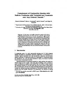
Figure 2: The decision tree for the tall query Q.
4.3
Tall Queries
We describe here the algorithm for the tall query Q(x, y, z) : −R(x), S(x, y), T (x, y, z). The generalization to arbitrary tall queries is straightforward and omitted. For the broadcast phase, we first set the thresholds τS = s/P log P and τT = t/P log P . Using any algorithm in Subsection 4.1, we compute the following sets: • SF 1 ⊇ {x | fS (x) ≥ τS } • T F 1 ⊇ {x | fT (x) ≥ τT } • T F 2 ⊇ {x, y | fT (x, y) ≥ τT } Next, each server constructs the decision tree of Figure 2. Consider a server s and any tuple t belonging to one of its fragments Rs , Ss , Ts . Depending on which of the relations t belongs to, a subset of the variables x, y, z is bound. That is, if t ∈ R then it binds x; if t ∈ S then it binds x, y; and if t ∈ T then it binds x, y, z. Starting from the root, we follow the decision tree until one of two things happens: • We reach a node asking for a variable not bound by t, e.g. if t ∈ R and we reach a node asking for x, y. In this case, we broadcast t to all the servers. • We reach a leaf of the tree. Then, we hash t according to the hash function with parameters the variables of the leaf node, that is, we send t either to h1(x) or to h2(x, y) or to h3(x, y, z). For example, consider a tuple S(a, b), such that a is frequent in T and a, b is not frequent in T . Then, this tuple will be sent to server h2(a, b). After distributing the tuples, each server locally computes the join. Theorem 4.4. For |S|, |T | large enough: |S|/ log |S| = Ω(P 2 log P ) (similarly for T ), the algorithm for computing the tall query Q is load balanced and has one MP step. Proof. First, consider all the tuples that are broadcast by the algorithm. R may broadcast at most P log P tuples for frequent values in S and T . Moreover, S may broadcast a tuple for a frequent value in T , which are at most P log P . Hence, each server receives at most 3 · P log P = O(n/P ) such tuples, since n = Ω(P 2 log P ). Thus, it suffices to measure the load caused by the tuples which are hashed. We partition the tuples into equivalence classes (balls), according to the values they are hashed on (notice that it suffices to consider only input tuples, since the output size is at most the input size). For example, ball B(a) contains all tuples from R, S, T which are hashed only to h1(a). Notice also that if a ∈ T F 1 , then B(a) is empty. The following properties hold for any ball: 1. 2. 3. 4.
Every tuple of a ball is sent to the same server. Every ball is sent to a u.a.r. chosen server. The maximum size wmax of a ball is (s + t)/(P log P ). The total size of the balls is W ≤ |R| + |S| + |T |.
We only prove property (3), since the others are straightforward. Consider the case for a ball B(a). Any tuple from S belonging to B(a) is hashed only on the x variable; hence, by the structure of the decision tree, a ∈ SF 1 , which implies that fS (a) < τS ; hence, there exist at most τS such tuples. Similarly, we have at most τT tuples from T in B(a). Thus, |B(a)| < 1 + τS + τT . For a B(a, b) ball, we have that |B(a, b)| < 2 + τT (and for B(a, b, c) the size is constant). Following from these properties, the expected maximum load is maximized in the case of W/wmax balls with size wmax . Using the same argument as in the proof of Theorem 4.1, | ). we obtain that E[maxs ns ] = Θ( |R|+|S|+|T P
5. THE MAIN ALGORITHM In this section, we show how the techniques presented in the previous sections can be combined to build a load balanced algorithm for any tall-flat query. For ease of exposition, let us denote by x1:k the sequence of variables or values x1 , x2 , . . . , xk . We will also assume w.l.o.g. the following form for tall-flat queries: Q(x1:k , y1:ℓ ) = R1 (x1 ), . . . , Rk (x1:k ), S1 (x1:k , y1 ), . . . , Sℓ (x1:k , yℓ ). For simplicity, we will also refer to S1 , . . . , Sℓ as Rk+1 , . . . , Rk+ℓ . For the algorithm, we will assume that Ri , Si are large enough: in particular, we will need that |Ri |/ log |Ri | = Ω(P 2 log P ) and that |Si |/ logℓ |Si | = Ω(P l+1 log P ). We also define p the frequency thresholds τRi = |Ri |/P log P and τSi = ℓ |Si |/P log P . In order to distribute the tuples in a load balanced way, the algorithm considers two cases: (1) values which cause a large load to the query result Q and (2) the rest of the values. Intuitively, we use flat-query techniques to deal with the first case and tall-query techniques for the second case. Broadcast Phase Broadcast 1: Using any of the algorithms in Subsection 4.1, compute the sets RFij ⊇ {x1:j | fRi (x1:j ) ≥ τRi } (i = 1, k; j = 1, i) SFij ⊇ {x1:j | fSi (x1:j ) ≥ τSi } (i = 1, ℓ; j = 1, k) In particular, using Frequency Sampling, we can compute these sets by sampling only once. One can easily check that the communication is O(nε ). Broadcast 2: For every relation V 6= Si , server s computes SFi (V, s) = SFik ∩Vs , i.e. intersects SFik with its local copy of V . These sets are then broadcast. `SFinally, each ´ T server computes the sets SFi = V 6=Si s SFi (V, s) . Communication Phase S
1. For i = 1, . . . , ℓ: for every x1:k ∈ SFi \ j q, in which case we broadcast x1:q , or when i = 0 (a leaf is reached) and the tuple is hashed to h(x1:j ). Computation Phase The query is locally computed at each server.
Theorem 5.1. The algorithm computes any tall-flat query in a load balanced way and has one MP step. Proof. We first analyze the load for the tuples that fall into the first case of the communication phase. Let us consider the case of the FOR loop where i = 1 (the same argument can be applied for every i). Consider a value x1:k ∈ SFQ The total load 1. P attributed to this value is N (x1:k ) = ℓi=1 fSi (x1:k ) + i=1,ℓ fSi (x1:k ). Since any tuple from S1 containing x1:k is hashed on (x1:k , y1 ), using the balls in bins argument, we have E[maxs Ns (x1:k )] ≤ P Qℓ i>1 fSi (x1:k )+(2fS1 (x1:k )/P )·(1+ i=2 fSi (x1:k )). Moreover, notice that fSi (x1:k ) ≥ 1 is guaranteed from the second step of the broadcast phase and also fS1 (x1:k ) ≥ P . Thus, E[max Ns (x1:k )] ≤ s
ℓ 2k Y · fS (x1:k ) P i=1 i
We next consider the values of the second case. In order to compute the load from the tuples that are broadcast to all servers, notice that we have O(P log P ) frequent values for each x1:j in relation Ri , hence a total load of O(k2 P log P ) for each server. As for relations Si , we have |Si |/τSi frequent values for each x1:j in Si . Thus, each relation causes a load of O(k ·|Si |/τSi ) to each server from broadcasting tuples. As long as |Si | ≥ P ℓ+1 log P , this load is bounded by O(|Si |/P ). Finally, let us also measure the load caused by the tuples which are hashed. We partition the tuples into equivalence classes (balls), according to the values they are hashed with. Notice that every ball has the following properties: (1) every tuple of a ball is sent to exactly one server, and (2) every ball is sent to a u.a.r. chosen server. Now, consider a ball B(x1:q ), q ≤ k. We define the size of the ball to include the size of the output. Consider any tuple t from a relation Ri belonging to B(x1:q ). Clearly, for i ≤ q, each relation Ri sends at most one tuple to this ball. For Ri , i > q, by the structure of the decision tree, fRi (x1:q ) < τRi and thus there exist at most τRi such tuples. The same holds for any Si . Thus, |B(x1:q )| ≤ q +
k X
τRi +
i=q+1
ℓ X i=1
τSi + |QB(x1:q ) |
where QB(x1 ) denotes the tuples of Q produced by the tuples in B(x1:q ). Next, notice that |QB(x1:q ) | =
X
ℓ Y
fSi (x1:q , xq+1:k )
xq+1:k ∈B(x1:q ) i=1
Since every tuple is hashed only on x1:q , it must hold that P xq+1:k ∈B(x1:q ) fSi (x1:q , xq+1:k ) ≤ τSi . This implies that |QB(x1:q ) | is maximized when there exists a value x′q+1:k such that for every Si , fSi (x1:q , x′q+1:k ) = τSi (and zero for all the other values). Then, using the Arithmetic-Geometric means inequality, we obtain that Pℓ Qℓ ℓ 1/ℓ Y si s 1 |QB(x1:q ) | ≤ τSi = i=1 i ≤ · i=1 P log P ℓ P log P i=1 , (c is some constant); This implies that |B(x1:q )| ≤ c· size(D) P log P
hence wmax = c · size(D) . P log P Let W be the total load of the balls. The expected maximum load is maximized when we have just W/wmax balls with size wmax . Using the same argument as in the proof of Theorem 4.1, we obtain that the expected maximum weight attributed to the hashed values is Θ(W/P ). Summing over all cases, we conclude that the algorithm is indeed load balanced.
6. IMPOSSIBILITY RESULTS In this section we prove that any query that is not tall-flat cannot be computed in one MP step. First, we show this result for two specific queries, RST (x, y) : −R(x), S(x, y), T (y) and J(x, y) : −R(x), S(x), T (y). Using these results, we prove the claim for any query that is not tall-flat. Theorem 6.1. Any algorithm that computes the query RST (x, y) : −R(x), S(x, y), T (y) in one MP step is skewed. Proof. Let A be a one step, load balanced algorithm for RST . Recall from the proof of Proposition 3.5 that we assume that R, S, T are partitioned separately. Using Corollary 3.8, we construct vectors X = (x1 , . . . , xn ) and Y = (y1 , . . . , yn ), such that we can substitute each value xi (yi ) with a value x′i (yi′ ) and obtain a colluding set. Now, let us consider an instance D of the database where R = X, T = Y and S = {(xi , yi ) | i = 1, . . . , n}. Fix also a run h ∈ H such that the computation for this instance is load balanced. Let us first consider the broadcast phase. Since R, T contain disjoint elements and the information exchanged may be only generic (i.e. obtained by generic computations on the instance), the only way for the servers to gain any information about the other relations is to exchange tuples R(xi ), or T (yi ), or S(xi , yi ): we say that the values xi ∈ X or yi ∈ Y or both have been broadcast. The total amount of communication is bounded by O(nε ), hence at most O(nε ) values from X and from Y are broadcast. Let X ′ and Y ′ be the other values, that are not broadcast: hence |X ′ | = n−O(nε ) and similarly for |Y ′ |. Let S ′ = {(xi , yi ) | xi ∈ X ′ , yi ∈ Y ′ }; it follows that |S ′ | = n − O(nε ). Claim: Suppose that we replace S by Sπ such that Sπ = {(xi , yi ) | (xi , yi ) ∈ / S ′ } ∪ {(xi , yπ(i) ) | (xi , yi ) ∈ S ′ }, where π is any permutation on the indices of S ′ . Let us call this instance Dπ . Using the argument in Corollary 3.8, we can prove that every server containing R, T tuples will receive exactly the same information under D or Dπ . Thus, the tuples of R, T will be distributed as before, that is, in a load balanced way. Denote R′ = X ′ and T ′ = Y ′ . We say that a pair (R′ (xi ), T ′ (yj )) meets when both tuples are placed in the same server. We next compute the total number of pairs which meet for an instance Dπ . Since each server holds O(n/P ) tuples from R′ , T ′ , it contains at most O(n2 /P 2 ) pairs that meet, which gives us a total of O(n2 /P ) pairs. However, drawing values from R′ , T ′ , there are O(n2 ) possible pairs. By the pigeonhole principle, there exists a pair such that R(xi ), T (yj ) are not placed in the same server. Then, we fix a permutation π such that the tuple S(xi , yj ) appears in Sπ . Finally, let us examine the instance Dπ : R, T, Sπ . For this instance, the tuple (xi , yj ) is included in the final result. However, the server s where S(xi , yj ) is sent can not contain both R(xi ), T (yj ). Let us assume w.l.o.g. that it does not contain R(xi ). Then, consider the instance Dπ′ where we substitute the tuple R(xi ) with R(x′i ). Following from the collusion property, and since x′i or xi are not communicated during the broadcast phase, the computation will be identical. This time, however, the tuple (xi , yj ) does not belong in the output. Nevertheless, the server s that decides upon whether to output the tuple or not does not contain x′i ; due to the genericity of the computation, s must again output the tuple (xi , yj ), which leads to a contradiction. Theorem 6.2. Any algorithm that computes the query J(x, y) : −R(x), S(x), T (y) in one MP step is skewed.
Proof. Let A be an algorithm computing J. First, we fix the instance of T = {y1 , . . . , yn }. Applying Corollary 3.8, we can then find a vector X = (x1 , . . . , xn ) with distinct elements, such that for each element xi ∈ X, there exists a vector Xi′ where xi is replaced by x′i 6= xi and X, Xi′ collude. Now, let us consider an instance D of the database where R = X and S = {x′i | xi ∈ X}. Following our construction, R and S are disjoint. P This means that J is empty and thus the total load is s ns = O(n). Since A is load balanced, there exists a run h ∈ H such that the computation is load balanced. Notice that, since the elements are disjoint within each relation and we allow only generic computation during the broadcast phase, the only way to gain information is by sending tuples. However, the amount of tuples we can send is limited to O(nε ). This means that from each relation, at most O(nε ) tuples can be sent to other servers. From this point, we consider only the tuples t ∈ R, such that t, t′ are not communicated (call these set R′ ). Clearly, |R′ | = n − O(nε ). We similarly define S ′ . We say that a pair of elements (xi , yj ) meets when T (yj ) is placed in the same server with either R′ (xi ) or S ′ (x′i ). Since each server receives at most O(n/P ) values from each relation, each server holds O(n2 /P 2 ) pairs that meet; in total, O(n2 /P ) pairs. However, the total number of possible pairs is O(n2 ). This implies that, by the pigeonhole principle, we can find a pair (xi , yj ) such that the tuple T (yj ) does not occur in the same server with either R(xi ) or S(x′i ). For the last step of the proof, consider an instance D′ where we replace in R the value xi with x′i . The servers will receive exactly the same information, since xi or x′i are not communicated during the broadcast phase. Thus, due to the collusion property, the behavior of the algorithm will be identical and, for the new instance, T (yj ) will not be placed in the same server as R(x′i ), S(x′i ). Consequently, A will not include the tuple (x′i , yj ) in the query output, which is a contradiction, sine (x′i , yj ) now belongs in the final result. Based on Theorem 6.1 and Theorem 6.2, we can now prove the following characterization. Theorem 6.3. Let Q be any query that is not tall-flat. Any algorithm that computes Q in one M P step is skewed. Proof. We first show that the queries computable in one MP step are a subset of hierarchical queries. Indeed, consider a query Q which is not hierarchical. Then, there exists a pair of variables x, y such that at(x)∩at(y) 6= ∅ and none of at(x), at(y) is a subset of the other. This means that w.l.o.g. we can find atoms R, S, T such that at(x) \ at(y) = {R}, at(y) \ at(x) = {T } and at(x) ∩ at(y) = {S}. Fix any variable 6= x, y to obtain the same constant value in any relation. Then, Q reduces to computing the query RST (x, y) : −R(x), S(x, y), T (y), which by Theorem 6.1 cannot be computed in one MP step. We also have the following property: if |at(x)| > 1 for a variable x, then for every variable y we have that at(x) ∩ at(y) 6= ∅. Indeed, if that was not true, then by fixing all other variables 6= x, y to obtain the same constant value, we reduce Q to J(x, y) : −R(x), S(x), T (y), which cannot be computed in one MP step by Theorem 6.2. Thus, if x appears in more than one relation, then for every variable y 6= x it holds that either at(x) ⊆ at(y) or at(y) ⊆ at(x). Let us now order the m variables in decreasing order of |at(x)|: x1 , x2 , . . . , xm . Consider the smallest index k such that for every i > k, |at(xi )| = 1. Using the above property,
for the first k variables we have that at(x1 ) ⊇ at(x2 ) . . . ⊇ at(xk ). Finally, consider a variable xj , j > k; by construction |at(xj )| = 1. We use again the property to see that for any i ≤ k, at(xj ) ⊆ at(xi ), since at(xj ) is a singleton set. Thus, Q satisfies all three properties of a tall-flat query.
7. DISCUSSION Star queries. Consider the following question: given a query Q, what is the smallest number of MP steps necessary to compute Q ? We answer this question for star queries, and leave it open for arbitrary conjunctive queries. W.l.o.g. we assume that the star query is of the form Q(x1 , . . . , xk ) : −R(x1 , . . . , xk ), S1 (x1 ), . . . , Sk (xk ). Since Q is not tall-flat, we need at least two MP steps to compute it. We show here that two steps are indeed optimal. Proposition 7.1. A star query can be computed in two M P steps. Proof. The load balanced algorithm for any star query works as follows. In the first step, compute all subqueies Qi (x1 , . . . , xk ) : −R(x1 , . . . , xk ), Si (xi ) in parallel, in one MP step (each is a semijoin query). In the second step, compute the intersection Q(¯ x) : −Q1 (¯ x), Q2 (¯ x), . . . , Qk (¯ x) (this MP step does not need a broadcast phase). General queries. If Q is a general conjunctive query, it seems difficult to determine the minimum number of parallel steps required to compute Q, because the intermediate results may be much larger than the output. For example, the output may be empty, but in any query plan, some subplan may return an intermediate result whose size is quadratic in the size of the input. One possibility is to adjust the definition of load balance to include in n the size of any intermediate computations. An algorithm for this case would work as follows. Let us assume a query Q and a query plan P for Q. First, reduce the nodes of P by combining consecutive query computations which correspond to a tall-flat query in one MP step. For example, if the plan operator computes P1 (x) : −R(x), S(x) and its parent computes P2 (x) : −P1 (x), T (x), then we compress the computation in one step: P2 (x) : −R(x), S(x), T (x), since it is a flat query. Each plan P can be thus converted into a minimal plan P ′ ; let d be its depth. It is easy to observe that one can compute P ′ in d MP steps. Example 7.2. Let us consider the following chain query: C(x, y, z, w, v) : −R(x, y), S(y, z), T (z, w), U (w, v). A naive query plan would sequentially compute the 3 joins to get the final result: this requires 3 M P steps. However, we can do better if we consider the following query plan: (R(x, y) ✶ S(y, z)) ✶ (T (z, w) ✶ U (w, v)) This plan corresponds to a query tree of depth 2; notice that R ✶ S and T ✶ U can be computed in parallel in the same M P step. Hence, we can compute the query in just two M P steps, which is also optimal (since it is not tall-flat). This example generalizes to any chain query: a chain query with k atoms can be computed in log k MP steps. Using Data Statistics. So far, our discussion has focused on the worst case scenario, and both our algorithms and our impossibility results assumed that the sizes of the input relations are independent. In practice, one often knows the sizes of the relations, and can determine that one is much larger than the other. Afrati and Ullman [1] have shown how to compute any conjunctive query in one parallel step. We illustrate their algorithm on the k-way star
query Q at the beginning of this section. Assume that the P processors are organized in a k-dimensional grid. Thus, each server √ is indexed by a k-tuple of integers (s1 , . . . , sk ), where k P ], for i = 1, k. For each i = 1, k, let hi : U → s√ i ∈ [ k [ P ] be a hash function. Then, during the communication phase the algorithm sends R(x1 , . . . , xk ) to the server (h1 (x1 ), . . . , hk (xk )) and replicates Si (xi ) to all servers of the form (∗, ∗, . . . , hi (xi ), . . . , ∗); in other words, Si (xi ) is √ k replicated P k−1 times. In the computation phase, each server computes the join locally. Thus, the algorithm takes a single communication step. In our framework, the algorithm is skewed, because it replicates the relations Si . However, suppose that it holds |R| = n, |S1 | = . . . = |Sk | = m, and √ k m P k−1 = O(n); then the algorithm is load balanced, and computes the star query in one step. This discussion shows that better MP algorithms can be designed by taking into account statistics on the input relations.
8.
CONCLUSIONS
In this work, we propose a new theoretical model which captures massive parallelism in today’s systems. In this model, the measure of complexity consists of the number of parallel steps necessary to compute a query. Under this context, we study the complexity of conjunctive queries and we give a complete characterization of the queries computable in one parallel step. Future work may include several directions: for any given conjunctive query, can we find the most efficient query plan in terms of steps of the MP model; what is the parallel complexity for more general sets of queries (e.g. queries with unions); and, finally, how can we implement and make the algorithms presented here practical. Acknowledgments. We would like to thank Foto Afrati, Magda Balazinska, Bill Howe, YongChul Kwon and Jeffrey Ullman for the useful discussions and suggestions.
9.
REFERENCES
[1] F. N. Afrati and J. D. Ullman. Optimizing joins in a map-reduce environment. In EDBT, pages 99–110, 2010. [2] P. Alvaro, W. Marczak, N. Conway, J. M. Hellerstein, D. Maier, and R. C. Sears. Dedalus: Datalog in time and space. Technical Report UCB/EECS-2009-173, EECS Department, University of California, Berkeley, Dec 2009. [3] L. Carter and M. N. Wegman. Universal classes of hash functions. J. Comput. Syst. Sci., 18(2):143–154, 1979. [4] R. Chaiken, B. Jenkins, P.-A. Larson, B. Ramsey, D. Shakib, S. Weaver, and J. Zhou. Scope: easy and efficient parallel processing of massive data sets. Proc. VLDB Endow., 1:1265–1276, August 2008. [5] S. Cohen. Containment of aggregate queries. SIGMOD Record, 34(1):77–85, 2005. [6] D. E. Culler, R. M. Karp, D. A. Patterson, A. Sahay, K. E. Schauser, E. E. Santos, R. Subramonian, and T. von Eicken. Logp: Towards a realistic model of parallel computation. In PPOPP, pages 1–12, 1993. [7] N. N. Dalvi and D. Suciu. Efficient query evaluation on probabilistic databases. VLDB J., 16(4):523–544, 2007. [8] J. Dean and S. Ghemawat. Mapreduce: Simplified data processing on large clusters. In OSDI, pages 137–150, 2004. [9] D. J. DeWitt and J. Gray. Parallel database systems: The future of high performance database systems. Commun. ACM, 35(6):85–98, 1992. [10] A. Gates, O. Natkovich, S. Chopra, P. Kamath, S. Narayanam, C. Olston, B. Reed, S. Srinivasan, and U. Srivastava. Building a highlevel dataflow system on top of mapreduce: The pig experience. PVLDB, 2(2):1414–1425, 2009. [11] M. Grohe, Y. Gurevich, D. Leinders, N. Schweikardt, J. Tyszkiewicz, and J. V. den Bussche. Database query processing using finite cursor machines. Theory Comput. Syst., 44(4):533–560, 2009. [12] J. M. Hellerstein. The declarative imperative: experiences and conjectures in distributed logic. SIGMOD Rec., 39:5–19, September 2010.
[13] N. Immerman. Expressibility and parallel complexity. SIAM J. Comput., 18(3):625–638, 1989. [14] H. J. Karloff, S. Suri, and S. Vassilvitskii. A model of computation for mapreduce. In SODA, pages 938–948, 2010. [15] P. Koutris and D. Suciu. Parallel evaluation of conjunctive queries. Research Report UW-CSE-11-03-01, University of Washington, 2011. [16] L. Libkin. Elements of Finite Model Theory. Springer, 2004. [17] S. Melnik, A. Gubarev, J. J. Long, G. Romer, S. Shivakumar, M. Tolton, and T. Vassilakis. Dremel: Interactive analysis of web-scale datasets. PVLDB, 3(1):330–339, 2010. [18] A. Pagh and R. Pagh. Uniform hashing in constant time and optimal space. SIAM J. Comput., 38(1):85–96, 2008. [19] M. Raab and A. Steger. ”balls into bins” - a simple and tight analysis. In RANDOM, pages 159–170, 1998. [20] P. Sanders. On the competitive analysis of randomized static load balancing. In Proceedings of the first Workshop on Randomized Parallel Algorithms, RANDOM, 1996. [21] L. J. Stockmeyer and U. Vishkin. Simulation of parallel random access machines by circuits. SIAM J. Comput., 13(2):409–422, 1984. [22] A. Thusoo, J. S. Sarma, N. Jain, Z. Shao, P. Chakka, S. Anthony, H. Liu, P. Wyckoff, and R. Murthy. Hive - a warehousing solution over a map-reduce framework. PVLDB, 2(2):1626–1629, 2009. [23] L. G. Valiant. A bridging model for parallel computation. Commun. ACM, 33(8):103–111, 1990. [24] Y. Xu, P. Kostamaa, X. Zhou, and L. Chen. Handling data skew in parallel joins in shared-nothing systems. In SIGMOD ’08: Proceedings of the 2008 ACM SIGMOD international conference on Management of data, pages 1043–1052, New York, NY, USA, 2008. ACM. ´ Erlingsson, P. K. [25] Y. Yu, M. Isard, D. Fetterly, M. Budiu, U. Gunda, and J. Currey. Dryadlinq: A system for general-purpose distributed data-parallel computing using a high-level language. In OSDI, pages 1–14, 2008.
APPENDIX Proposition A.1. Frequency Sampling ( Subsection 4.1) includes in F every value x with fR (x) ≥ τ with high probability. Moreover, for some constant b, F contains no value x′ with fR (x′ ) < b · τ w.h.p. Proof. The proof is based on a standard application of Chernoff bounds. For the first part, we compute the probability that a frequent value a is not included in F . The probability that we sample a tuple with this value is fR (a)/r ≥ τ /r and the probability that a ∈ / F equals the probability that tuples with a are sampled less than c·τ ·T /r times. If K(a, v), we denote v by f ′ (a), i.e. f ′ (a) gives the estimation for the frequency of a. Then, P r[a ∈ / F] = P r[f ′ (a) < c · τ · T /r]. Notice that each sample is an independent random choice ′ and P a is chosen with probability ≥ τ /r. Moreover, E[f (a)] = f (a)/r ≥ τ · T /r. We can thus apply the Chernoff j=1,T R bound with δ = (c − 1)/c, which gives us that P r[f ′ (a) < ′ 2 c·τ ·T ] ≤ P r[f ′ (a) < (1 − δ) · E[f ′ (a)]] < e−E[f (a)]δ /2 . Since r there are ≤ r/τ frequent values, we can apply a union bound: P ′ 2 P r[∃a ∈ / F ] ≤ a:fR (a)≥τ P r[a ∈ / F ] < (r/τ )e−E[f (x)]δ /2 = r , (r/τ )e−C·τ ·T /r , where C = (c − 1)2 /2c2 . For T = d1 · r log τ where d1 is a constant, the probability of failure becomes arbitrarily small. For the second part, consider a value a such that fR (a) < b · τ for some constant b < 1. Using similar arguments as above, we can show that E[f ′ (a)] < b · τ · T /r. We apply again the Chernoff bound (for a suitable choice of δ): P r[a ∈ F ] = P r[f ′ (a) ≥ c·τr·T ] = P r[f ′ (a) > (1 + δ) · E[f ′ (a)]] < ′ 2−(1+δ)·E[f (a)] = 2−C·τ ·T /r , where C is some constant depending on b, c. We use again a union bound to get that P ·T − C·τ r . For P r[∃a ∈ F ] ≤ a:fR (a)