We introduce the graph coloring problem, a classical problem in graph theory, using this ... of multiprocessor parallel computers for achieving increased computational speed. ...... presentation of coloring algorithms throughout this thesis. The graph ...... [19] Vipin Kumar, Ananth Grama, Anshul Gupta, and George Karypis. In-.
Parallel Graph Coloring By Assefaw Hadish Gebremedhin Thesis submitted in partial fulfilment of the requirements for the degree of
Candidatus Scientiarum
Department of Informatics University of Bergen Norway
Spring 1999
2
i
Acknowledgements My deepest gratitude goes to my advisor, Associate Professor Fredrik Manne, for his guidance, support, motivation and encouragement throughout the period this work was carried out. His readiness for consultation at all times, his educative comments, his concern and assistance even with practical things have been invaluable. A vote of thanks to fellow students and the staff at the Department of Informatics for their friendly co-operation and all Ethiopian students at the University of Bergen, in particular Zewdie Haileselassie, for their friendship and the memorable social gatherings. I am grateful to my parents, Hadish Gebremedhin and Alganesh Tsegay, my sister Menen, Aman and all my brothers for their moral support and encouragement. Finally, I direct special thanks to a special friend, Dr. Tsigeweini Asgedom. Tsigina, thank you for your love, support, encouragement and not least for proof-reading this thesis. Bergen, April 14, 1999 Assefaw Hadish Gebremedhin
Contents 1 Introduction
1
1.1
Graph Theoretic Definitions and Notations . . . . . . . . . .
6
1.2
Problem Definition . . . . . . . . . . . . . . . . . . . . . . . .
6
1.3
NP-complete Problems . . . . . . . . . . . . . . . . . . . . . .
7
2 Coping with NP-Completeness
10
2.1
Special Cases . . . . . . . . . . . . . . . . . . . . . . . . . . .
10
2.2
Backtracking and Branch-and-Bound . . . . . . . . . . . . . .
11
2.3
Heuristics . . . . . . . . . . . . . . . . . . . . . . . . . . . . .
11
2.3.1
Categories of Heuristics . . . . . . . . . . . . . . . . .
12
2.3.2
Measuring Performance of Heuristics . . . . . . . . . .
13
2.4
2.5 2.6
Approximation Algorithms
. . . . . . . . . . . . . . . . . . .
13
2.4.1
Definition of Approximation Algorithm . . . . . . . .
13
2.4.2
Approximation Schemes . . . . . . . . . . . . . . . . .
14
2.4.3
Inapproximability
. . . . . . . . . . . . . . . . . . . .
14
Randomized Algorithms . . . . . . . . . . . . . . . . . . . . .
15
2.5.1
Measuring Performance of Randomized Algorithms . .
15
Other Methods . . . . . . . . . . . . . . . . . . . . . . . . . .
15
3 Multiprocessor Parallel Processing
17
3.1
Why Parallel Processing? . . . . . . . . . . . . . . . . . . . .
17
3.2
Theoretical Considerations . . . . . . . . . . . . . . . . . . . .
18
3.2.1
Parallel Machine Model . . . . . . . . . . . . . . . . .
18
3.2.2
Parallel Complexity . . . . . . . . . . . . . . . . . . .
20
ii
iii
CONTENTS
3.2.3 3.3
Basic Parallelization Techniques . . . . . . . . . . . .
20
Practical Considerations . . . . . . . . . . . . . . . . . . . . .
20
3.3.1
Parallel Programming Models . . . . . . . . . . . . . .
21
3.3.2
Performance Metrics for Parallel Systems . . . . . . .
22
4 Review of Graph Coloring Heuristics
24
4.1
Theoretical Results . . . . . . . . . . . . . . . . . . . . . . . .
24
4.2
Sequential Graph Coloring Heuristics . . . . . . . . . . . . . .
25
4.2.1
Greedy Coloring Heuristics . . . . . . . . . . . . . . .
25
4.2.2
Local Improvement Coloring Heuristics . . . . . . . .
32
Parallel Graph Coloring Heuristics . . . . . . . . . . . . . . .
34
4.3.1
Parallel Maximal Independent Set (MIS)
. . . . . . .
35
4.3.2
Jones-Plassmann . . . . . . . . . . . . . . . . . . . . .
35
4.3.3
Largest Degree First (LDF) . . . . . . . . . . . . . . .
38
4.3
5 New Parallel Graph Coloring Heuristics
39
5.1
Introduction . . . . . . . . . . . . . . . . . . . . . . . . . . . .
39
5.2
Graph Partitioning Approach . . . . . . . . . . . . . . . . . .
41
5.2.1
Definitions and Notations . . . . . . . . . . . . . . . .
41
5.2.2
The Algorithm . . . . . . . . . . . . . . . . . . . . . .
42
Block Partitioning Approach . . . . . . . . . . . . . . . . . .
44
5.3.1
The Algorithm . . . . . . . . . . . . . . . . . . . . . .
46
5.3.2
Results . . . . . . . . . . . . . . . . . . . . . . . . . .
46
Improved, Block Partition Based Coloring . . . . . . . . . . .
49
5.4.1
The Algorithm . . . . . . . . . . . . . . . . . . . . . .
49
5.4.2
Results . . . . . . . . . . . . . . . . . . . . . . . . . .
51
Hybrid . . . . . . . . . . . . . . . . . . . . . . . . . . . . . . .
52
5.3
5.4
5.5
6 Implementation
54
6.1
Graph Representation and Storage . . . . . . . . . . . . . . .
54
6.2
Determination of Smallest Legal Color . . . . . . . . . . . . .
55
6.3
Graph Partitioning Program . . . . . . . . . . . . . . . . . . .
56
iv
CONTENTS
6.4
OpenMP . . . . . . . . . . . . . . . . . . . . . . . . . . . . . .
56
6.5
Origin 2000 . . . . . . . . . . . . . . . . . . . . . . . . . . . .
58
6.6
Data Distribution . . . . . . . . . . . . . . . . . . . . . . . . .
58
7 Experimental Results and Discussion
62
7.1
Test Graphs . . . . . . . . . . . . . . . . . . . . . . . . . . . .
63
7.2
Results and Discussion . . . . . . . . . . . . . . . . . . . . . .
63
7.2.1
Graph Partitioning . . . . . . . . . . . . . . . . . . . .
64
7.2.2
Block Partitioning . . . . . . . . . . . . . . . . . . . .
65
7.3
Summary . . . . . . . . . . . . . . . . . . . . . . . . . . . . .
69
7.4
Further Research . . . . . . . . . . . . . . . . . . . . . . . . .
70
List of Figures 4.1
First Fit Coloring Algorithm . . . . . . . . . . . . . . . . . .
26
4.2
General Greedy Coloring Scheme . . . . . . . . . . . . . . . .
27
4.3
Coloring by removing independent sets . . . . . . . . . . . . .
30
4.4
Greedy Independent Set . . . . . . . . . . . . . . . . . . . . .
31
4.5
A Parallel Coloring Heuristic . . . . . . . . . . . . . . . . . .
34
4.6
Luby’s Monte Carlo algorithm for determining a MIS . . . . .
36
4.7
High-level, Jones-Plassmann coloring algorithm . . . . . . . .
37
5.1
Graph Partition Based Coloring Scheme . . . . . . . . . . . .
43
5.2
Block Partition Based Coloring Algorithm . . . . . . . . . . .
45
5.3
Improved, Block Partition Based Coloring Algorithm . . . . .
50
5.4
Hybrid Coloring Algorithm . . . . . . . . . . . . . . . . . . .
53
6.1
Data distribution . . . . . . . . . . . . . . . . . . . . . . . . .
60
6.2
An example of the use of data distribution . . . . . . . . . . .
60
7.1
Speedup comparison I . . . . . . . . . . . . . . . . . . . . . .
77
7.2
Speedup comparison II . . . . . . . . . . . . . . . . . . . . . .
78
7.3
Speedup comparison III . . . . . . . . . . . . . . . . . . . . .
79
v
List of Tables 7.1
Problem Set I . . . . . . . . . . . . . . . . . . . . . . . . . . .
62
7.2
Problem Set II . . . . . . . . . . . . . . . . . . . . . . . . . .
63
7.3
Problem Set III . . . . . . . . . . . . . . . . . . . . . . . . . .
63
7.4
Results of graph partition based coloring . . . . . . . . . . . .
72
7.5
Speedup using graph partition based coloring . . . . . . . . .
73
7.6
Results of simple block partition based coloring . . . . . . . .
74
7.7
Results of improved, block partition based coloring . . . . . .
75
7.8
Speedup using block partition based coloring . . . . . . . . .
76
vi
Chapter 1
Introduction Let us say you are asked to help out a cartographer or a map-maker with her map-coloring problem. She wants to color the countries on a map. It doesn’t matter which color a country is assigned, as long as its color is different from that of all bordering countries. If two countries meet only at a single point, they do not count as sharing a border and hence can be made the same color. The cartographer is poor and can’t afford many crayons, so the idea is to use as few colors as possible. In 1852 Francis Guthrie, while trying to color the map of countries of England, noticed that four colors sufficed. Subsequently, he conjectured that 4 colors are enough to color any map. Successive efforts made to prove Guthrie’s 4-color conjecture led to the development of much of graph theory. A graph is an abstract representation of relationships. Informally, it can be defined as a diagram consisting of points, called vertices, some of which are connected by lines, called edges. A vertex in a graph models some physical entity or abstract concept. An edge, which joins exactly two vertices, represents the relationship or association between the respective entities or concepts. The map of countries mentioned above can, for instance, be converted into an equivalent graph by letting each country be a vertex and connecting two vertices by an edge if the corresponding countries share a border, where sharing a border is as specified above. We introduce the graph coloring problem, a classical problem in graph theory, using this informal definition of graph. In its simplest form, the 1
2
CHAPTER 1. INTRODUCTION
graph coloring problem is to assign labels (called colors) to the vertices of a graph in such a way that no two vertices connected by an edge share the same label (color). The objective is to use the fewest number of colors possible. It is easy to observe that the map-coloring problem stated above can be modeled as a graph coloring problem. Such a graph, one which corresponds to some kind of map, is in fact called a planar graph. Today, it is a well known fact that 4 colors are enough to color any planar graph [15]. The graph coloring problem has a central role in computer science. It models many significant real-world problems, or arises as part of a solution for other important problems. The next few paragraphs highlight some of the major application areas. Time Tabling and Scheduling
Many scheduling problems involve al-
lowing for a number of pairwise restrictions on which jobs can be done simultaneously. For instance, in attempting to schedule classes at a university, two courses taught by the same instructor can not be scheduled for the same time slot. Similarly, two courses that are required by the same group of students should not be scheduled for the same time slot. The problem of determining the minimum number of time slots needed subject to these restrictions can be modeled by the graph coloring problem. Frequency Assignment
Another example is the problem of assigning
frequencies to mobile radios and other users of electromagnetic spectrum. In the simplest case, two customers that are sufficiently close must be assigned different frequencies, while those that are distant can share frequencies. The problem of minimizing the number of frequencies has been modeled [7] as a graph coloring problem. Register Allocation
One of the issues involved during program execution
is register allocation. The register allocation problem denotes the problem of assigning variables to a limited number of hardware registers. Variables
CHAPTER 1. INTRODUCTION
3
in registers can be accessed much quicker than those not in registers. Typically, however, there are far more variables than registers. This makes it necessary to assign multiple variables to registers. However, variables that are active in the same range of code cannot be placed in the same register. Such variables are said to conflict with each other. The goal of the register allocation problem is thus to assign non-conflicting variables to registers so as to minimize the use of variables not stored in registers. It has been shown that [4] this problem can be reduced to the graph coloring problem. Printed Circuit Testing
This is an example in which graph coloring is
used to speed up the testing of printed circuit boards for unintended short circuits caused by stray lines of solder [9]. Numerical Computation
Graph coloring arises as part of the solution
for many problems in computational science [1]. It has also reported applications in optimization [5] and parallel numerical methods [16]. Given its importance, one is interested in solving the graph coloring problem in a fastest and cost effective way possible. This goal is particularly important when one deals with graphs of very large size. The need for faster solutions and for solving larger-size problems arises in many other applications also. At present, technology has reached a stage where the fastest cycle time of a processor in a computer seems to be approaching fundamental physical limitations beyond which no improvement is possible. This, coupled with a steady decline in hardware cost, has led to the use of multiprocessor parallel computers for achieving increased computational speed. Currently, commercially available multiprocessor parallel computers are based on distributed-memory, shared-memory, or distributed-shared-memory architectures. The target computer of this study, the Cray Origin 2000, is an example of the last type. An on-line description of the architecture of the Origin 2000 installed at Parallab [26] states the following. “In effect, distributed-shared-memory architecture means that the memory is physi-
CHAPTER 1. INTRODUCTION
4
cally distributed and resides on the processors. However, for operational purposes, the system behaves as a shared memory computer with the operating system taking care of maintaining memory consistency. Thus any processor can use the total amount of memory.” The Cray Origin 2000 can be programmed both using shared memory and message passing programming (MPP) models. Generally MPP yields scalable applications but requires more programming incentive. The difficulty in MPP lies in the fact that it requires the program’s data structures to be explicitly partitioned. This means the entire application must be parallelized in order to work with the partitioned data structures. Moreover, in MPP, there is no incremental path to parallelizing an existing sequential application. Shared memory programming (SMP), on the other hand, does not require explicit partitioning of data structures and allows incremental parallelization of sequential applications. In general, however, SMP does not yield applications as scalable as MPP based applications. A portable, fork-join parallel model for SMP, called OpenMP has now emerged [25]. OpenMP supports two basic flavors of parallelism: coarsegrained and fine-grained. An OpenMP application program interface is available on our target computer. In spite of the general scalable performance of MPP based applications, existing parallel graph coloring algorithms are not scalable. The main reason for their usage so far has been the fact that they give access to more memory. The availability of distributed-shared memory architecture based parallel machines makes this argument not relevant any longer. This work is a study on how the graph coloring problem can be solved faster by decomposing it into several subproblems and solving the subproblems concurrently on a multiprocessor parallel computer. Specifically our task has been • to study existing parallel graph coloring algorithms, • to develop and analyze new parallel graph coloring algorithms, and
CHAPTER 1. INTRODUCTION
5
• to implement the new algorithms on Origin 2000 using SMP. Including this introductory chapter, this thesis consists of 7 chapters. The first three chapters present preliminary material required for the discussions in the main body of this thesis, Chapters 4 through 7. In the remaining sections of this chapter, we introduce the graph notations used in this thesis and give a brief introduction to the theory of NP-complete problems. In Chapter 2, different methods that can be used in dealing with NP-complete problems in general are discussed. Chapter 3 discusses briefly theoretical as well as practical matters regarding multiprocessor parallel computation in general. Chapter 4 is aimed at addressing our first task. It is a review of known sequential and parallel graph coloring algorithms. The chapter begins by a review of sequential coloring algorithms as they are the basis for the parallel ones. The sequential algorithms are classified into two categories: greedy and local improvement methods. These methods are introduced in Chapter 2. Chapter 5 deals with the second task. It presents the parallel coloring algorithms developed in this work. In this chapter, we present effective ways of decomposing the graph coloring problem into subproblems such that the subproblems can be solved concurrently. Analytical, performance analyses of the algorithms are provided. We also present a method of obtaining improved quality coloring using a two-phase coloring strategy. Chapter 6 relates to our third task. The chapter includes a discussion on the data structures used, a brief introduction to OpenMP, and a discussion on performance improvement using data distribution. Finally in Chapter 7 we present experimental results that demonstrate the performance of the algorithms presented in Chapter 5. The experimental results indicate that the algorithms behave as they are theoretically expected. We also provide some concluding remarks and point out possible directions for further research.
CHAPTER 1. INTRODUCTION
1.1
6
Graph Theoretic Definitions and Notations
A graph G is a pair (V, E) of a set of vertices V and a set of edges E. The edges are unordered pairs of the form (i, j) where i, j ∈ V . Two vertices i and j are said to be adjacent if and only if (i, j) ∈ E and non-adjacent otherwise. The degree of a vertex v is the number of vertices adjacent to v and is denoted by deg(v). The maximum, minimum, and average degree in a graph G are denoted by ∆, δ, and δ respectively. An induced subgraph of G = (V, E) is a graph G 0 = (V 0 , E 0 ) where V 0 ⊂ V and E 0 = {(i, j) such that (i, j) ∈ E, and i, j ∈ V 0 }. An independent set in a graph is a set of vertices that are mutually nonadjacent. This means that there is no edge between any pair of vertices in an independent set. A partition of a non-empty set A is a subset Π of 2 A such that 1. ∅ is not an element of Π and 2. each element of A is in one and only one set in Π. Given a graph G = (V, E) two vertices u and v are said to be connected if u = v or there exists a path P = (u = x1 , x2 , . . . , xk = v), such that (xi , xi+1 ) ∈ E , where 1 ≤ i ≤ k − 1. This relation is an equivalence 1 relation on V , and hence partitions V into equivalence classes V 1 , V2 , . . . , Vt . The subgraphs Gj = (Vj , Ej ), where Ej = {(x, y) ∈ E such that x, y ∈ Vj }, are called the connected components of G.
1.2
Problem Definition
In this section, we give a formal definition of the graph coloring problem and introduce two related problems that we encounter in our solution methods for the graph coloring problem. 1 A relation that is reflexive, symmetric, and transitive is called an equivalence relation
7
CHAPTER 1. INTRODUCTION
The graph coloring problem
A vertex coloring of a graph, or simply
coloring for short, is an assignment of colors to the vertices such that no two adjacent vertices are assigned the same color. Alternatively, a coloring is a partition of the vertex set into a collection of vertex-disjoint independent sets. Each independent set in such a partition is called a color class. The graph coloring problem is then to find a vertex coloring for a graph using the minimum number of colors possible. A k-coloring of a graph G is a coloring of G using k colors. The minimum possible value for k is called the chromatic number of G, denoted as χ(G). A coloring with the fewest possible number of colors (a χ-coloring) is called an optimal coloring. Related Problems
The independent set problem is to find an indepen-
dent vertex set of maximum cardinality. A simpler problem is finding a maximal independent set, an independent set that can not be extended further. The graph partitioning problem is to partition the vertices of a graph in p roughly equal parts such that the number of edges connecting vertices in different parts is minimized.
1.3
NP-complete Problems
In our context, a problem can be posed either in a decision or an optimization form. A decision problem is one that has a yes/no answer. If a decision problem asks about the existence of a structure with a certain value, then the corresponding problem of finding a structure with the best value is an optimization problem. For example, the graph coloring problem can be posed in its decision form as: given a graph G and an integer k, can the graph be k-colored? The corresponding optimization problem is: given a graph G, color the graph with the fewest number of colors possible. If the input of a decision problem is encoded as a string, the decision problem can alternatively be viewed as a language recognition problem where
CHAPTER 1. INTRODUCTION
8
the term language is defined as any set of strings over a given alphabet. Using this alternative view the graph coloring problem can be presented as a question of deciding membership in the language COLOR defined below. Let hG, ki denote the encoding of the inputs graph G and integer k as a string. COLOR ={hG, ki| G can be k-colored } The Turing machine (TM) is known to be a powerful computational model used for language recognition and computation of functions. We will not give a formal definition of the TM model here but instead use some general statements about it. A Turing Machine can either be deterministic or nondeterministic in its operation. According to the Church-Turing thesis [28], the TM model is equivalent to the concept of algorithm. Therefore an f (n)-time deterministic TM is another way of expressing an algorithm of time complexity f (n). A language is said to be decidable if some TM decides it. Languages (decision problems) are classified into different classes according to the time required to decide them. The class P consists of languages that are decidable in polynomial time on a deterministic TM. The class N P consists of languages that are decidable in polynomial time on a nondeterministic TM. The power of a nondetrminstic TM lies in its ability to “guess” the right branch in its computation tree that leads to a solution. The question of whether P = N P is one of the greatest unsolved problems in theoretical computer science and contemporary mathematics. Most researchers believe that the two classes are not equal. One important advance on the P versus NP question is the discovery of problems in NP whose individual complexity is related to that of the entire class. If a polynomial time algorithm exists for any one of these problems, all problems in NP would be polynomial time solvable. These problems are called NP-complete. A formal definition for an NP-complete problem requires us introduce the concept of polynomial time reducibility. Language A is polynomial time reducible to language B if a polynomial time computable function f exists,
CHAPTER 1. INTRODUCTION
9
where for every w , w ∈ A ⇐⇒ f (w) ∈ B. A language B is said to be NP-complete if it satisfies the following two conditions: 1. B is in NP, and 2. every A in NP is polynomial time reducible to B. A problem is called NP-hard if all problems in NP are polynomial time reducible to it, even though it may not be in NP itself. NP-completeness is only defined for decision problems. If a decision problem is NP-complete, then the corresponding optimization problem is NP-hard. The problem we are addressing in this thesis, the graph coloring problem, as well as the two related problems we have introduced, the independent set and graph partitioning problems, are all known to be NP-complete [8]. Moreover, the determination of the chromatic number of a graph is known to be NP-hard.
Chapter 2
Coping with NP-Completeness The graph coloring problem in its decision form is known to be NP-complete. This means that the problem has no polynomial time algorithm in sight and it is highly unlikely that it can have one. Nevertheless, stating this will not make the problem go away. What is there then to be done if one has to color a graph anyway? More generally, how does one solve NP-complete problems? In this chapter, we shall briefly discuss the most useful maneuvers employed in dealing with NP-completeness in general. One of the objectives of this chapter is to define the concepts that may be referred to later in this thesis.
2.1
Special Cases
Once a problem has been proved to be NP-complete, the first question to ask is the following. Do we really need to solve this problem in full generality in which it was formulated and proved NP-complete? Perhaps what we really need to solve is a more tractable special case of the problem. The graph coloring problem, for instance, renders trivial if the graph is restricted to be a tree. A tree is an undirected graph with no cycles. A coloring algorithm for a tree takes advantage of the hierarchical structure of trees. It is often useful in a tree to pick an arbitrary node and designate it as the root. Once this has been done, each node u in the tree becomes 10
CHAPTER 2. COPING WITH NP-COMPLETENESS
11
itself the root of a subtree T (u), the set of all nodes v such that the (unique) path from v to the root goes through u. Then the coloring problem can be solved by a top-down, level-by-level, traversal of the tree starting from the root. During this traversal, all the nodes in the same level on the tree are assigned the same color (one of two alternating colors). Thus the tree can be colored using only 2 colors in time proportional to the height of the tree.
2.2
Backtracking and Branch-and-Bound
After one makes sure that a special case is not what is desired to be solved or the special case is also NP-complete, then efforts are made to find a usable algorithm for handling the problem. One approach in this direction is the use of backtracking algorithms. Recall that all NP-complete problems are, by definition, solvable by polynomial time nondeterministic Turing machines. Unfortunately, we only know of exponential methods to simulate such machines. Backtracking algorithms try to improve on this exponential behavior with clever, problem-dependent strategies. They often do better than a straight forward exhaustive search. Backtracking algorithms are of interest when solving a decision problem. For optimization problems one often uses a variant of backtracking called branch-and-bound. Branch-and-bound algorithms require good lower and/or upper bounds of the optimum solution. The closer the bounds are to the optimum value the faster the branch-and-bound algorithm terminates. The need for good bounds makes branch-and-bound algorithms less attractive.
2.3
Heuristics
The other approach for solving NP-hard problems is the use of heuristics. A heuristic is usually a polynomial time algorithm that applies some rulesof-thumb to obtain an approximate solution to a problem. The goal of a heuristic is not to find an optimal solution but rather to find a good solution quickly.
CHAPTER 2. COPING WITH NP-COMPLETENESS
2.3.1
12
Categories of Heuristics
We distinguish between two categories of heuristics: greedy and local improvement. Greedy Heuristics A greedy heuristic makes the choice that seems best at the moment and proceeds until it finds a local optimum. Its name indicates that it is free of any backtracking. The main advantage of greedy heuristics is that they are fast (low-degree polynomial) and simple. Local Improvement Heuristics Local improvement heuristics are heuristics that iteratively try to improve the quality of a current solution for a problem. Two solutions are said to be neighbors if a simple operation results in a transition from one solution to the other. Such an operation could, for instance, be swapping a group of vertices between distinct color classes in the graph coloring problem. This successive transition from one solution to the other in search of an optimal solution is called neighborhood search. The quality of the solution obtained and the time required by a neighborhood search depend critically on the size of the neighborhood (search space) used initially. The larger the neighborhood the better the solution found but the longer the search takes. Local improvement heuristics are heuristics that seek a favorable compromise in this trade-off. Simulated annealing is one of the most widely used local improvement heuristics. Another well-known method, that may be characterized as a form of simulated annealing, is Tabu search. There exist several other related genres of local improvement methods, many of them based on some loose analogy with physical or biological systems. Examples include genetic algorithms and neural networks. Refer to Reeves [27] for a good coverage of modern heuristic methods.
CHAPTER 2. COPING WITH NP-COMPLETENESS
2.3.2
13
Measuring Performance of Heuristics
Often, the performance of a heuristic is judged by running it on a benchmark set of problem instances and comparing it with the performance of other heuristics on the same benchmark. This empirical approach is good for evaluating the comparative performance of heuristics within certain concrete application areas. However, the benchmark set, being typically a small sample, may not necessarily be a good representative of general problem instances. Thus improvements in the quality of a solution as measured by the benchmark set are not necessarily a good predictor of possible improvements in general cases. Another approach for measuring the performance of a heuristic is an average case analysis of its behavior. Such a result shows how the heuristic would “usually” behave. A disadvantage of such an analysis is that it assumes certain fixed distributions of the input. Average case analysis is, in general, complicated and only the simplest algorithms have been analyzed successfully.
2.4
Approximation Algorithms
The need for a well-defined analysis of the performance of heuristics led to the development of the formal concept of approximation algorithm. An approximation algorithm for an NP-hard problem is necessarily polynomial and the quality of its solution is measured by the worst case possible relative error over all possible instances of the problem. The error is measured against the optimal solution for the NP-hard problem. In the following sections, we shall define the central terms within the theory of approximation algorithms. The reason that we include these is to use the terms freely later in this thesis.
2.4.1
Definition of Approximation Algorithm
Formally, a polynomial algorithm A is said to be a δ-approximation algorithm if for every problem instance I with an optimal solution value OP T (I),
CHAPTER 2. COPING WITH NP-COMPLETENESS A(I) OP T (I)
14
≤ δ.
The ratio δ is referred to as the approximation ratio or performance guarantee. Obviously, δ > 1 for a minimization problem and δ < 1 for a maximization problem. The closer δ is to 1 the better.
2.4.2
Approximation Schemes
For some NP-hard problems, it is possible to invest more running time (still polynomial) in order to get a better approximation ratio. Schemes that reveal such a trade-off are called approximation schemes. There are two kinds of approximation schemes: polynomial and fully polynomial approximation schemes. Formally, a family of approximation algorithms for a problem P , {A � }� , is called a polynomial approximation scheme, if algorithm A � is a (1 + �)approximation algorithm and its running time is polynomial in the size of the input for a fixed �. The family is called a fully polynomial approximation scheme, if algorithm A� is a (1 + �)-approximation algorithm and its running time is polynomial in the size of the input and 1/�.
2.4.3
Inapproximability
All NP-hard problems are not equally difficult to approximate. The problems are divided into different classes based on the approximation ratio that is provably hard to achieve. These provably hard to achieve ratios are lower bounds1 beyond which the approximation can not be improved any further. Such results are called inapproximability results. Recent inapproximability results [13] divide NP-hard problems into classes I, II, III and IV. The corresponding hard to achieve approximation ratios are 1+� for some fixed � > 0, Ω(log n), 2log
1−γ
n
for every γ > 0, and nδ for some fixed δ > 0 respectively,
where n in all the cases is the input size. 1
The NP-hard problem is assumed to be a minimization problem
15
CHAPTER 2. COPING WITH NP-COMPLETENESS
2.5
Randomized Algorithms
Randomized algorithms as such are not means of solving NP-hard problems efficiently. However, once one has settled for an approximate solution for an NP-hard problem, randomized computation is an alternative computational paradigm to consider. A randomized algorithm is one that makes random choices during its execution. Randomized algorithms are interesting because, for many problems, they are considerably simpler or faster than the corresponding deterministic algorithms. There are two classes of randomized algorithms: Las Vegas and Monte Carlo. A randomized algorithm of the Las Vegas type always generates the correct answer, whereas the Monte Carlo type is allowed to make errors, but only with a “small” probability.
2.5.1
Measuring Performance of Randomized Algorithms
Since a randomized algorithm makes random choices during its execution, its resource requirement is measured in probabilistic terms. One such measure is the use of the expected value of the resource required. To indicate that a resource bound is based on an expected value computation we use the symbol E before the resource bound. For example, if the time complexity of an algorithm is expected to be linear we write T = EO(n). Generally, the expected value of a discrete random variable X is given by E[X] =
X
xP r{X = x}
(2.1)
x
where P r{X = x} is the probability that X = x and the sum is over all possible values that can be assumed by X. For random variables X 1 , X2 . . .,Xk , we have the following important linearity property of expectation: E[
X i
2.6
Xi ] =
X
E[Xi ]
(2.2)
i
Other Methods
When dealing with NP-hard combinatorial optimization problems, one may consider relaxation techniques such as Linear Programming relaxation and
CHAPTER 2. COPING WITH NP-COMPLETENESS
16
Lagrangean relaxation to arrive at easier optimization problems that could either be solved exactly using a standard algorithm or heuristically. Quite often such relaxation techniques are used for determination of lower bounds to be used in branch-and-bound methods for solving NP-hard problems [27].
Chapter 3
Multiprocessor Parallel Processing The main objective of this study is to explore how the graph coloring problem can be solved in parallel. More specifically, our objective has been both to study existing parallel graph coloring algorithms and also to develop and implement new parallel algorithms for the graph coloring problem. In this chapter we motivate the reason for the exploration of parallel computation in general and discuss the important theoretical and practical considerations pertaining to parallel computation. The purpose of this chapter is similar to that of Chapter 2. It is to lay the foundation for the discussions in the coming chapters of this thesis. Section 3.1 reasons as to why parallel processing is a favorable computational paradigm. In Section 3.2 we consider theoretical issues such as the parallel machine model used for our analyses, parallel complexity, and the basic technique of parallelization applied in this work. In Section 3.3 we discuss parallel programming models and the various metrics used for evaluating the performance of parallel algorithms.
3.1
Why Parallel Processing?
The main purpose of parallel processing is to achieve increased computational speed by using a number of processors concurrently. The pursuit of this goal has had a significant influence on many activities related to com17
CHAPTER 3. MULTIPROCESSOR PARALLEL PROCESSING
18
puting. The need for faster solutions and for solving larger-size problems arises in a wide range of applications. These include among others, fluid dynamics, weather prediction, information processing and extraction, image processing, artificial intelligence, and automated manufacturing. The following three main factors have contributed to the current strong trend in favor of parallel processing: • The steady decline in hardware cost, • Advances in hardware and software technology, and • The physical limitation on the fastest cycle time of a single processor. These factors have led researchers into exploring parallelism and its potential use in important applications.
3.2
Theoretical Considerations
We start by specifying what we mean by a parallel computer. A parallel computer is a collection of processors, typically of the same type, interconnected in a certain fashion to allow the coordination of their activities and the exchange of data. The processors are assumed to be located within a small distance of one another, and are primarily used to solve a given problem jointly.
3.2.1
Parallel Machine Model
The RAM (Random Access Machine) is a model used successfully to predict the performance of programs on single processor (sequential) computers. A natural extension of this model for parallel computers is the shared-memory model [14]. This model consists of a number of processors, each of which has its own local memory and can execute its own local program, and all of which communicate by exchanging data through a shared memory unit, also called global memory. There are two basic modes of operation of a shared-memory model: synchronous and asynchronous. In the first mode, all the processors operate
CHAPTER 3. MULTIPROCESSOR PARALLEL PROCESSING
19
synchronously under the control of a common clock, whereas in the second mode each processor operates under a separate clock. Since each processor can execute its own local program, the sharedmemory model is a multiple instruction multiple data (MIMD) type. That is, each processor may execute an instruction or operate on data different from those executed or operated on by any other processor during any given time unit. The synchronous shared-memory model is an idealized model used for the development and analysis of parallel algorithms. A standard name for this model is the parallel random access machine (PRAM) model. Algorithms developed for the PRAM model have been of type single instruction multiple data (SIMD). That is all processors execute the same program such that, during each time unit, all the active processors are executing the same instruction, but with different data in general. However, as the model stands, one can load different programs into the local memories of the processors, as long as the processors can operate synchronously. Hence, different types of instructions can be executed within the time unit allocated for a step. In other words, the PRAM model does not exclude the development of MIMD algorithms. There are several variations of the PRAM model based on the assumptions regarding the handling of simultaneous access of several processors to the same location of the global memory. The exclusive read exclusive write (EREW) PRAM does not allow any simultaneous access to a single memory location. The concurrent read exclusive write (CREW) PRAM allows simultaneous access for a read instruction only. The concurrent read concurrent concurrent write (CRCW) PRAM allows simultaneous access for both read and write instructions. The CRCW PRAM is specialized into different varieties depending on how ties are broken on simultaneous memory access for a write instruction. The three PRAM models (EREW, CREW, CRCW) do not differ substantially in their computational power. Computation made on a p-processor, one variant of the PRAM model, can be simulated on another
CHAPTER 3. MULTIPROCESSOR PARALLEL PROCESSING
20
variant with a slowdown of a factor no larger than O(log p) [14].
3.2.2
Parallel Complexity
A parallel algorithm is considered efficient if it requires polylogarithmic parallel time ( O(log k n)), while the number of processors it uses is polynomial in the size of the input (O(nk )). The class of problems that can be solved by efficient parallel algorithms is called the class NC. All problems in NC can be solved by sequential algorithms in polynomial time. Thus, NP-complete and NP-hard problems cannot be solved by efficient parallel algorithms, unless they can be solved polynomially by sequential algorithms. This shows the strength and inherent intractability of NP-complete problems. Even with very fast sequential, or parallel computers, these problems still remain practically intractable.
3.2.3
Basic Parallelization Techniques
The task of designing parallel algorithms presents challenges that are considerably more difficult than those encountered in the sequential domain. The lack of a well-defined methodology is compensated by a collection of techniques and paradigms that have been found effective in handling a wide range of problems [14]. One of these techniques, which we have used in our work, is a strategy called partitioning. The partitioning strategy consists of (1) breaking up the given problem into p independent subproblems of almost equal sizes, and then (2) solving the p subproblems concurrently, where p is the number of processors available.
3.3
Practical Considerations
In this section, we address two practical issues, practical in the sense that the issues are related to implementing a parallel algorithm on a given parallel computer. These are parallel programming model and metrics used for evaluating the performance of parallel algorithms.
CHAPTER 3. MULTIPROCESSOR PARALLEL PROCESSING
3.3.1
21
Parallel Programming Models
The PRAM model is an idealized model of a parallel computer. Real parallel computers have a concrete architecture and mode of operation. We identify two main architectural categories: distributed-memory architecture and shared-memory architecture. In distributed-memory architecture, processors are connected using a message-passing interconnection network. Each processor has its own local memory, accessible only to itself. Processors can interact only by passing messages. In shared-memory architecture, there is hardware support for read and write access by all processors to a shared address space. Processors interact by modifying data objects stored in the shared address space. Message Passing Programming Model
In this model, programmer’s
view their programs as a collection of processes with private local variables and the ability to send and receive data between processes by passing messages. In this model, no variables are shared among processors. Each processor uses its local variables, and occasionally sends or receives data from other processors. The message passing programming style is naturally suited to distributed-memory computers. Shared Memory Programming Model
In this model, programmer’s
view their programs as a collection of processes accessing a central pool of shared variables. The shared memory programming style is naturally suited to shared-memory computers. A parallel program on a shared-memory computer shares data by storing it in globally accessible memory. Each processor accesses the shared data by reading from or writing to shared variables. However, more than one processor might access the same shared variable at a time. This might cause problem. Shared-memory programming languages must provide primitives to resolve such mutual-exclusion problems.
22
CHAPTER 3. MULTIPROCESSOR PARALLEL PROCESSING
3.3.2
Performance Metrics for Parallel Systems
We use the term parallel system to signify the combination of a parallel algorithm and the parallel architecture on which it is implemented. Different metrics [19] are used to evaluate the performance of parallel systems. In this section, we shall define the most important ones. Parallel Run Time
The serial run time of a program is the time elapsed
between the beginning and the end of its execution on a sequential computer. The parallel run time is the time that elapses from the moment that a parallel computation starts to the moment that the last processor finishes execution. Speedup
Speedup is a measure that captures the relative benefit of solving
a problem in parallel. Formally, the speedup S is the ratio of the serial run time of the best sequential algorithm for solving a problem to the time taken by the parallel algorithm to solve the same problem on p processors. The p processors used by the parallel algorithm are assumed to be identical to the one used by the sequential algorithm. If the fastest sequential algorithm to solve a problem is not known, the fastest known algorithm that would be a practical choice for a serial computer is taken. In this thesis, speedup is calculated using the run time of the parallel algorithm using only 1 processor as a basis. That is the speedup obtained using p processors is S p =
T1 Tp ,
where
T1 and Tp are the run times using 1 and p processors respectively. Efficiency
Ideally, one would like to design parallel systems that achieve
S ≈ p, where p is the number of processors used. In reality, there are several sources of overhead in parallel systems that hinder the achievement of this ideal goal. The major sources of overhead are interprocessor communication, load imbalance, and extra computation incurred due to parallelization. A performance measure that reveals part of this issue is efficiency. Efficiency E is defined as the ratio of speedup to the number of processors (E =
S p ).
CHAPTER 3. MULTIPROCESSOR PARALLEL PROCESSING
23
It is a measure of the fraction of time for which the processor is usefully employed. Scalability
The scalability of a parallel system is a measure of its capacity
to increase speedup in proportion to the number of processors.
Chapter 4
Review of Graph Coloring Heuristics In this chapter, we review some existing graph coloring heuristics, both sequential and parallel. The chapter is divided into three sections. In Section 4.1, we briefly state the currently known theoretical results regarding the graph coloring problem. This is done to provide a framework within which any graph coloring heuristic is to be considered. Section 4.2 is devoted to the discussion of sequential graph coloring heuristics and Section 4.3 discusses parallel graph coloring heuristics. We try to treat the heuristics under a systematic classification by grouping heuristics with a commom feature into one category.
4.1
Theoretical Results
The graph coloring problem is NP-complete.
Solving the problem sub-
optimaly can, however, be done in polynomial time. The number of colors used by a sub-optimal coloring algorithm is called its coloring number. Theoretically, designing an approximation algorithm for the graph coloring problem is highly desirable. We recall from Section 2.4 that the quality of an approximation algorithm is measured primarily by its approximation ratio. The approximation ratio of a graph coloring algorithm is the maximum ratio, taken over all inputs, of the coloring number of the algorithm to the chromatic number. The current best known approximation ratio 24
CHAPTER 4. REVIEW OF GRAPH COLORING HEURISTICS
25
2
log n) ) [24]. This result is due to for the graph coloring problem is O(n (log (log n)3
Halld´orsson [12]. Such a result in which one gives an upper bound for the worst case relative error of an approximation algorithm is termed as an approximability (or positive) result. An inapproximability (or negative) result is a result where one provides a lower bound below which the approximation ratio can not be improved any further. Currently, the graph coloring problem is known to be not approximable within n 1/7−� for any � > 0 [24]. This result is due to Bellare et al. [2]. No polynomial approximation scheme (see Section 2.4) is known to exist for the graph coloring problem. Based on the above positive and negative results, and using the taxonomy of Section 2.4, the graph coloring problem belongs to class IV.
4.2
Sequential Graph Coloring Heuristics
In Section 2.3, we identified two general heuristic approaches towards solving NP-hard problems. These approaches were classified as greedy and local improvement methods. In this section, we shall see how these methods are applied in solving the graph coloring problem.
4.2.1
Greedy Coloring Heuristics
In light of the theoretical results of Section 4.1, it is surprising that, for certain classes of graphs, there exist a number of greedy sequential coloring heuristics that are very effective in practice. For graphs arising from a number of applications, it has been demonstrated that these heuristics are often able to find colorings that are within small additive constants of the optimal coloring [5, 16]. Greedy coloring heuristics build a coloring by repeatedly extending a partial coloring of the graph. A graph is said to be partially colored if a subset of its vertices is validly colored. Greedy coloring heuristics concentrate on carefully picking the next vertex to color and the color for that vertex. In these heuristics, once a vertex is colored, its color never changes.
CHAPTER 4. REVIEW OF GRAPH COLORING HEURISTICS
26
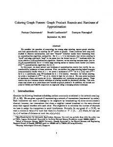
Algorithm 4.1 F irstF it(G) begin for i = 1 to n do assign smallest legal color to vi end-for end
Figure 4.1: First Fit Coloring Algorithm First Fit First Fit is the easiest and fastest of all greedy coloring heuristics. The algorithm is outlined in Figure 4.1. We first give some remarks about the presentation of coloring algorithms throughout this thesis. The graph to be colored, denoted by G, is given as a parameter to the heuristic. The number of vertices and edges of the input graph are denoted by n and m respectively. The steps in the algorithm are given in high level specification and enclosed between begin and end. The First Fit coloring algorithm is fed the set of vertices in some arbitrary order. The algorithm sequentially assigns each vertex the lowest legal color. First Fit has the advantage of being very simple and very fast. As for the quality of the coloring obtained, First Fit does not perform well in the worst-case. For some special graphs, the approximation ratio can be as high as n/4 [11]. On the average, however, it performs reasonably well. Grimmet and McDiamid [10] have given an average case analysis of its performance for the class of graphs known as random graphs. A random graph is a graph in which the probability of finding an edge between any two vertices is 1/2. They show that for random graphs, on the average, First Fit is expected to use no more than 2χ(G) colors. This result is achieved asymptotically as the graph gets large. Each step i in Algorithm 4.1 has operations proportional to the degree
CHAPTER 4. REVIEW OF GRAPH COLORING HEURISTICS
27
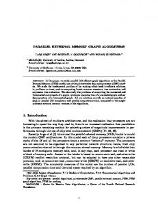
Algorithm 4.2 Greedy(G) begin U =V while U 6= ∅ do choose a vertex vi ∈ U according to a selection criterion assign smallest legal color to vi U = U − {vi } end-while end
Figure 4.2: General Greedy Coloring Scheme deg(vi ) of vertex vi . Thus the total time complexity is proportional to Pn
i=1 deg(vi ).
In other words, First Fit is an O(m)-time algorithm.
Degree based Ordering A better strategy than simply picking the next vertex from an arbitrary order is to use a certain selection criterion for choosing the vertex to be colored among the currently uncolored vertices. Such a strategy, depending on the nature of the selection criterion, has a potential for providing a better coloring than First Fit . We outline a general scheme of this approach in Figure 4.2, and call it a general greedy coloring scheme. In Algorithm 4.2, U is the set of uncolored vertices in each iteration. Initially it is set to be equal to V . A vertex v is selected using a certain criterion and colored. This colored vertex is then removed from U . This process of selecting, coloring and removing a vertex continues until the set of uncolored vertices U becomes empty. For graphs with low maximum degree, one can give an upper bound on the number of colors used by Algorithm 4.2. If ∆ is the maximum degree of the graph, then at each iteration of the while-loop, the vertex to be colored can have no more than ∆ neighbors. Hence, it must be possible to color this vertex with one of the colors 1, 2, . . . , ∆ + 1. Therefore, the greedy scheme
CHAPTER 4. REVIEW OF GRAPH COLORING HEURISTICS
28
uses at most ∆+1 colors. Note that First Fit belongs to this general scheme; it just selects the next vertex from some arbitrary ordering of the vertices. Hence, it also uses at most ∆ + 1 colors. Many strategies for selecting the next vertex to be colored have been proposed so far. Depending on the selection criterion used, we get a variety of coloring heuristics. In the following paragraphs we discuss some of the well-known, effective selection strategies. Largest Degree Ordering (LDO) Ordering the vertices by decreasing degree, proposed by Welsh & Powel [29], was one of the earliest ordering strategies. This ordering works as follows. Suppose the vertices v1 , v2 , . . . vi−1 have been chosen and colored. Vertex v i is chosen to be the vertex with the maximum degree among the set of uncolored vertices. Intuitively, LDO provides a better coloring than First Fit since during each iteration it chooses a vertex with the highest number of neighbors which potentially produces the highest color. Note that this heuristic can be implemented to run in O(m) time. Saturation Degree Ordering (SDO) SDO was proposed by Brelaz [3] and is defined as follows. Suppose that vertices v 1 , v2 , . . . vi−1 have been chosen and colored. Then at step i, vertex v i with the maximum saturation degree is selected. The saturation degree of a vertex is defined as the number of differently colored vertices the vertex is adjacent to. For example, if a vertex v has degree equal to 4 where one of its neighbors is uncolored, two of them are colored with color equal to 1, while the last one is colored with color equal to 3, then v has saturation degree equal to 2. While choosing a vertex of maximum saturation degree, ties are broken in favor of the vertex with the largest degree. Intuitively, this heuristic provides a better coloring than LDO since it first colors vertices most constrained by previous color choices. The heuristic can be implemented to run in O(n 2 ) time [3].
CHAPTER 4. REVIEW OF GRAPH COLORING HEURISTICS
29
Incidence Degree Ordering (IDO) A modification of the SDO heuristic is the incidence degree ordering introduced by Coleman and Mor´e [5]. This ordering is defined as follows. Suppose that vertices v 1 , v2 , . . . , vi−1 have been chosen and colored. Vertex vi is chosen to be a vertex whose degree is a maximum in the subgraph of G induced by the vertex set {v 1 , . . . , vi−1 }∪{vi }. In other words, a vertex vi with the maximum incidence degree is chosen at step i. The incidence degree of a vertex is defined as the number of its adjacent colored vertices. Note that it is the number of adjacent colored vertices and not the number of colors used by the vertices that is counted. The vertex v in the example of the above subsection has incidence degree equal to 3. Tie-breaking in IDO is as in the case of SDO. The IDO vertex ordering has the advantage that its running time is a linear function of the number of edges [16]. In other words, IDO is an O(m)-time algorithm. Independent Set Based Coloring Algorithms The degree-based heuristics discussed so far are the most commonly used sequential graph coloring heuristics. The reason for their common usage is their simplicity and relative high speed. In this subsection we consider greedy coloring heuristics based on finding an independent set. The observation in these heuristics is that vertices of an independent set can be assigned the same color. This approach reveals the close relationship between the graph coloring and independent set problems. The independent set problem and its related concepts have been introduced in Section 1.2. An independent set based coloring heuristic is presented in Figure 4.3. In this figure, IndependentSetAlgorithm is a routine that returns an independent set when provided with an input graph. The main algorithm works by repeatedly finding, coloring and removing an independent set. The set of uncolored vertices is denoted by U and G 0 is the graph induced by U . Initially G = G0 and U = V . I is set to be the independent set returned by IndependentSetAlgorithm with input G 0 . After the vertices in I are colored,
CHAPTER 4. REVIEW OF GRAPH COLORING HEURISTICS
30
Algorithm 4.3 IndependentSetBasedColoring(G) begin U =V G0 = G while G0 6= ∅ do I = IndependentSetAlgorithm(G0 ) color the vertices in I with a new color U =U −I G0 = graph induced by U end-while end Figure 4.3: Coloring by removing independent sets I is removed from U . The process is repeated on the graph G 0 induced by U and continues until G0 becomes empty. We note that the principle of successively extending a partial coloring is applied in Algorithm 4.3. Moreover, the coloring obtained is not iteratively improved. Hence we have classified this coloring heuristic under the category of greedy coloring heuristics. Both the quality and time complexity of Algorithm 4.3 is determined by the routine used for determining the independent set. The following paragraphs discuss some simple independent set finding heuristics. The heuristics find a maximal (and not a maximum) independent set in a graph. Finding a maximum independent set is NP-complete. (See Sections 1.2 and 1.3.) Greedy Independent Set The easiest method of finding a maximal independent set in a graph is the heuristic outlined in Figure 4.4. In Algorithm 4.4, U denotes the set of vertices under consideration and G 0 denotes the graph induced by U . The heuristic returns the independent set denoted by I. Initially U = V , I = ∅ and G0 = G. A vertex v is then chosen arbitrarily from U and augmented into the independent set I. Then the set X, which is the union of v and its neighbors N (v), is removed from U . This process
CHAPTER 4. REVIEW OF GRAPH COLORING HEURISTICS
31
Algorithm 4.4 GreedyIndependentSet(G) begin I =∅ U =V G0 = G while (G0 6= ∅) do choose a vertex v arbitrarily from U I = I ∪ {v} X = {v} ∪ N (v) U =U −X G0 = graph induced by U end-while return I end
Figure 4.4: Greedy Independent Set is repeated until the vertex set U becomes empty. Algorithm 4.4 performs (in terms of quality) badly in the worst case. On the average, however, it performs reasonably well [11]. Greedy independent set is specially useful for graphs with low maximum degree. If the degree of each vertex is at most ∆, then each step in Algorithm 4.4 will decrease the graph by no more than ∆ + 1 vertices. Hence, the n e. method will find an independent set of size at least d ∆+1
Minimum Degree Independent Set
In Algorithm 4.4, instead of pick-
ing an arbitrary vertex, it intuitively makes sense to choose a vertex of low degree in the graph G0 . This is because a minimum degree vertex entails a minimum size set of vertices to be removed (the set X is minimized). This enables the independent set finding process to continue longer resulting in a larger size independent set.
CHAPTER 4. REVIEW OF GRAPH COLORING HEURISTICS
4.2.2
32
Local Improvement Coloring Heuristics
Local improvement coloring heuristics start with some naive coloring of the graph. The vertices are then moved around between color classes iteratively with the hope of finding a better coloring. The iterative improvement stops when the algorithm decides no better coloring can be achieved. Thus, unlike in greedy coloring heuristics, a vertex may change its color several times during the course of a local improvement coloring algorithm. Local improvement coloring heuristics concentrate on two issues: finding a good objective function that accurately measures the quality of the current solution and finding a selection criterion for determining which vertices to move. Moves are, in general, considered to be good if they make progress towards a reduction in the number of colors used. There are various local improvement coloring heuristics in the literature. Examples include variants of Simulated annealing [20, 23] and Tabu search [6, 20]. In this section we present a local improvement coloring heuristic the idea of which has motivated one of our coloring algorithms discussed in Section 5.4. The coloring heuristic is called Iterated First Fit 1 and was proposed by Culberson [6]. Iterated First Fit Given a graph G = (V, E), let V = {v1 , . . . .vn } and π be a permutation of {1, . . . , n}. In Iterated First Fit, First Fit is applied iteratively where the ordering in each iteration is determined by a previous coloring. In other words, information obtained in a previous coloring is used to produce an improved coloring. The following result states that if we take any permutation in which the vertices of each color class are adjacent in the permutation, then applying First Fit once more will produce a coloring at least as good as what we had previously. 1
Culberson calls it Iterated Greedy.
CHAPTER 4. REVIEW OF GRAPH COLORING HEURISTICS
33
Lemma (Culberson) 4.1 Let C be a k-coloring of a graph G, and π a permutation of the vertices such that if C(v π(i) ) = C(vπ(m) ) = c, then C(vπ(j) ) = c for i < j < m. Then, applying the First Fit algorithm to the permutation π will produce a coloring C using k or fewer colors. Proof [6]: The proof is a simple induction showing that the first i color classes listed in the permutation will be colored with i or fewer colors. Clearly, the first color class listed will be colored with color 1. Suppose some element of the ith class requires color i + 1. This means that it must be adjacent to a vertex of color i. But by induction the vertices in the 1st to i − 1th classes used no more than i − 1 colors. Thus, the conflict has to be with a member of its own color class, but this contradicts the assumption that C is a valid coloring. 2 Clearly, the order of the vertices within the color classes cannot affect the next coloring, because the color classes are independent sets. It can easily be seen that if the permutation is such that the k color classes generated by a previous iteration of the algorithm are listed in order of increasing color, then applying the First Fit algorithm again will produce an identical coloring. Culberson suggests a number of heuristics by which the color classes can be reordered, satisfying the condition of Lemma 4.1. Being a local improvement heuristic, Iterated First Fit needs a mechanism for measuring progress between successive iterations. Clearly, coloring number could be used as a direct and accurate measure. It is easy to see that progress has been made whenever the coloring number is reduced. However, the algorithm may require hundreds or thousands of iterations on larger graphs before changes in coloring number are observed. To circumvent this, Culberson suggests the sum of the color values (remember the color of a vertex is just an integer) assigned to the vertices as an alternative measure of progress.
CHAPTER 4. REVIEW OF GRAPH COLORING HEURISTICS
34
Algorithm 4.5 P arallelColoring(G) begin U =V G0 = G while G0 6= ∅ do in parallel I = IndependentSetAlgorithm(G0 ) color the vertices in I U =U −I G0 = graph induced by U end-while end Figure 4.5: A Parallel Coloring Heuristic
4.3
Parallel Graph Coloring Heuristics
Developing a parallel algorithm, among other things, requires identification of operations that can be performed concurrently. One observes that the effective, ordering-based, greedy sequential coloring heuristics discussed so far are essentially breadth-first searches of the graph and, as such, do not lead to scalable, parallel heuristics. Independent set based coloring heuristics, on the other hand, are better suited for parallelization, since any independent set of vertices can be colored in parallel. Thus, a heuristic for determining an independent set in parallel could be adapted to a parallel coloring heuristic. A parallel independent set based coloring heuristic is given in Figure 4.5. In Algorithm 4.5, each of the stages within the while loop are executed in parallel in a synchronous fashion. Depending on how the independent set is chosen and colored, Algorithm 4.5 results in a number of variants, some of which are presented in the following sections.
CHAPTER 4. REVIEW OF GRAPH COLORING HEURISTICS
4.3.1
35
Parallel Maximal Independent Set (MIS)
The problem of determining an independent set in parallel has been the focus of much theoretical research. One approach, that has been successfully analyzed by Luby [21], is to determine an independent set I based on a Monte Carlo rule as follows. 1. For each vertex v ∈ U determine a distinct, random number ρ(v) 2. v ∈ I ⇔ ρ(v) > ρ(ω), ∀ω ∈ adj(v) In Luby’s algorithm (Algorithm 4.6), this initial independent set is augmented to obtain a maximal independent set. In this algorithm, after the initial independent set is found, the set of vertices adjacent to a vertex in I, the neighbor set N (I), is determined. The union of these two sets is deleted from U , the subgraph induced by this smaller set is constructed, and the Monte Carlo step is used to choose an augmenting independent set. This process is repeated until the candidate vertex set is empty and a maximal independent set (MIS) is obtained. Luby has described a parallel version of his algorithm. He has shown that an upper bound for the expected time to compute an MIS by this algorithm on a CRCW PRAM is EO((∆ + 1) log(n)), where ∆ is maximum degree of G and n is the number of vertices. Luby’s algorithm can be adapted to a graph coloring heuristic by using it to determine a sequence of distinct maximal independent sets and coloring each MIS with a different color. We call this coloring method Parallel MIS coloring. Parallel MIS will color a graph with maximum degree ∆ in expected time EO((∆ + 1)log(n)).
4.3.2
Jones-Plassmann
Jones and Plassmann [16] state the following. “One major deficiency of the parallel MIS coloring approach on distributed memory parallel computers is that each new choice of random numbers in the MIS algorithm requires a global synchronization of the processors. A second problem is that each new
CHAPTER 4. REVIEW OF GRAPH COLORING HEURISTICS
36
Algorithm 4.6 Luby − M IS(G) begin I =∅ U =V G0 = G while (G0 6= ∅) do Choose an independent set I 0 in G0 using the Monte Carlo rule described I = I ∪ I0 X = I 0 ∪ N (I 0 ) U =U −X G0 = graph induced by U end-while end
Figure 4.6: Luby’s Monte Carlo algorithm for determining a MIS choice of random numbers incurs a great deal of computational overhead, because the data structures associated with the random numbers must be recomputed.” They propose an asynchronous parallel heuristic for a distributed memory parallel computer that avoids both of these drawbacks. Their heuristic is based on a message-passing model. According to them, the first drawback, global synchronization, is eliminated by choosing the independent random numbers only at the beginning of the heuristic. With this modification, the interprocessor communication can proceed asynchronously once these numbers are determined. The second drawback, computational overhead, is alleviated because with this heuristic, once a processor knows the values of the random numbers of the vertices to which it is adjacent, the number of messages it needs to wait for can be computed and stored. Likewise, each processor computes only once the processors to which it needs to send a message once one of its vertices is colored. To make comparison with the parallel MIS algorithm easier, we present
CHAPTER 4. REVIEW OF GRAPH COLORING HEURISTICS
37
Algorithm 4.7 Jones − P lassmann(G) begin U =V while(|U | > 0) do for all vertices v ∈ U do in parallel I = {v such that w(v) > w(u)∀ neighbors u ∈ U } for all vertices v 0 ∈ I do in parallel assign the smallest legal color to v 0 end-for end-for U =U −I end-while end
Figure 4.7: High-level, Jones-Plassmann coloring algorithm the Jones-Plassmann algorithm at a higher level (Figure 4.7). This presentation does not assume any specific parallel programming model. In Algorithm 4.7, w(v) denotes the random number (weight) assigned to vertex v at the beginning of the heuristic. We see that the algorithm proceeds very much like the parallel MIS algorithm, except that it does not find a maximal independent set at each step. It just finds an independent set in parallel using Luby’s Monte Carlo rule, choosing vertices whose weights are local maxima. The other difference is that the vertices in the independent set found are not assigned the same new color, as they are in the MIS algorithm. Instead, the vertices are colored individually using the smallest consistent color, the smallest color that has not already been assigned to a neighboring vertex. This procedure is repeated using the coloring method of Figure 4.5 until the entire graph is colored. In choosing vertices with local maximum weight, Jones-Plassmann algorithm uses the unique vertex number to tie-break in the unlikely event of neighboring vertices getting the same random number. Jones and Plassmann provide an analysis of the expected running time
CHAPTER 4. REVIEW OF GRAPH COLORING HEURISTICS
38
of their heuristic for bounded degree graphs (graphs with maximum degree ∆) under the PRAM computational model. By this analysis, for fixed ∆, they improve Luby’s bound of EO(log(n)) to EO(log(n)/ log log(n)). They have also described how their asynchronous parallel coloring heuristic can be combined with effective sequential heuristics on distributed memory parallel computers. They achieve this by first partitioning the vertices of the input graph across p processors in a distributed memory parallel computer. The combined approach consists of two phases: an initial, parallel phase as described by Algorithm 4.7, followed by a local phase that uses some good sequential coloring heuristic. We shall elaborate this combined approach in Chapter 5.
4.3.3
Largest Degree First (LDF)
The Largest Degree First [1] algorithm is basically very similar to the JonesPlassmann algorithm. The only difference is that instead of using random weights to create the independent sets, each weight is chosen to be the degree of the vertex in the graph induced by the uncolored vertices. Random numbers are only used to resolve conflicts between neighboring vertices having the same degree. Vertices are thus not colored in random order, but rather in order of decreasing degree. LDF aims to use fewer colors than the Jones-Plassmann algorithm. This is so because a vertex with i colored neighbors requires at most color i + 1 and the LDF algorithm aims to keep the maximum value of i as small as possible throughout the computation. Therefore, LDF has a tendency of using smaller number of colors than Jones-Plassmann.
Chapter 5
New Parallel Graph Coloring Heuristics 5.1
Introduction
In their work entitled “A comparison of parallel graph coloring algorithms”, Allwright et al. [1] have experimentally demonstrated the performance of the parallel coloring algorithms presented in the previous chapter. They have implemented Parallel MIS, Jones-Plassmann and LDF coloring algorithms on both SIMD and MIMD parallel architectures. Their findings indicate that LDF and Jones-Plassmann use almost the same coloring time and are generally faster than Parallel MIS. In terms of quality of coloring, their results indicate that LDF uses fewer number of colors than Jones-Plassmann and Jones-Plassmann uses fewer colors than Parallel MIS. However, Allwright et. al report that they did not get any speedup for all the algorithms. Moreover, they could not experiment on graphs of very large size due to memory limitation. Jones and Plassmann [16] do not report on obtaining speedup either. They state that “the running time of the heuristic is only a slowly increasing function of the number of processors used”, where the heuristic referred to is a combination of their asynchronous parallel heuristic and local sequential coloring heuristics. Moreover, this combined coloring heuristic of Jones and Plassmann is based on a distributed-memory architecture.
39
CHAPTER 5. NEW PARALLEL GRAPH COLORING HEURISTICS 40 Therefore, developing parallel, shared-memory programming based graph coloring heuristics that yield good speedup is interesting. The main reason for choosing shared-memory programming is to utilize effective sequential coloring heuristics and incrementally parallelize them without incurring huge computational overhead. This chapter presents the parallel graph coloring algorithms developed in this work. The basic parallelization technique applied is partitioning. Partitioning, as a parallelization strategy, consists of (1) breaking up the given problem into p independent subproblems of almost equal sizes, and then (2) solving the p subproblems concurrently using p processors. We use the parallel machine model PRAM, discussed in Section 3.2.1, for the analyses of the algorithms. In the analyses of some of the algorithms, we use the probabilistic concept expected value, defined in Section 2.5.1. Our emphasis is more on speed than quality of coloring. Therefore, First Fit is the coloring heuristic the reader encounters often in this chapter. First Fit and other greedy sequential coloring heuristics were discussed in Section 4.2.1. In this work, partitioning as a parallelization technique has been applied in two different ways to the graph coloring problem. This chapter is organized based on these two ways of applying the partitioning technique. Section 5.2 shows the application of the graph partitioning problem in breaking the graph coloring problem into a number of independent subproblems. In Section 5.3 we show how simple block partitioning can be used in breaking the graph coloring problem into several, not necessarily independent, subproblems. We show that inconsistencies that result due to the interdependence of the subproblems can be resolved later using a “conflictresolving” stage. In Section 5.4 we show how the quality of coloring obtained using block partitioning can be improved. The improvement method is based on a twophase coloring strategy. Each of the coloring phases is performed in parallel
CHAPTER 5. NEW PARALLEL GRAPH COLORING HEURISTICS 41 using block partitioning. We show that the second phase, in addition to improving the quality of coloring, results in fewer “conflicts”. Section 5.5 discusses how the two partitioning approaches can be combined to yield a cumulative improved result.
5.2
Graph Partitioning Approach
Our first approach of breaking the graph coloring problem into several subproblems is using the graph partitioning problem. The objective of the graph partitioning problem is to partition the vertices of a graph in p roughly equal parts such that the number of edges connecting vertices in different parts is minimized. For our purpose the partitioning is done across the p processors available. If the graph partitioning problem is solved effectively, that is, with nearly equal number of vertices per processor and only very few edges connecting vertices in different processors, then the graph coloring problems defined by the local vertices of each processor can be solved concurrently and the potential for good speedup is clear. In this section we look in to this idea more closely and present the first parallel coloring heuristic.
5.2.1
Definitions and Notations
Assume that the vertices of the graph G = (V, E) are partitioned into p sets as {V1 , . . . , Vp }. Let the function π : V → {1, . . . , p} return the number of the partition to which each vertex belongs. We define the set of shared edges E S to be the edge set E S ⊆ E where
edge (v, w) ∈ E S ⇔ π(v) 6= π(w) and the set of shared vertices to be the
vertex set V S , where a vertex is in this set if and only if the vertex is an
endpoint for some edge in E S . Let the set of local vertices, denoted by V L , be the set V − V S , and let
Vi L denote the vertex set V L ∩ Vi . Thus,
S
Vi L = V L .
Let Gi and GL denote the graphs induced by the vertex sets V i L and V L
respectively and let GS be the graph obtained by deleting all the edges (but NOT the vertices) of GL from G.
CHAPTER 5. NEW PARALLEL GRAPH COLORING HEURISTICS 42
5.2.2
The Algorithm
We make the following two crucial observations. The coloring algorithm follows directly from these results. Lemma 5.2.1 Let σi be a coloring for Gi . A coloring σ for the graph GL can be obtained by letting σ(v) = σi (v) where v ∈ Vi L , for each i = 1, . . . , p.
Proof : By definition, the vertex sets V 1 L , . . . , Vp L are equivalent classes of the vertex set VL . Hence, the subgraphs Gi (for i = 1, . . . , p) are connected components of GL . This implies that colorings of the subgraphs G i (for i = 1, . . . , p) can be pieced together as-they-are to provide a coloring for GL . 2 Lemma 5.2.2 A coloring for GL is a partial coloring for GS and can be extended to a coloring for G. Proof : The vertices in the graph GS are of two kinds: those that belong to V L and those that belong to V S . The vertices from V L are already colored. Coloring the vertices in V S , consistent with the colors assigned to vertices in V L , provides a coloring for graph G. 2 Lemmas 5.2.1 and 5.2.2 immediately suggest a parallel coloring scheme that works in two phases. During the first phase, the p local graphs are colored in parallel by p processors, each processor using any sequential coloring algorithm. In the second phase, GS , the graph that remains when all the edges of the local graphs are removed, is colored using any parallel coloring heuristic. The coloring scheme based on this principle is outlined in Figure 5.1. Scheme 5.1 yields a parallel coloring algorithm by specifying the algorithms to be used in Phases 1 and 2 . One combination of choices could for
CHAPTER 5. NEW PARALLEL GRAPH COLORING HEURISTICS 43 Scheme 5.1 GraphP artitionBasedColoring(G, p) begin 1. Partition G into p parts and determine V i L , V S and Gi for i = 1 to p do in parallel Color Gi using some sequential coloring algorithm end-for 2. Color the remaining vertices in V S consistently using some parallel coloring heuristic end
Figure 5.1: Graph Partition Based Coloring Scheme instance be using First Fit in Phase 1 and the Jones-Plassmann algorithm (Algorithm 4.7) in Phase 2. In fact the basic idea in Scheme 5.1 is inspired by the work of Jones and Plassmann [16]. They have shown that the asynchronous parallel coloring heuristic, Algorithm 4.7, can be combined with local sequential coloring heuristics using the same idea of graph partitioning. The difference between their method and ours lies in the order in which the two phases are performed. They show that coloring of the shared graph G S can be done before coloring of the local graphs. Our method is better for the following two reasons. Firstly it is more suitable for SMP and secondly it fits very well into the general parallel coloring method of Algorithm 4.5. In Scheme 5.1, since the Gi ’s are connected components of GL , if we consider each graph Gi as a “node”, the set composed of these nodes is an independent set in G. Scheme 5.1 is thus equivalent to a one-iteration variant of Algorithm 4.5, where an “independent set” is found, colored, removed from the graph and finally the vertices that remain after such removal are colored. The performance, both in terms of speed and quality, of Scheme 5.1 is highly dependent on the partitioning step. Graph partitioning is a well studied and important problem by itself. The problem is known to be NPcomplete. The study of this problem is out of the scope of this work.
CHAPTER 5. NEW PARALLEL GRAPH COLORING HEURISTICS 44 For some sparse graphs1 , the partitioning step in Scheme 5.1 yields a partition in which |E S | � |E| (the percentage of edges whose end points are in different parts is low). For such graphs, Scheme 5.1 is effective and Phase 2 can even be done sequentially without producing significant increase in the overall time required. We finally comment on how our use of partitioning as a parallelization technique in Scheme 5.1 differs from the standard partitioning strategy. In the standard case, the union of the independent subproblems is equal to the original whole problem. In our case, this is not so. The difference between the whole problem and the union of the subproblems is the problem defined by GS . By trying to minimize the size of E S in the partitioning step, our parallelization technique is made as close to the standard as possible.
5.3
Block Partitioning Approach
The partitioning strategy of Scheme 5.1 calls for the solution of another NPcomplete problem. Moreover, all graphs can not be partitioned effectively. For some graphs the size of E S can be as big as E itself. In this section we propose an alternative partitioning method, called simple block partitioning. By block partitioning is meant dividing the vertex set (given in an arbitrary order) into p successive blocks of equal size. No effort is made to minimize the number of edges whose end points belong to different blocks. Such edges, the end points of which belong to different blocks, are said to be crossing edges. Obviously, because of the existence of crossing edges, the coloring subproblems defined by the blocks in a block partitioning are not independent. That is to say, coloring the vertices of one block can not necessarily be done concurrently with coloring of the vertices of another block without resulting in inconsistency. 1
Sparse graphs are graphs where the number of edges is much smaller than the square of the number of vertices, more on this in Chapter 6
CHAPTER 5. NEW PARALLEL GRAPH COLORING HEURISTICS 45
Algorithm 5.2 BlockP artitionBasedColoring(G, p) begin 1. Partition V into p equal blocks b1 . . . bp , where |bi | = |V |/p = n/p for i = 1 to p do in parallel for j = 1 to n/p do assign the smallest legal color to vertex v j ∈ bi end-for end-for 2. for i = 1 to p do in parallel for j = 1 to n/p do for each neighbor u of vj ∈ bi do if color(vj ) = color(u) then store min {u, vj } in an array A end-if end-for end-for end-for Color the vertices in A sequentially end
Figure 5.2: Block Partition Based Coloring Algorithm
CHAPTER 5. NEW PARALLEL GRAPH COLORING HEURISTICS 46
5.3.1
The Algorithm
Our strategy in this second approach of partitioning is to solve the original problem in two phases. In the first phase, the input vertex set is divided into p blocks of equal size and the vertices in each block are colored in parallel using p processors. The p processors operate in a synchronous fashion. That is, at each time unit tj , each processor colors vertex vj in its respective block. In doing so, two processors may simultaneously be attempting to color vertices that are adjacent to each other. This may result in an invalid coloring. In the second phase, the vertex set is block partitioned as in Phase 1 and each processor checks whether its vertices are legally colored. If a conflict is discovered, one of the endpoints of the edge in conflict is stored in a table. Finally the vertices in this table are colored sequentially. The details of the parallel coloring algorithm based on this strategy are given in Figure 5.2.
5.3.2
Results
In this section we present some results regarding Algorithm 5.2. We call the coloring obtained at the end of Phase 1 in Algorithm 5.2 a pseudo coloring to indicate that it may contain conflicts. The input graph G = (V, E) in Algorithm 5.2 has n vertices, m edges, and a maximum degree of ∆. The algorithm uses p processors. Our first result shows that Phase 1 in Algorithm 5.2 provides a nearly linear speedup. Lemma 5.3.1 Phase 1 of Algorithm 5.2 pseudo colors the input graph in O(∆n/p) time using O(m) operations on the CREW PRAM. Proof : In coloring the vertices of the blocks in parallel, the end points of some crossing edges may be colored concurrently. Such vertices may end up getting the same color. Thus, at the end of Phase 1 some vertices may be illegally colored and it follows that the graph is pseudo colored. Moreover, two vertices being colored concurrently by two processors may have
CHAPTER 5. NEW PARALLEL GRAPH COLORING HEURISTICS 47 a common neighbor, the color of which has to be accessed simultaneously. Thus, the PRAM model required is CREW. We now turn to the complexity bounds. We first take the parallel time bound. Phase 1 of Algorithm 5.2 consists of n/p parallel steps. The number of operations in each parallel step is proportional to the degree of the vertex under investigation. The degree of each vertex is bounded from above by ∆. Thus, T 1 , the parallel time used by Phase 1, is T1 = O(∆n/p). As for the number of operations the following holds. W1 =
Pp
i=1
Pn/p
j=1,vj ∈bi
deg(vj ) = O(m). 2
The second result gives an upper bound on the expected number of edges whose end points are assigned the same color at the end of Phase 1 of Algorithm 5.2. Such edges are said to be in conflict and the cardinality of the set of edges in conflict is denoted by K. The result shows that K is bounded from above by (δp) where δ is the average degree in the graph G. Lemma 5.3.2 The expected number of conflicts at the end of Phase 1 of Algorithm 5.2 is EO(δp). Proof : Let e = (u, v) be an edge from E. Let P r[X, t j ] denote the probability that the set of vertices X, containing one or more vertices, is colored at time unit tj , where 1 ≤ j ≤ n/p. Clearly, P r[{u}, t j ] =
1 n/p
= p/n.
Similarly, P r[{v}, tj ] = p/n. The probability that u and v are colored at time unit tj is therefore obtained as follows. P r[{u, v}, tj ] = P r[{u}, tj ] × P r[{v}, tj ] = p/n × p/n = p2 /n2
(5.1)
The probability that u and v are colored at some same time unit is thus n/p X
p2 /n2 = (n/p)(p2 /n2 ) = p/n
(5.2)
j=1
Let S denote the number of edges the end points of which are colored concurrently. Using 2.1, the expected value of S is E[S] =
X (u,v)∈E
p/n =
mp = δp n
(5.3)
CHAPTER 5. NEW PARALLEL GRAPH COLORING HEURISTICS 48 The expression in Equation 5.3 is obviously an upper limit on the expected number of conflicts. Thus, E[K] = O(δp)
(5.4) 2
The following is our final result about Algorithm 5.2. In this result, we introduce a graph attribute called relative sparsity r, defined as r =
n2 m.
The attribute r indicates how sparse the graph is, the higher the value of r, the sparser the graph is. The following Lemma states that overall, for some graphs, Algorithm 5.2 provides an almost linear speedup compared to sequential First Fit coloring. √ Lemma 5.3.3 If p = O( r), then Algorithm 5.2 legally colors the graph in EO(∆n/p) time on a CREW PRAM. Proof : From Lemma 5.3.1, the time required by Phase 1 is T 1 = EO(∆n/p). Phase 2 has this time requirement plus the time it takes to sequentially color the conflicting vertices. That is, T 2 = EO(∆n/p)+EO(∆K) where K is the number of conflicts at the end of Phase 1. From Lemma 5.3.2 E[K] = O(δp). In other words, T2 = EO(∆n/p) + EO(∆δp). T2 is determined by how (n/p) compares with (δp). We investigate two cases. Case 1 ((n/p) � (δp)) √ n/p � δp ⇐⇒ n/p � (m/n)p ⇐⇒ n2 /m � p2 ⇐⇒ r � p2 ⇐⇒ p = O( r) (5.5) √ Thus, if p = O( r), then T2 = EO(∆n/p) and the overall time complexity of Algorithm 5.2 is T = T1 + T2 = EO(∆n/p). Case 2 ((n/p) � (δp))
√ Using similar derivations as in Case 1, if p = Ω( r), then T2 = EO(∆δp) and the overall time complexity of Algorithm 5.2 is T = T 1 +T2 = EO(∆δp). Furthermore, Phase 2 resolves all the conflicts that are inherited from Phase 1 and therefore the coloring at the end of Phase 2 is legal. Both Phase
CHAPTER 5. NEW PARALLEL GRAPH COLORING HEURISTICS 49 1 and 2 require concurrent read capability and thus the required PRAM is CREW. This completes our proof. 2
5.4
Improved, Block Partition Based Coloring
In this section we improve on the performance of the block partitioning based coloring of Algorithm 5.2. In doing so we achieve two results: reduction in the number of conflicts that arise due to crossing edges and reduction in the number of colors used. The improvement method is based on the idea behind Culberson’s Iterated First Fit (Section 4.2.2). From Lemma 4.1, we recall that if First Fit coloring is reapplied on a graph where the vertex set is ordered in such a way that vertices belonging to one color class in a previous coloring are listed consecutively, the new coloring is better or at least as good as the previous coloring. There are many ways in which the vertices of a graph can be arranged satisfying the condition of Lemma 4.1. One such ordering is a reverse color class ordering [6]. In this ordering, the vertices in the highest color class are listed first, followed by the vertices of the next highest color class, and so on, and the vertices of color class 1 are listed finally. This ordering has a good potential for an improved coloring since the new coloring proceeds by first coloring vertices that have been difficult to color in the previous coloring. By difficult to color we mean that it was not possible to color the vertex with a low color value.
5.4.1
The Algorithm
Once again our improved coloring works in two phases. The first phase is the same as Phase 1 of Algorithm 5.2. The vertex set is divided into p successive blocks and the blocks are colored in parallel. As we have seen in the previous section, this coloring may contain some conflicts and hence is a pseudo coloring. Let the coloring number used by this phase be ColN um. During the second phase, the pseudo coloring of the first phase is used to get a reverse color class ordering of the vertices. The second phase consists
CHAPTER 5. NEW PARALLEL GRAPH COLORING HEURISTICS 50 Algorithm 5.3 ImprovedBlockP artitionBasedColoring(G, p) begin 1. Partition V into p equal blocks b1 . . . bp , where |bi | = |V |/p = n/p for i = 1 to p do in parallel for j = 1 to n/p do assign the smallest legal color to vertex v j ∈ bi end-for end-for { coloring number = ColNum } { At this point we have pseudo independent sets ColorClass(1) . . . ColorClass(ColNum) } 2. for k = ColN um down to 1 do Partition ColorClass(k) into p equal blocks b 01 . . . b0p for i = 1 to p do in parallel for j = 1 to |ColorClass(k)|/p do assign the smallest legal color to vertex v j ∈ b0i end-for end-for end-for Conflict removing step (as Phase 2 of Algorithm 5.2) end
Figure 5.3: Improved, Block Partition Based Coloring Algorithm of ColN um steps. In each step i, the vertices of color class ColN um − i − 1 are colored afresh in parallel. The parallel coloring is done using the same method of block partitioning as in Phase 1. The algorithm using these two phases is described in Figure 5.3. Each color class at the end of Phase 1 is a pseudo independent set. Hence block partitioning of the vertices of each color class results in only a few crossing edges. In other words, the number of conflicts expected at the end of Phase 2 (K2 ) is much smaller than the number of conflicts at the end of Phase 1 (K1 ). Thus, in addition to improving the quality of coloring, Phase 2 is expected to provide a significant reduction in the number of conflicts. Note that a conflict removing step is included at the end of Phase 2 in Algorithm 5.3 to ensure that any remaining conflicts are removed.
CHAPTER 5. NEW PARALLEL GRAPH COLORING HEURISTICS 51
5.4.2
Results
The following result shows that Phase 2 reduces the number of conflicts from Phase 1 by a factor of (∆δp/m). To get a feeling of this reduction factor, consider an example where m = 2, 000, 000, ∆ = 100, δ = 40 and p = 20. The reduction factor is 100 ∗ 40 ∗ 20/2, 000, 000 = 0.04. Lemma 5.4.1 The expected number of conflicts at the end of Phase 2 of Algorithm 5.3 is EO(K1 ∆δp/m), where K1 is the number of conflicts inherited from Phase 1. Proof : Consider a color class c from the coloring obtained at the end of Phase 1 of Algorithm 5.3. Let the graph induced by the vertices of this color class be G0 = (V 0 , E 0 ) with n0 = |V 0 |, m0 = |E 0 |. Let e = (u, v) be an edge from E 0 . At the end of Phase 2, for u and v to be in conflict the following two conditions should be met. 1. u and v were invalidly colored in Phase 1, and 2. u and v are colored concurrently in the block partitioning of color class c. Let P r[condj ] be the probability that condition j is true. From Lemma 5.3.2, the expected number of conflicts at the end of Phase 1 is O(δp). The total number of edges in the original graph is m. Therefore, P r[cond1 ] = O(δp/m)
(5.6)
Similar arguments as in Lemma 5.3.2 can be applied to get the following. n0 /p
P r[cond2 ] =
X
p2 /n02 = p/n0
(5.7)
j=1
Observe that the graph G0 is induced by a psuedo independent set. This 0
means that the average degree in G0 , δ = m0 /n0 is much smaller than δ = m/n. Thus, the expected number of conflicts in color class c at the end of Phase 2 is given by E[K 0 ] = O(
X (u,v)∈E 0
(δp/m)(p/n0 )
(5.8)
CHAPTER 5. NEW PARALLEL GRAPH COLORING HEURISTICS 52 m0 p2 δ ) mn0 = O((δp)(δp/m))
(5.10)
= O(K1 (δp/m))
(5.11)
= O(K12 /m)
(5.12)
= O(
(5.9)
Equation 5.11 expresses the expected number of conflicts in one color class. There are at most ∆ + 1 color classes at the end of Phase 1. Therefore the total number of conflicts at the end of Phase 2 is expected to be E[K2 ] = O(
K1 ∆δp ) = O(K12 ∆/m) m
(5.13)
This completes our proof. 2
5.5
Hybrid
We have seen two basic methods of decomposing the the graph coloring problem. These are the graph partitioning approach of Section 5.2 and the block partitioning approaches of Section 5.3 and Section 5.4. The graph partitioning approach has the advantages that • for easily partitionable graphs, it has a good potential for speedup • it can be effectively combined with good sequential coloring heuristics • it is free of any conflict resolving phase Its disadvantages are that • it requires solving the NP-complete graph partitioning problem • dense graphs can not be partitioned effectively The block partitioning approach has the advantages that • it is simple
CHAPTER 5. NEW PARALLEL GRAPH COLORING HEURISTICS 53 Algorithm 5.4 HybridColoring(G, p) begin 1. Partition G into p parts and determine V i L , V S and Gi , GS for i = 1 to p do in parallel Color Gi using some sequential coloring algorithm end-for 2. BlockPartitionBasedColoring(G S ,p) end
Figure 5.4: Hybrid Coloring Algorithm • it is fast • it can be used for both sparse and dense graphs Its disadvantages are that • it requires a conflict resolving phase. • it has more communication overhead The two approaches can be combined to provide a cumulative improved result. One combination is achieved by using Algorithm 5.2 in Phase 2 of Scheme 5.1. In words, start with graph partitioning and color the resulting local graphs in parallel. Then use block partitioning to color the remaining shared graph in parallel in consistency with the coloring of the local graphs. This algorithm is given in Figure 5.4. If a better quality coloring is desired, step 2 of Algorithm 5.4 can be replaced by Algorithm 5.3.
Chapter 6
Implementation We have implemented the algorithms presented in Chapter 5 in Fortran 90 on an SGI CRAY Origin 2000 parallel computer using SMP model. We used OpenMP to obtain fine-grained parallelization. In this chapter we discuss implementation details such as the data structure used to store a graph and the procedure used to determine the smallest legal color for a vertex. A brief description of the Origin 2000 and an introduction to OpenMP is also provided.
6.1
Graph Representation and Storage
A graph G = (V, E) with |V | = n, |E| = m can be represented in two basic ways. The first representation is called an adjacency matrix representation. The adjacency matrix of G is an n × n matrix A such that a ij = 1 ⇔ (vi , vj ) ∈ E. The ith row of the matrix is thus an array of size n which has 1 in the jth position if there is an edge leading from v i to vj , and 0 otherwise. If the number of edges m is much smaller than n 2 , the graph is said to be sparse, otherwise it is called dense. Most of the entries in the adjacency matrix of a sparse graph will be 0s. Instead of having an explicit representation for all the 0s, one can link the actual number of 1s in a linked list. This is the second way of representing a graph and is called the adjacency list representation. In this representation, each vertex is associated with a linked list consisting of all the edges adjacent
54
CHAPTER 6. IMPLEMENTATION
55
to this vertex. The whole graph is represented by an array of lists. Each entry in the array includes the label of the vertex, and a pointer to the beginning of its list of edges. It is customary to store an n×n dense matrix in an n×n array. However, if the matrix is sparse, storage is wasted because a majority of the matrix elements are zero and need not be stored explicitly. For sparse matrices, it is common practice to store only the nonzero entries and to keep track of their locations in the matrix. A variety of storage schemes are used to store and manipulate sparse matrices [19]. These specialized schemes not only save storage but also yield computational savings. In our implementation, the adjacency structure of the graph is stored using the compressed storage format (CSR). CSR is a widely used scheme for storing sparse graphs. In this format, the adjacency structure of a graph is represented using two arrays vertexArray and edgeArray. For example, consider a graph with n vertices and m edges. In the CSR format, this graph is stored using the arrays vertexArray[n+1] and edgeArray[2m]. Note that the reason edgeArray is of size 2m is because for each edge between vertices v and u we actually store (v, u) as well as (u, v). The adjacency structure of the graph is stored as follows. Assuming that vertex numbering starts from 0 then the adjacency list of vertex i is stored in array edgeArray starting at index vertexArray[i] and ending at (but not including) index vertexArray[i + 1]. That is, for each vertex i, its adjacency list is stored in consecutive locations in the array edgeArray, and the array vertexArray is used to point to where it begins and where it ends.
6.2
Determination of Smallest Legal Color
In our implementations, the data structure used to store the colors assigned to the vertices of a graph is an integer array. That is, color[i] stores the color assigned to vertex i. In determining the smallest legal color for a vertex, we use a working array called used, of size k for a k-colorable graph. Let us say we want to
CHAPTER 6. IMPLEMENTATION
56
assign the smallest legal color to vertex v. For each neighbor u of v, used[u] is set to be equal to v. Then the array used is scanned from left to right, starting at index equal to 1 up to the number of colors used so far, until the first entry with value different from v is obtained. If such a search finds an index less than or equal to the number of colors used so far, this index is taken to be the color of vertex v. If no such index is found, a new color is created and assigned to vertex v.
6.3
Graph Partitioning Program
In Chapter 5 an algorithm that requires an effective solution for the graph partitioning problem was presented. One of the successful algorithms proposed for the graph partitioning problem is the multi level graph partitioning scheme [18]. In our implementation, we used Metis version 3.0.3, a graph partitioning program based on this scheme [17], to partition a graph into p parts.
6.4
OpenMP
OpenMP supports two basic flavors of parallelism: coarse-grained and finegrained. In the former case, the program is broken into segments (threads) that can be executed in parallel and barriers are used to re-synchronize execution at the end. In the latter case, the iterations of DO loops are executed in parallel. An OpenMP Fortran Application Program Interface (API) is available on our target computer, the Origin 2000. A program written with the OpenMP Fortran API begins executing as a single process, called the master thread of execution. The master thread executes sequentially until the first parallel construct is encountered. At this point, the master thread creates a team of threads, and the master thread becomes the master of the team. This is called forking. The statements in the program that are enclosed by the parallel construct are executed in parallel by the threads in the team. Upon completion of the parallel
CHAPTER 6. IMPLEMENTATION
57
construct, the threads in the team synchronize and only the master thread continues execution. We call this joining. Parallel region construct. In the OpenMP Fortran API, the PARALLEL and END PARALLEL directive pair is the fundamental parallel construct defining a parallel region. This directive pair has the following format: !$OMP PARALLEL [clause[[,] clause] . . . ] block !$OMP END PARALLEL As the format depicts, different clauses might be added to the PARALLEL directive. The most important ones are PRIVATE and SHARED, in which variables are defined to be either private to a thread or shared among threads in a team. The block denotes a structured block of Fortran statements. It is illegal to branch into or out of the block. The END PARALLEL directive denotes the end of the parallel region. There is an implicit barrier at this point. Work-sharing constructs A work-sharing construct divides the execution of the enclosed code region among the members of the team that encounter it. It must be enclosed within a parallel region in order for the directive to execute in parallel. A work-sharing directive does not launch new threads, and there is no implied barrier on entry to a work-sharing construct. The DO and END DO directive pair is the most natural example of a work-sharing construct. The DO directive specifies that the iterations of the immediately following DO loop should be executed in parallel. The loop that follows a DO directive cannot be a DO WHILE or a DO loop without loop control. The iterations of the DO loop are distributed across threads that already exist. The format of this directive is as follows.
CHAPTER 6. IMPLEMENTATION
58
!$OMP DO [clause[[,] clause] . . . ] do-loop !$OMP END DO [NOWAIT] If NOWAIT is specified, threads do not synchronize at the end of the parallel loop. Threads that finish early proceed straight to the instructions following the loop without waiting for the other members of the team to finish the DO directive. Combined parallel work-sharing constructs The PARALLEL DO directive provides a shortcut form for specifying a parallel region that contains a single DO directive. The format of this directive is: !$OMP PARALLEL DO [clause[[,] clause] . . . ] do-loop !$OMP END PARALLEL DO
6.5
Origin 2000
The Cray Origin 2000 parallel machine we used consists of 128 MIPS R10000 processors interconnected as a hypercube. The machine provides cachecoherent, non-uniform memory access. Each processor has 4 MB primary cache and 192 MB local memory. Processors can read data only from primary cache. If the required data is not present in the primary cache, a cache miss is said to have occurred. Therefore, references to locations in the remote memory of another processor take substantially longer to complete than references to locations in local memory. Cache misses adversely affect program performance.
6.6
Data Distribution
To obtain good performance in parallel programs it is important to schedule computation and to distribute the data across the underlying processors and memory modules, ensuring that most cache misses are satisfied from local
CHAPTER 6. IMPLEMENTATION
59
rather than from remote memory. If the misses are to data that is referenced primarily by a single processor, then data placement may be able to convert remote references to local references, thereby reducing the latency of the miss. Explicit data distribution is one method for data placement. The distribution can either be regular or reshaped. The Power Fortran compiler we used provides a mechanism for data distribution through the directive DISTRIBUTE. This directive is not part of OpenMP, but an extension provided by SGI. The !$SGI DISTRIBUTE directive determines the data distribution for an array. It has the following format. !$SGI DISTRIBUTE array (dist1, dist2) The name of the array is specified by array. The parameters dist1 and dist2 specify the type of distribution for each dimension of the named array. The number of dist arguments specified must be equal to the number of array dimensions. A dist parameter can be one of the following: a. BLOCK b. CYCLIC c. An asterisk (*), indicating that the dimension is not distributed. Figure 6.1 demonstrates the difference between block and cyclic distribution. A block ditribution is one that partitions the elements of the dimension of size N into p blocks (one per processor), with each block of size B = dN/pe. A cyclic[K] distribution partitions the elements of the dimension into pieces of size K each and distributes them sequentially across the processors. The following is an example of the use of data distribution. Let A(x,y) be a two dimensional integer array. Let us say that we want to increment the contents of A by 1. The parallelized Fortran code for this is given in Figure 6.2. The parallel loop in Figure 6.2 benefits greatly from the distribution
60
CHAPTER 6. IMPLEMENTATION
Block Distribution P1
P2
P3
B
B
B
Pp ...
B
Cyclic Distribution P1
P2
K
K
...
Pp
P1
K
K
Figure 6.1: Data distribution
!$SGI DISTRIBUTE A(*,BLOCK) !$OMP PARALLEL DO PRIVATE(i,j) SHARED(A) do j = 1, y do i = 1, x A(i,j) = A(i,j) + 1 end do end do !$OMP END PARALLEL DO
Figure 6.2: An example of the use of data distribution
...
CHAPTER 6. IMPLEMENTATION
61
!$SGI DISTRIBUTE A(*,BLOCK) This is because the distribution places the data required by each processor on the memory of that processor. If data distribution is not used, each processor has to fetch its data from a remote memory which results in reduced performance. We used data distribution in all our implementations of the coloring algorithms.
Chapter 7
Experimental Results and Discussion In this last chapter, we experimentally demonstrate the performance of the algorithms developed in this work. The experiments are conducted on the machine Cray Origin 2000 using SMP model. We have implemented all the algorithms discussed in Chapter 5 and the sequential versions of First Fit and IDO coloring. The last two are used as benchmarks for comparing the coloring numbers of our parallel coloring heuristics. The algorithms are implemented using the programming language Fortran 90 and OpenMP Fortran API is used as a means for achieving SMP. In Section 7.1 we introduce the test graphs used in this experiment. The experimental results are presented in tabular forms towards the end of this thesis. In Section 7.2 a description of each table, followed by a detailed discussion is provided. In Section 7.3 we give a concise summary of the algorithms developed in this work and in Section 7.4 we point out possible avenues for further research. Problem mrng1 mrng2 mrng3
n 257,000 1,017,253 4,039,160
m 505,048 2,015,714 8,016,848
∆ 4 4 4
δ 2 2 2
δ 3 3 3
χF F 5 5 5
Table 7.1: Problem Set I
62
χIDO 5 5 5
CHAPTER 7. EXPERIMENTAL RESULTS AND DISCUSSION
Problem 598a 144 m14b auto
n 110,971 144,649 214,765 448,695
m 741,934 1,074,393 1,679,018 3,314,611
∆ 26 26 40 37
δ 5 4 4 4
δ 13 14 15 14
χF F 11 12 13 13
63
χIDO 9 10 10 11
Table 7.2: Problem Set II Problem dense1 dense2
n 19,703 218,849
m 3,048,477 121,118,458
∆ 504 1,640
δ 116 332
δ 309 1,106
χF F 122 377
χIDO 122 376
Table 7.3: Problem Set III
7.1
Test Graphs
The test graphs used in our experiments arise from practical applications. They are divided into three categories as Problem Set I, II, and III. Problem Sets I and II consist of graphs (matrices) that arise from finite element methods (ftp://ftp.cs.umn.edu/users/kumar/Graphs/). Problem Set III consists of matrices that arise in eigenvalue computations [22]. Tables 7.1, 7.2, and 7.3 provide some statistics about the test graphs and the number of colors required to color them using sequential First Fit and IDO coloring (discussed in Section 4.2.1). The columns labeled n and m list the number of vertices and edges of the graphs, and ∆, δ, and δ give the maximum, minimum, and average degrees of the graphs respectively. The last two columns χF F and χIDO provide the coloring numbers required using sequential First Fit and IDO.
7.2
Results and Discussion
In this section we present and discuss the results obtained from experiments conducted on the test graphs in Problem Sets I, II, and III using the two basic decomposition methods, namely, graph partitioning and block partitioning.
CHAPTER 7. EXPERIMENTAL RESULTS AND DISCUSSION
7.2.1
64
Graph Partitioning
Table 7.4 lists results of the graph partitioning based coloring method (Scheme 5.1). The column labeled p shows the number of processors used. The columns labeled ns and ms list the percentages of the shared vertices and edges respectively. χlocal is the maximum coloring number used by the local graphs. χtot gives the total coloring number, i.e, the coloring number after the shared vertices are colored. This column is divided into two. The first part (seq.) is the total coloring number when the shared vertices are colored sequentially and the second part (par.) is the total coloring number when the shared vertices are colored in parallel using Algorithm 5.2. The rest of the columns provide the time in milliseconds used for coloring the local and shared portions of the graph. The running time required for reading a graph from a file, for partitioning the graph, and for placing the local colors onto a global data structure, are excluded. We list only actual time spent on coloring. From Table 7.4, we observe that the percentage of shared vertices (edges) increases as p increases. In general, the size of the shared vertices(edges) remains very small (under 10%) for p up to 16. This is true for all graphs from Problem Sets I and II. These graphs are sparse and easily partitionable. For the graphs in Problem Set I and II, we see that coloring the shared graphs in parallel does not help much. Sequentially coloring the shared graphs requires less time than does parallel coloring (compare columns seq. and par. under Tshared ). However, if one insists on using parallel coloring for the shared graphs, the results show that speedup can be achieved taking the parallel run time using 1 processor as a reference. From this table we also observe that the coloring number for the entire graph is mainly determined by the coloring number of the local graphs. In only few instances do we observe that the coloring of the shared graphs require new colors to be created (compare values under χ local and χtot ). Scheme 5.1 could not be applied for the graphs from Problem Set III. We found out that graph partitioning on dense1 and dense2 yielded a par-
CHAPTER 7. EXPERIMENTAL RESULTS AND DISCUSSION
65
titioning in which ALL the vertices(edges) turned out to be shared. These graphs are examples of graphs which do not yield effective partitioning. Table 7.5 lists speedup values calculated from the results of Table 7.4. The column Slocal shows the speedup obtained considering the coloring of the local graphs only. The column Sshared is the speedup obtained considering the coloring of the shared vertices only. The shared vertices are colored in parallel using Algorithm 5.2. The last column is divided in to two. The first part (Sseq ) is the overall speedup obtained when the shared vertices are colored sequentially. The second part (S par ) is the overall speedup obtained when the shared vertices are colored in parallel using Algorithm 5.2. Generally, results under column Slocal indicate quite scalable performance as far as coloring the local graphs is considered. At times we observe superlinear speedup values. This is because as p increases the percentage of the shared graph increases which means a decrease in the size of the local graph on each processor. Thus as p increases the processors have less work to do. Remember we are talking about the coloring of the local graphs only. The column Sshared shows the speedup values obtained by coloring the shared vertices in parallel using the simple block partitioning method of Algorithm 5.2. The scalability of Algorithm 5.2, for a general graph, not only for the vertices in the shared graph, will be discussed in the following subsection. In Table 7.5, Sshared indicates the performance of Algorithm 5.2, when the input is the set of shared vertices V S . Generally, from column Spar in Table 7.5, we observe some speedup.
7.2.2
Block Partitioning
Simple Table 7.6 lists results obtained using the simple block partitioning based coloring algorithm (Algorithm 5.2). The columns χ 1 and χ2 are the coloring numbers used in Phases 1 and 2 of Algorithm 5.2 respectively. In other words, χ1 is the coloring number at the end of the psuedo coloring phase and χ2 is the coloring number after conflicts from the psuedo coloring are
CHAPTER 7. EXPERIMENTAL RESULTS AND DISCUSSION
66
resolved. The number of conflicts that arise in Phase 1 are listed under the column labeled K. The column labeled δp gives the theoretically expected upper bound for the number of conflicts as given by Equation 5.4. The time in milliseconds required for psuedo coloring and conflict checking are listed under T1 and Tcheck . The column Tseq lists the time used for sequentially recoloring the vertices in conflict. The last column, T tot , is the total time required. Table 7.6 shows that the block partitioning approach could be applied on all test graphs from Problem Sets I, II, and III. This shows one of the advantages of block partitioning compared to graph partitioning. It can be applied to both sparse and dense graphs. From Table 7.6, we observe that the coloring numbers required in Phases 1 and 2 of Algorithm 5.2 are generally the same. This means that the conflict resolving phase did not need to create new colors. It only had to recolor the vertices in conflict using already used colors. The results under the column labeled K of Table 7.6 show that generally, the actual number of conflicts that arise in Phase 1 is very small and grows as a function of the number of blocks (or processors) p. These experimental results agree well with the theoretically expected result of Equation 5.4. Equation 5.4 states that K is expected to be bounded from above by (δp). From results under columns K and (δp) in Table 7.6, we see that the upperbound on K is quite loose. In other words, the actual number of conflicts is much smaller than the worst case upper limit expected. The parallel times listed under the columns labeled T 1 , Tcheck , and Ttot demonstrate that Algorithm 5.2 performs as it is expected in accordance with the results of Lemma 5.3.1 and 5.3.3. The claim in these Lemmas was √ that Algorithm 5.2 yields an almost linear speedup for p = O( r), where r = n2 /m. The experimental results demonstrate that the claim is valid for the test graphs used. Particularly, the time required for recoloring illegaly colored vertices is observed to be practically zero for all our test graphs. We have listed all run-times values in millisecond to magnify differences. Even
CHAPTER 7. EXPERIMENTAL RESULTS AND DISCUSSION
67
doing this, for many cases, the time required for conflict removing was only a small fraction of a millisecond that we had to round it to zero. This is not surprising as the value of K obtained is negligibly small compared to the number of vertices in a given graph. The column labeled Ssimple in Table 7.8 lists speedup values calculated using data in Table 7.6. It shows the scalability of the simple block partitioning method used in Algorithm 5.2. Generally, we observe that the speedup obtained is satisfactory. We have explored a way by which the performance of simple block partitioning based coloring could possibly be improved. One idea was to utilize the structure of the input graph somehow so that the number of crossing edges is minimized. One thought along this line was to perform a breadthfirst traversal on the input graph as a preprocessing phase. The preprocessing phase consists of a breadth-first traversal of the graph and ordering the vertices according to the order determined by the traversal. Algorithm 5.2 is then applied using the reordered vertex set. The hope is that such an ordering would cluster neighboring vertices close to each other so that a block partitioning results in reduced number of crossing edges. We tested this idea and found no improvement at all. In fact, for some graphs including the preprocessing phase resulted in worse performance than excluding the phase. Improved Table 7.7 lists results of the improved, block partition based coloring algorithm (Algorithm 5.3). The coloring numbers at the end of the first phase coloring are listed under χ1 and the improved coloring after the second phase coloring are listed under χ2 . The second phase coloring is not guaranteed to be conflict-free. The column χ3 lists the coloring number after any remaining conflicts in the second phase are resolved. The number of conflicts at the end of first and second phase colorings are listed under K 1 and K2 respectively. The time elapsed (in milliseconds) at the various stages are
CHAPTER 7. EXPERIMENTAL RESULTS AND DISCUSSION
68
given in columns T1 ,T2 , Tcheck , Tseq , and Ttot . In both Tables 7.6 and 7.7, time used for reading a graph from a file is not included. In Section 5.4, we showed that Algorithm 5.3 is expected to reduce the number of conflicts and improve the coloring obtained by Algorithm 5.2. Experimental results in Table 7.7 indicate that Algorithm 5.3 does achieve these two goals. Results under the column labeled χ2 show that in Algorithm 5.3, recoloring in the second phase reduces the coloring number. This is especially true for test graphs from Problem Sets II and III, which contain relatively denser graphs than Problem Set I. It is interesting to compare the results under column χ2 with the the results under column χIDO in Tables 7.1, 7.2, and 7.3. We see that in general the quality of the coloring obtained using Algorithm 5.3 is comparable with that of IDO coloring, which is one of the most effective coloring heuristics. The results under the column labeled K 2 in Table 7.7 show that the number of conflicts that remain after the second phase coloring in Algorithm 5.3 is zero for almost all the test graphs and all values of p. The only occasions where we obtained a value other than zero for K 2 were using p = 12 and p = 16 for graphs dense1 and dense2. The experimental results agree very well with the result in Equation 5.13. The column labeled Simproved in Table 7.8 is calculated using the data from Table 7.7. It shows the scalability of the improved, block partitioning method used in Algorithm 5.3. From this table, we see that Algorithm 5.3 yields some speedup and observe that the speedup obtained is generally lower than that of the simple version of Algorithm 5.2. One common thing we have observed about the block partition based parallel coloring heuristics was that running the programs at different times yields different results. In other words, the algorithms behave in a nondeterministic manner. We think that the randomness in performance is due to the fact that the processors involved in running our algorithms have different loads at different times. The load difference is due to the fact that
CHAPTER 7. EXPERIMENTAL RESULTS AND DISCUSSION
69
the machine has many users at a time. We have tried to run the coloring algorithms at similar times so that the results obtained are not influenced by this fact. However, due to absence of exclusive access to the machine, we could not run the algorithms within an ideal setup. For the sake of comparison, we have included figures that show speedup curves of the various algorithms on the same diagram for 3 representative test graphs (one from each problem set). These are given in Figures 7.1 to 7.3. The key to the curves in these figures is summarized in the table below.
Curve broken line dotted line with circle with plus sign with square with asterics
7.3
Refers to Slocal in Table 7.5 Sshared in Table 7.5 column seq. under Stot in Table 7.5 column par. under Stot in table 7.5 Ssimple in Table 7.8 Simproved in Table 7.8
Summary
In this work, we showed two different methods by which a graph coloring problem can be decomposed into several subproblems so that the subproblems can be solved concurrently using a multiprocessor parallel computer. The first method is based on graph partitioning and is effective for very sparse, easily partitionable graphs. The partitioning takes the structure of the whole graph into consideration. The subproblems defined by the partitions of the graph are independent and hence solvable concurrently. The second method is based on block partitioning of the set of vertices in the graph without paying attention to the structure of the graph. This method is simple and fast. Our probabilistic analyses show that the time required to resolve inconsistencies that arise from coloring the vertices in the partitions of the vertex set concurrently is very small compared to the time required to color the vertices in the partitions and check for eventual inconsistencies. The method is more general than the first method as it
CHAPTER 7. EXPERIMENTAL RESULTS AND DISCUSSION
70
applies to both sparse and dense graphs. We also showed a method for improving the performance of the block partitioning approach. The method consists of a two-phase coloring. The second phase coloring achieves a double goal. It results in a reduction in the number of inconsistencies that arise in parallel coloring of the vertices in the various parts and a reduction in the coloring number. The quality of coloring obtained at the end of the second phase is comparable to that of an IDO coloring, one of the most effective coloring methods. We showed that the two basic methods of partitioning the graph coloring problem can be combined to extract the advantages from each. The results from experiments made on test graphs that arise in practical applications demonstrate that our heuristics perform as they are predicted. Shared memory programming does not generally give programs that scale as well as programs using explicit message passing. In light of this, the speedup we have obtained in our experiments is quite good.
7.4
Further Research
Finally, we point out the following 3 possible avenues for improvement and further research. The upper bound given by Equation 5.4 on Page 48 for the number of conflicts in Phase 1 of Algorithm 5.2 can be improved. This bound was namely loose. The expression (δp) in Equation 5.4 denotes the expected number of edges the end points of which are colored concurrently. All these edges do not necessarily become “conflicting edges”. The end points of an edge can be colored simultaneously and obtain different values and thus be conflict-free. We believe that a probabilistic analysis which takes into consideration the distribution of the vertices into different color classes could be used to get a better (tighter) bound for the expected number of conflicts. Scheme 5.1 allows various combinations of heuristics. Moreover, the scheme suits well for combining message passing programming with shared memory programming. The following is an interesting way of combining
CHAPTER 7. EXPERIMENTAL RESULTS AND DISCUSSION
71
the two programming models. In Phase 1 of Scheme 5.1, the local graphs defined by the partition could be assigned to p processors using explicit message passing. Then each local graph can be seen as an independent problem and the local graph by itself can be colored in parallel using shared memory programming in one of the methods introduced in this work. In Phase 2 it could be interesting to use a distributed memory based LDF (discussed in Section 4.3.3) coloring. We believe that the block partitioning method as a parallelization technique can be applied in solving other graph theoretic problems as well. The basic idea in this method can be summarized in the following stages. 1. Block partition the input vertex set in to p parts 2. Solve subproblems defined by the p parts concurrently, ignoring possible inconsistencies 3. Resolve conflicts sequentially As an example we point out that this basic method can be applied for finding a maximal independent set (MIS) in a graph in parallel. A greedy MIS finding heuristic that suits to this method of parallelization is Algorithm 4.4, presented on Page 31.
CHAPTER 7. EXPERIMENTAL RESULTS AND DISCUSSION
Problem
p
ns (%)
ms (%)
χlocal
mrng1 mrng1 mrng1 mrng1 mrng1 mrng1 mrng2 mrng2 mrng2 mrng2 mrng2 mrng2 mrng3 mrng3 mrng3 mrng3 mrng3 598a 598a 598a 598a 598a 144 144 144 144 144 m14b m14b m14b m14b m14b auto auto auto auto auto
2 4 6 8 10 12 2 4 6 8 12 16 2 4 8 12 16 2 4 8 12 16 2 4 8 12 16 2 4 8 12 16 2 4 8 12 16
1.31 3.2 3.85 5 5.16 6.5 0.94 1.92 2.55 3.07 4.46 5.18 0.53 1.24 1.91 2.8 3.25 1.2 4.2 8.8 11 14 2.4 6 9.8 12.8 14.3 0.92 3.16 6.17 9.3 11 1.2 3.45 6 8 10
1.86 4.57 5.51 7.14 7.4 9.25 1.35 2.74 3.64 4.38 6.35 7.36 0.77 1.8 2.76 4 4.65 1.65 5.74 12 15 19 3.18 8 12.7 16.5 18.36 1.2 4.11 8 12 14.2 1.58 4.47 7.8 10.3 13
5 5 5 5 5 5 5 5 5 5 5 5 5 5 5 5 5 11 11 11 12 11 12 12 12 12 12 13 13 13 13 13 13 12 12 12 13
χtot seq. par. 5 5 5 5 5 5 5 5 5 5 5 5 5 5 5 5 5 5 5 5 5 5 5 5 5 5 5 5 5 5 5 5 5 5 11 12 11 11 11 12 12 12 11 12 12 12 12 12 12 12 12 12 12 12 13 13 13 13 13 13 14 14 14 14 13 13 13 13 13 12 12 13 13 13
Tlocal 42 21 14 12 8 8 234 93 73 45 30 26 1040 520 200 140 140 36 22 18 7 6 46 20 17 8 50 66 40 17 29 156 140 78 38 40 566
72
Tshared seq. par. 8 59 19 35 12 23 27 20 24 18 29 18 25 870 73 340 77 320 115 200 144 170 170 150 50 1700 130 1100 230 540 300 380 420 280 6 56 17 49 32 26 32 20 20 30 15 89 28 74 52 45 61 31 70 20 8 107 27 100 58 47 68 40 62 49 16 240 63 150 107 95 143 80 189 114
Table 7.4: Results of graph partition based coloring
Ttot seq. par. 50 101 40 56 26 37 39 32 32 26 37 26 259 1104 166 433 150 393 160 245 174 200 196 176 1090 2740 650 1620 430 740 440 520 560 420 42 92 39 71 50 44 39 27 26 36 61 135 48 94 69 62 69 39 120 70 74 167 67 140 75 64 97 69 218 64 156 380 141 228 145 133 183 120 755 404
CHAPTER 7. EXPERIMENTAL RESULTS AND DISCUSSION
Problem
p
Slocal
Sshared
mrng1 mrng1 mrng1 mrng1 mrng1 mrng2 mrng2 mrng2 mrng2 mrng2 mrng2 mrng3 mrng3 mrng3 mrng3 mrng3 598a 598a 598a 598a 598a 144 144 144 144 144 m14b m14b m14b m14b m14b auto auto auto auto auto
2 4 6 8 12 2 4 6 8 12 16 2 4 8 12 16 2 4 8 12 16 2 4 8 12 16 2 4 8 12 16 2 4 8 12 16
2 4 6 7 10.5 2 5 6.4 10.4 15.6 18 2 4 10.4 15 15 2 3.3 4 10 12 2 4.6 5.4 11.5 1.8 2 3.3 7.8 4.6 0.85 2 3.6 7.4 7 0.5
2 3.4 5 6 6.7 2 5 5.4 8.7 10 5.8 2 3.1 6.3 9 12 2 2.3 4.3 5.6 3.7 2 2.4 4 5.8 9 2 2.2 4.6 5.4 4.4 2 3.2 5.1 6 4.2
Stot seq. par. 2 2 2.5 3.6 4 5.5 2.5 6.3 2.7 8 2 2 3 5 3.5 5.6 3.3 9 3 11 2.6 12.5 2 2 3.4 3.4 5.1 7.4 5 10.5 4 13 2 2 2.2 2.6 1.6 2.1 2.2 7 3.2 5 2 2 2.5 3 1.8 4.4 1.8 7 1 4 2 2 2.2 2.4 2 5.3 1.6 4.8 0.7 5.2 2 2 2.2 3.3 2.2 5.7 1.7 6.3 0.4 2
Table 7.5: Speedup using graph partition based coloring
73
CHAPTER 7. EXPERIMENTAL RESULTS AND DISCUSSION
Problem mrng1 mrng1 mrng1 mrng1 mrng1 mrng2 mrng2 mrng2 mrng2 mrng2 mrng3 mrng3 mrng3 mrng3 mrng3 598a 598a 598a 598a 598a 144 144 144 144 144 m14b m14b m14b m14b m14b auto auto auto auto auto dense1 dense1 dense1 dense1 dense1 dense2 dense2 dense2 dense2 dense2
p 1 2 4 8 12 1 2 4 8 12 1 2 4 8 12 1 2 4 8 12 1 2 4 8 12 1 2 4 8 12 1 2 4 8 12 1 2 4 8 12 1 2 4 8 12
χ1 5 5 5 5 5 5 5 5 5 5 5 5 5 5 5 11 12 12 12 12 12 12 12 13 12 13 13 14 13 13 13 13 12 13 13 122 142 137 129 121 377 382 400 407 399
χ2 5 5 5 5 5 5 5 5 5 5 5 5 5 5 5 11 12 12 12 12 12 12 12 13 12 13 13 14 13 13 13 13 12 13 13 122 142 137 129 124 377 382 400 407 399
K 0 4 6 14 22 0 0 0 8 18 0 2 4 0 12 0 4 12 36 42 0 2 8 30 26 0 2 14 16 36 0 0 2 30 34 0 30 94 94 78 0 68 98 254 210
δp 3 6 12 24 36 3 6 12 24 36 3 6 12 24 36 13 26 52 104 156 14 28 56 112 168 15 30 60 120 180 14 28 56 112 168 309 618 1236 2472 3708 1106 2212 4424 8848 13,272
T1 150 80 50 30 30 1190 1130 430 260 200 4400 2250 1300 630 430 100 55 40 28 20 160 84 50 31 12 200 130 80 48 40 470 240 240 110 270 200 110 69 53 55 9200 5160 2600 1590 1090
Tcheck 95 30 16 9 20 1010 970 280 200 130 3400 1600 1000 800 480 80 40 20 15 15 120 56 36 24 30 180 120 50 26 20 440 270 210 80 170 290 140 72 44 90 13200 8040 4080 2280 1420
Tseq 0 0 0 0 0 0 0 0 0 0 0 0 0 0 0 0 0 0 0 0 0 0 0 0 0 0 0 0 0 0 0 0 0 0 0 0 0 0 1 1 0 3 4 11 8
Ttot 245 110 66 39 50 2200 2100 710 460 330 7800 3850 2300 1430 910 180 95 60 43 35 280 140 86 55 42 380 250 130 74 60 910 510 450 190 440 490 250 141 97 145 22400 13203 6684 3881 2518
Table 7.6: Results of simple block partition based coloring
74
CHAPTER 7. EXPERIMENTAL RESULTS AND DISCUSSION
Problem mrng1 mrng1 mrng1 mrng1 mrng1 mrng2 mrng2 mrng2 mrng2 mrng2 mrng3 mrng3 mrng3 mrng3 mrng3 598a 598a 598a 598a 598a 144 144 144 144 144 m14b m14b m14b m14b m14b auto auto auto auto auto dense1 dense1 dense1 dense1 dense1 dense1 dense2 dense2 dense2 dense2 dense2
p 1 2 4 8 12 1 2 4 8 12 1 2 4 8 12 1 2 4 8 12 1 2 4 8 12 1 2 4 8 12 1 2 4 8 12 1 2 4 8 12 16 1 2 4 8 12
χ1 5 5 5 5 5 5 5 5 5 5 5 5 5 5 5 11 12 11 12 12 12 12 13 13 12 13 13 14 13 13 13 13 13 13 14 122 135 132 126 123 129 377 376 394 398 399
χ2 5 5 5 5 5 5 5 5 5 5 5 5 5 5 5 10 10 10 11 11 11 11 11 11 11 11 12 12 12 11 11 12 11 11 12 122 122 122 122 121 122 376 376 376 376 376
χ3 5 5 5 5 5 5 5 5 5 5 5 5 5 5 5 10 10 10 11 11 11 11 11 11 11 11 12 12 12 11 11 12 11 11 12 122 122 122 122 122 122 376 376 376 376 376
K1 0 4 12 10 10 0 0 2 16 12 0 0 0 4 24 0 14 22 40 50 0 0 14 18 28 0 2 6 12 22 0 0 8 32 22 0 26 40 104 150 130 0 66 112 164 232
K2 0 0 0 0 0 0 0 0 0 0 0 0 0 0 0 0 0 0 0 0 0 0 0 0 0 0 0 0 0 0 0 0 0 0 0 0 0 0 0 2 2 0 0 0 0 2
T1 130 90 70 40 50 1050 950 470 300 250 3700 1890 1100 540 450 100 65 35 30 30 145 85 50 35 86 200 105 70 45 53 550 270 140 80 130 180 100 80 70 40 90 9920 5200 2700 2000 1100
T2 240 150 110 60 80 1700 1350 840 500 400 9500 4100 2700 1800 1900 200 105 90 99 110 415 202 150 90 350 520 240 160 120 150 1700 400 400 480 900 250 180 100 80 760 1042 13700 6220 3600 2000 1700
Tcheck 66 40 40 10 10 820 650 310 200 170 2600 1200 750 450 300 75 37 20 25 15 145 63 32 20 94 190 80 40 25 20 540 160 110 80 50 180 140 70 30 30 30 7500 4200 2100 1800 900
Table 7.7: Results of improved, block partition based coloring
75 Tseq 0 0 0 0 0 0 0 0 0 0 0 0 0 0 0 0 0 0 0 0 0 0 0 0 0 0 0 0 0 0 0 0 0 0 0 0 0 0 0 0 0 0 0 0 0 0
Ttot 436 280 220 110 140 3570 2650 1620 1000 820 15800 7190 4550 2790 2650 375 207 145 154 155 705 350 232 145 530 910 425 270 190 223 2790 830 650 640 1080 610 420 250 180 830 1162 31120 15620 8400 5800 3700
CHAPTER 7. EXPERIMENTAL RESULTS AND DISCUSSION
Problem mrng1 mrng1 mrng1 mrng1 mrng1 mrng2 mrng2 mrng2 mrng2 mrng2 mrng3 mrng3 mrng3 mrng3 mrng3 598a 598a 598a 598a 598a 144 144 144 144 144 m14b m14b m14b m14b m14b auto auto auto auto auto dense1 dense1 dense1 dense1 dense1 dense2 dense2 dense2 dense2 dense2
p 1 2 4 8 12 1 2 4 8 12 1 2 4 8 12 1 2 4 8 12 1 2 4 8 12 1 2 4 8 12 1 2 4 8 12 1 2 4 8 12 1 2 4 8 12
Ssimple 1 2.3 3.7 6.3 5 1 1.1 3.1 4.8 6.7 1 2 3.4 5.5 8.6 1 2 3 4.2 5.2 1 2 3.3 5.1 6.7 1 1.5 3 5 6.4 1 1.8 2 4.8 2 1 2 3.5 56 3.4 1 1.7 3.4 5.8 9
Simproved 1 1.6 2 4 3 1 1.35 2.2 3.6 4.4 1 2.2 3.5 5.6 6 1.8 2.6 2.4 2.4 1 2 3 5 1.3 1 2.1 3.4 4.8 4 1 3.4 4.3 4.4 2.6 1 1.5 2.5 3.4 0.7 1 2 3.7 5.4 8.4
Table 7.8: Speedup using block partition based coloring
76
77
CHAPTER 7. EXPERIMENTAL RESULTS AND DISCUSSION
speedup curves for mrng1 11
10
9
8
speedup
7
6
5
4
3
2
1
0
2
4
6 number of processors
Figure 7.1: Speedup comparison I
8
10
12
CHAPTER 7. EXPERIMENTAL RESULTS AND DISCUSSION
78
speedup curves for auto 8
7
6
speedup
5
4
3
2
1
0
2
4
6 number of processors
Figure 7.2: Speedup comparison II
8
10
12
CHAPTER 7. EXPERIMENTAL RESULTS AND DISCUSSION
79
speedup curves for dense2 9
8
7
speedup
6
5
4
3
2
1
0
2
4
6 number of processors
Figure 7.3: Speedup comparison III
8
10
12
Bibliography [1] J. R. Allwright, R. Bordawekar, P. D. Coddington, K. Dincer, and C. L. Martin. A comparison of parallel graph coloring algorithms. Technical Report Tech. Rep. SCCS-666, Northeast Parallel Architecture Center, Syracuse University, 1995. [2] M. Bellare, O. Goldreich, and M. Sudan. Free bits, pcps and nonapproximability - towards tight results. SIAM journal of Comp., 27, 1998. [3] D. Brelaz. New methods to color the vertices of a graph. Comm. ACM, 22(4), 1979. [4] G.J. Chaitin, M. Auslander, A.K. Chandra, J.Cocke, M.E Hopkins, and P.Markstein. Register allocation via coloring. Computer Languages, 6:47–57, 1981. [5] T.F. Coleman and J.J. More. Estimation of sparse jacobian matrices and graph coloring problems. SIAM Journal on Numerical Analysis, 20(1):187–209, 1983. [6] Joseph C. Culberson. Iterated greedy graph coloring and the difficulty land scape. Technical Report TR 92-07, Department of Computing Science, The University of Alberta, Edmonton, Alberta, Canada, June 1992. [7] Andreas Gamst. Some lower bounds for a class of frequency assignment problems. IEEE transactions of Vehicular Echnology, 35(1):8–14, 1986.
80
BIBLIOGRAPHY
81
[8] M.R. Garey and D.S. Jhonson. Computers and Intractability. W.H. Freeman, New York, 1979. [9] M.R. Garey, D.S. Jhonson, and H.C. So. An application of graph coloring to printed circuit testing. IEEE trans. on Circuits and Systems, 23:591–599, 1976. [10] G.R. Grimmet and C.J.H. McDiarmid. On coloring random graphs. Mathematical proceedings of the the Cambridge philsophical Society, 77:313–324, 1975. [11] Magn´ us M´ar Halld´orsson. Frugal Methods For The Independent Set and Graph Coloring problems. PhD thesis, The State University of New Jersey, New Brunswick, New Jersey, October 1991. [12] Magn´ us M´ar Halld´orsson. A still better performance guarantee for approximate graph coloring. Information Processing Letters, February 1993. [13] Dorit S. Hochbaum, editor. Approximation Algorithms for NP-Hard Problems. PWS Publishing company, 1997. [14] Joseph J´aj´a. An Introduction to Parallel Algorithms. Addison-Wesley, 1992. [15] Tommy R. Jensen and Bjarne Toft. Graph Coloring Problems. WileyInterscience Publication, John wiley & Sons, New York, 1995. [16] Mark T. Jones and Paul E. Plassmann. A parallel graph coloring heuristic. SIAM journal of scientific computing, 14(3):654–669, May 1993. [17] George Karypis and Vipin Kumar. A software package for partitioning unstructured graphs, partitioning meshes, and computing fill-reducing orderings of sparse matrices, version 3.0.3. [18] George Karypis and Vipin Kumar. Analysis of multilevel graph partitioning. Technical Report 35, University of Minnesota, Department of Computer Science, Minneapolis, MN 55455, 95.
82
BIBLIOGRAPHY
[19] Vipin Kumar, Ananth Grama, Anshul Gupta, and George Karypis. Introduction to Parallel Computing. The Benjamin/Cummings Publishing Company, Inc., California, 1994. [20] Gary Lewandowski. Practical Implementations and Applications Of Graph Coloring. PhD thesis, University of Wisconsin-Madison, August 1994. [21] M. Luby. A simple parallel algorithm for the maximal independent set problem. SIAM journal on computing, 15(4), 1986. [22] Fredrik Manne. A parallel algorithm for computing the extremal eigenvalues of very large sparse matrices. 1999. manuscript. [23] C.A. Morgenstern. Algorithms for general graph coloring. PhD thesis, University of New Mexico, Albuquerque, 1989. cited in Lewandowski’s PhD thesis. [24] none.
Compendium
of
np
optimization
problems.
http://www.nada.kth.se/ viggo/theory/problemlist.html. [25] none. api
Openmp: for
1997.
shared
A memory
proposed
industry
programming.
standard October
http://www.openmp.org/index.cgi?resources+mp-
documents/paper/paper.html. [26] Parallab.
Hardware, file system of origin 2000 at parallab.
http://www.parallab.uib.no/resources/origin/. [27] Colin R. Reeves, editor. Modern Heuristic Techniques for combinatorial Problems. Balckwell Scientific Publications, Oxford, 1993. [28] Michael Sipser. Introduction to the theory of computation. PWS Publishing company, 20 Park Plaza Boston, MA02116, 1997. [29] D.J.A. Welsh and M.B. Powell. An upper bound for the chromatic number of a graph and its application to timetabling problems. Computer Journal, (10):85–86, 1967.