conditional distribution a discrete (Albert (1991); Leroux and Puterman ... we will examine a data set about the duration of geyser eruption, ..... (c) t = T â 1:.
ROBERTA PAROLI (*) – LUIGI SPEZIA (**)
Parameter estimation of Gaussian hidden Markov models when missing observations occur
Contents: Introduction. 1. The basic Gaussian Hidden Markov model. — 2. Some joint probability density functions of the process. - 2.1. The joint pdf of (Y1 , ..., YT ). 2.2. The joint pdf of the observations and one state of the Markov chain. - 2.3. The joint pdf of the observations and two consecutive states of the Markov chain. — 3. Parameter estimation of GHMMs. — 4. Application to Old Faithful Geyser data. — 5. Conclusions. Acknowledgments. References. Summary. Riassunto. Key words.
Introduction Hidden Markov models (HMMs) are discrete-time stochastic processes {Yt ; X t } such that {Yt } is an observed sequence of random variables and {X t } is an unobserved Markov chain. {Yt }, given {X t }, is a sequence of conditionally independent random variables (conditional independence condition) with the conditional distribution of Yt depending on {X t } only through X t (contemporary dependence condition). HMMs are widely used to represent time series characterized by weakly dependence among the observations. HMMs have been first studied for speech recognition (Juang and Rabiner (1991)) and then applied to time series analysis, assuming as conditional distribution a discrete (Albert (1991); Leroux and Puterman (1992)) or a continuous one (Fredkin and Rice (1992)). A wide survey of HMMs is available in the monographies by Elliot, Aggoun, Moore (1995) and by MacDonald and Zucchini (1997). In this paper we examine HMMs in which the probability density (*) Istituto di Statistica, Universit`a Cattolica S.C., Via Necchi 9, 20123 Milano (**) Dipartimento di Ingegneria, Universit`a degli Studi di Bergamo, via Marconi 5, 24044 Dalmine (BG)
164 function (pdf ) of every observation at any time, determined only by the current state of the chain, is Gaussian; so we have those special models {Yt ; X t } said Gaussian hidden Markov models (GHMMs). Our aim is to obtain, through the EM algorithm, the analytic expression of the maximum likelihood estimators of GHMMs, also when the series of observations contains missing data. The basic model used to study univariate stationary non-linear time series will be introduced in Section 1; then, in Section 2, we consider some joint pdfs of the process {Yt ; X t } that will be used in Section 3 to obtain, by means of the EM algorithm, the explicit formulae of the estimators of the unknown parameters, which are, at the convergence of the algorithm, the maximum likelihood estimators; we show how these formulae may be applied when missing observations occur. Finally, in Section 4, an environmental application of GHMMs will be shown: we will examine a data set about the duration of geyser eruption, where within the series of 107 observations, we have 11 values that are missing.
1. The basic Gaussian Hidden Markov model Let {X t }t∈(1,... ,T )⊂N be a discrete, homogeneous, aperiodic, irreducible Markov chain on a finite state-space S X = {1, 2, . . . , m}. The transition probabilities matrix is � = [γi, j ], with γi, j = P(X t = j | X t−1 = i), for any i; j ∈ S X , and the initial distribution is δ = (δ1 , δ2 , . . . , δm )� , where δi = P(X 1 = i), for any i ∈ S X . Since {X t } is a homogeneous, irreducible Markov chain, defined on a finite state-space, it has an initial distribution δ which is stationary, that is δi = P(X t = i) for any t = 1, . . . , T ; hence the equality δ � = δ � � holds. Finally, the hypothesis characterizing HMMs is that the Markov chain {X t } is unobservable: the sequence of states of the Markov chain is hidden in the observations. Notice that the states of the chain may have either a convenient interpretation suggested by the nature of the observed phenomenon, or be supposed only for convenience in formulating the model. Let {Yt }t∈(1,... ,T )⊂N be some discrete stochastic process, on a continuous state-space SY ≡ R. The process {Yt } must satisfy two conditions: (1) conditional independence condition - the random variables (Y1 , . . . , YT ), given the variables (X 1 , . . . , X T ), are conditionally independent; (2) contemporary dependence condition - the distribution of
165 any Yt , given the variables (X 1 , . . . , X T ), depends only on the contemporary variable X t . By these two conditions, given a sequence of lenght T of observations y1 , y2 , . . . , yT and a sequence of lenght T of states of the unobserved Markov chain i 1 , i 2 , . . . , i T , the conditional pdf of the observations given the states results f (y1 , y2 ,. . ., yT | i 1 , i 2 ,. . ., i T ) =
T �
f (yt | i 1 , i 2 ,. . ., i T ) =
t=1
T �
f (yt | i t ),
t=1
where the generic f (y | i) is the pdf of the Gaussian random variable Yt , when X t = i, henceforth denoted Yti , for any 1 ≤ t ≤ T : �
�
Yti ∼ N µi ; σi2 , for any i = 1, . . . , m. The so-defined model {Yt ; X t }t∈(1,... ,T )⊂N is said Gaussian hidden Markov model (GHMM) and is characterized by the stationary initial distribution δ, by the transition probabilities matrix � and by the statedependent pdfs f (y | i). The GHMM can equivalently be written as a “signal plus noise” model: Yti = µi + E ti , variables where E ti denotes the Gaussian random � ��E t , when X t = i, � with zero mean and variance σi2 E ti ∼ N 0; σi2 , for any i ∈ S X , with the discrete process {E t }, given {X t }, satisfying the conditional independence and the contemporary dependence conditions. In this paper the procedure to estimate the unknown parameters of GHMMs will be studied. The parameters to be estimated are the m 2 − m transition probabilities γi, j , for any i = 1, . . . , m; j = 1, . . . , m − 1 (the entries of the m th column of � are obtained by difference, given that all row of � sums equal to one), the m entries of the vector δ, the m parameters µi and the m parameters σi2 of the m Gaussian random variables Yti . The initial distribution δ will be estimated by the equality δ � = δ � �, after the estimation of the matrix � (being δ the stationary distribution). Hence the vector of the m 2 + m unknown parameters is: �
φ = γ1,1 , . . ., γ1,m−1 , . . ., γm,1 , . . ., γm,m−1 , µ1 , . . ., µm , σ12 , . . ., σm2
��
,
which belongs to the parameter space �. The estimator of the vector φ will be obtained by the maximum likelihood method, not in the direct analytic way, but in a numerical way by the EM algorithm.
166 2. Some joint probability density functions of the process Our initial step is the examination of some joint pdfs of the process {Yt ; X t } . First we shall obtain the joint pdfs of the observed variables (Y1 , . . . , YT ), both for a complete sequence of data and for a sequence with missing observations; then we shall obtain the joint pdfs of the observed variables and one or two consecutive states of the Markov chain. These pdfs will be used in Section 3 to obtain, by means of the EM algorithm, the explicit formulae of the parameters estimators. 2.1. The joint pdf of (Y1 , ..., YT ) Given a sequence of observations y1 , y2 , . . . , yT and a sequence of states of the Markov chain i 1 , i 2 , . . . , i T from a HMM {Yt ; X t }, we may obtain the joint pdf f (y1 , y2 , . . . , yT , i 1 , i 2 , . . . , i T ) = = δi1 γi1 ,i2 · . . . · γi T −1 ,i T f (y1 | i 1 ) f (y2 | i 2 ) · . . . · f (yT | i T ) = = δi1 f (y1 | i 1 )
T �
(1)
γit−1 ,it f (yt | i t ),
t=2
applying the conditional independence, the contemporary dependence and the Markov dependence conditions. Summing over i 1 , i 2 , . . . , i T the equality (1), we have the joint pdf f (y1 , y2 , . . ., yT ) =
� �
...
i 1 ∈S X i 2 ∈S X
�
i T ∈S X
δi1 f (y1 | i 1 )
T �
γit−1 ,it f (yt | i t ). (2)
t=2
Setting Ft = diag[ f (yt | 1), f (yt | 2), . . . , f (yt | m)], for any t = 1, . . . , T, we obtain f (y1 , y2 , . . . , yT ) = δ � F1 � F2 · . . . · � FT 1(m) ,
(3)
where 1(m) is the m-dimensional vector of ones. Replacing δ � with δ � �, given that the initial distribution δ is stationary, and setting � Ft = G t , we have � � f (y1 , . . . , yT ) = δ �
T � t=1
G t 1(m) .
167 It is worth to remark that the joint pdf f (y1 , . . . , yT ) may be computed even if some data are missing. If, for example, a subsequence of w − 1 observations, yv+1 , . . . , yv+w−1 , is missing within a sequence y1 , . . . , yT , with 1 < v + 1 ≤ v + w − 1 < T , the pdf (2) becomes f (y1 , . . . , yv , yv+w , . . . , yT ) =
�
...
i 1 ∈S X
�
�
i v ∈S X i v+w ∈S X
...
�
i T ∈S X
δi1 γi1 ,i2 ·
· . . . · γiv−1 ,iv γiv ,iv+w (w)γiv+w ,iv+w+1 · . . . · γi T −1 ,i T f (y1 | i 1 )· · . . . · f (yv | i v ) f (yv+w | i v+w ) · . . . · f (yT | i T ) = (4) � = δ F1 · . . . · � Fv � w Fv+w · . . . · � FT 1(m) = =δ
�
� v �
�
Gt �
�
w−1
T �
�
G t 1(m) ,
t=v+w
t=1
where γi, j (w) is the w-step transition probability, γi, j (w) = P(X v+w = = j | X v = i); the w-step transition probabilities matrix is �(w) w γi, j (w) and, by Chapman-Kolmogorov equation, we have �(w) = � . The difference between formulae (3) and (4) lies in replacing the matrix Ft , for any t = v + 1, . . . , v + w − 1, with the identity matrix. 2.2. The joint pdf of the observations and one state of the Markov chain Now we want to obtain the joint pdfs of the observations y1 ,. . ., yT and the state i at time t of the Markov chain, i.e. f (y1 , . . . , yT , X t = i), for any t = 1, . . . , T. Notice the two different notations for the joint pdfs of the observations and the states of the chain: if we have a complete sequence of states, we use f (y1 , . . . , yT , i 1 , . . . , i T ), while, when we want to highlight one or two states, i or j, we use f (y1 , . . . , yT , X t = i, X t+1 = j) or f (y1 , . . . , yT , X 1 = i 1 , . . . , X t = i, X t+1 = j, . . . , X T = i T ). In the former case, time t appears only in the subscript of the states, while, in the latter, time t appears in the subscript of the variables X t which have a generic realization i, j or i t . The joint pdf f (y1 , . . . , yT , X t = i) can be written as �
...
i 1 ∈S X
�
�
...
�
f (y1 ,. . ., yT , X 1 = i 1 ,. . ., X t = i,. . ., X T = i T ).
i t−1 ∈S X i t+1 ∈S X i T ∈S X
Applying, as in Subsection 2.1, the conditional independence, the contemporary dependence and the Markov dependence conditions, in the following three situations we have:
168 (a) t = 1: f (y1 , . . . , yT, X 1 = i) = δi f (y1 | i)�i• F2 � F3 · . . . · � FT 1(m) ; (b) 1 < t < T : f (y1 ,. . ., yT, X t = i) = δ � F1 � F2 ·. . .·� Ft−1 �•i f (yt | i)�i• Ft+1 ·. . .·� FT 1(m) ; (c) t = T : f (y1 , . . . , yT, X T = i) = δ � F1 � F2 · . . . · � FT −1 �•i f (yT | i), where �i• denotes the i th row of � and �•i the i th column of �. 2.3. The joint pdf of the observations and two consecutive states of the Markov chain Finally we want to obtain the joint pdfs of the observations y1 ,. . .,yT and two consecutive states i, j at times t, t +1 of the Markov chain, i.e. f (y1 , . . . , yT , X t = i, X t+1 = j), for any t = 1, . . . , T − 1. The joint pdf f (y1 , . . . , yT , X t = i, X t+1 = j) can be written as �
...
i 1 ∈S X
�
�
...
i t−1 ∈S X i t+2 ∈S X
�
f (y1 , . . . , yT ,
i T ∈S X
X 1 = i 1 , . . . , X t = i, X t+1 = j, . . . , X T = i T ). Applying the conditional independence, the contemporary dependence and the Markov dependence conditions, in the following three situations we have: (a) t = 1: f (y1 , . . . , yT, X 1 = i, X 2 = j) = = δi f (y1 | i)γi, j f (y2 | j)� j• F3 � F4 · . . . · � FT 1(m) ; (b) 1 < t < T − 1: f (y1 , . . . , yT, X t = i, X t+1 = j) = = δ � F1 � F2 ·. . .· � Ft−1 �•i f (yt | i)γi, j f (yt+1 | j)� j• Ft+2 ·. . .· � FT 1(m) ; (c) t = T − 1: f (y1 , . . . , yT, X T −1 = i, X T = j) = = δ � F1 � F2 · . . . · � FT −2 �•i f (yT −1 | i)γi, j f (yT | j).
169 3. Parameter estimation of GHMMs In the context of HMMs, parameter estimation is based on maximum likelihood technique performed via the EM algorithm (for details on the EM algorithm, see McLachlan and Krishnan (1997)). The EM algorithm is an iterative procedure with two steps at each iteration: the first step, E step, provides the computation of an Expectation; the second step, M step, provides a Maximization. Let y = (y1 , . . . , yT )� be the vector of the observed data, that is the sequence of the realizations of the stochastic process {Yt }; the vector y is incomplete because the sequence (i 1 , . . . , i T )� of the states of the chain {X t } is unobserved (or hidden). Moreover let L cT (φ) be the likelihood function of complete data and L T (φ) be that of observed data: L cT (φ) = f (y1 , . . . , yT , i 1 , . . . , i T ) = δi1 f (y1 | i 1 )
T �
γit−1 ,it f (yt | i t );
t=2
L T (φ) = f (y1 ,. . .,yT ) =
�
�
i 1 ∈S X i 2 ∈S X
...
�
δi1 f (y1 | i 1 )
i T ∈S X
T �
γit−1 ,it f (yt | i t ).
t=2
The EM algorithm finds the value of φ that maximizes the loglikelihood of incomplete data, ln L T (φ), that is the maximum likelihood estimator based on the observations. The iterative scheme is the following. Let φ (0) be some starting value of φ; at the first iteration, the E step requires the computation of the conditional expectation of (0) the� complete � data log-likelihood, � � given the observed data, in φ = φ : (0) c = Eφ (0) ln L T (φ) | y ; the M step provides the search for Q φ; φ � � that special value φ (1) which maximize Q φ; φ (0) , for any φ ∈ �. In general, at the (k + 1)th iteration, the E and M steps are so defined: �
�
�
�
E step - given φ (k) , compute Q φ; φ (k) = Eφ (k) ln L cT (φ) | y ; �
�
M step - search for that φ (k+1) which maximize Q φ; φ (k) , for any φ ∈ �. The E and M steps must be repeated in an alternating way until we � have the of the sequence of the log-likelihood � convergence � values ln L T φ (k) . The main property of the EM algorithm is the monotonicity of the log-likelihood function for incomplete data, with respect to the iterations of the algorithm (Dempster, Laird, Rubin
170 (1977), 1). �� If the algorithm converges at the (k+1)th iteration, � (k+1) Theorem � (k+1) φ ; ln L T φ is a stationary point of ln L T (φ). Assuming the standard hypotheses (Bickel, Ritov, Ryd´en (1998), Example 1) on µi and σi , i.e. µi ∈ [−1/ε, 1/ε] and σi ∈ [ε, 1/ε] , for any i ∈ S X and for some small ε > 0 , the four regularity conditions on the convergence of the EM algorithm to a stationary point (Wu (1983), conditions (5), (6), (7), p. 96; (10), p. 98) are satisfied. Nevertheless, if the likelihood surface is multimodal, the convergence of the EM algorithm to the global maximum depends on the starting value φ (0) . To avoid the convergence to a stationary point which is not a global maximum, the best strategy is to start the algorithm from several different, possibly random, points in � and to compare the stationary points obtained at each run. In case of GHMMs the regularity conditions let down by Leroux (1992) and Bickel, Ritov, Ryd´en (1998) are satisfied; hence the maximum likelihood estimator of φ is strongly consistent and asymptotically normal. In practice the M step can be performed in two way: direcly, using a standard numerical optimization procedure (like Newton-Raphson method) or, when possible, analitically, obtainig the closed-form solutions for the parameter estimators. The explicit formulae of the parameter estimators of special HMMs, computed via the EM algorithm by means of the backward and forward quantities (Baum et al., (1970)), are well-known in literature (Leroux and Puterman (1992); MacDonald and Zucchini (1997)), but they can not be adopted if we have missing observations. Moreover backward and forward quantities often give rise to problems of underflow, as T increases, and the scaling techniques available in literature do not allow to remove this problem. Hence we � propose � new versions of the analytic expression of the function Q φ; φ (0) at the E step and of the explicit formulae of the estimators of φ, which can be used also in the case of missing data. Now the two steps of the EM algorithm at the (k + 1)th iteration are analyzed in detail, remembering that at the k th iteration the vector of estimates φ (k) has been obtained: �
(k)
� (k) �
(k) (k) (k) (k) (k) 2 2 φ (k) = γ1,1 ,. . ., γ1,m−1 ,. . .,γm,1 ,. . .,γm,m−1 ,µ(k) 1 ,. . .,µm ,σ1 ,. . .,σm
.
Henceforth the superscript (k) will denote a quantity obtained at the k th iteration as a function of the vector φ (k) ; notice that δ (k) is
171
�
the left eigenvector of the matrix � (k) = γi,(k)j , associated with the eigenvalue one, such that δ �(k) = δ �(k) � (k) . At the E step �of the �(k + 1)th iteration, the analytic closed-form of the function Q φ; φ (k) is �
�
�
�
Q φ; φ (k) = Eφ (k) ln L cT (φ) | y = =
� f (k) (y1 , . . . , yT , X 1 = i) i∈S X
+
f (k) (y1 , . . . , yT )
� �
T� −1 t=1
+
i∈S X
T � t=1
f (k) (y1 , . . .,yT ,X t = i, X t+1 = j) f (k) (y1 , . . . , yT )
i∈S X j∈S X
�
ln δi +
f (k) (y1 , . . . , yT , X t = i) f (k) (y1 , . . . , yT )
where 1
�
1 exp − f (yt | i) = √ 2 2π σi
�
ln γi, j +
ln f (yt | i),
yt − µi σi
�2 �
,
for any i = 1, . . . , m. At the �M step� of the (k + 1)th iteration, to obtain φ (k+1) , the function Q φ; φ (k) must be maximized with respect to the m 2 − m parameters γi, j , for any i = 1, . . . , m; j = 1, . . . , m − 1, the m 2 parameters µi and � the(k)m� parameters σi , for any i ∈ S X . The analytic is the sum of three terms: the first two are expression of Q φ; φ functions only of the parameters of the Markov chain, while the third is a function only of the parameters of the Gaussian pdfs. �This separation � of parameters makes the global maximization of Q φ; φ (k) into a simple closed-form, that gives the explicit of the maximzation � solutions � problem. We shall not maximize Q φ; φ (k) with respect to the m parameters δi , for any i ∈ S X , because, as we said previously, the initial distribution δ will be estimated by the equality δ � = δ � �, after the estimation of the matrix �. But, by the stationarity assumption, δ contains � informations about the transition probabilities matrix �, since δ j = i∈S X δi γi, j , for any j ∈ S X . However, for large T, the effect of δ is negligible; so the first term of the function Q(φ; φ (k) ) can be
172 ignored searching for the maximum likelihood estimator of γi, j , for any i, j (Basawa and Prakasa Rao (1980), pp. 53-54). Directly solving the M step, it is possible to obtain the explicit formulae of the estimators of γi, j , µi , σi2 : T� −1
γi,(k+1) j
=
f (k) (y1 , . . . , yT , X t = i, X t+1 = j)
t=1
T� −1
f
t=1 T �
µi(k+1) =
t=1 T �
(k+1)
σi2
=
t=1
=
1�(T ) Ci(k)
�
�
f
(k) (y , . . . 1
�
,
(5)
�
,
(6)
�2
=
(7)
, yT , X t = i)
1�(T ) Ci(k) � y − µi(k+1) 1(T ) 1�(T ) Ci(k)
1�(T −1) Bi(k)
�
f (k) (y1 , . . . , yT , X t = i) yt − µi(k+1) T �
1�(T −1) Ai,(k)j
1�(T ) Ci(k) � y
f (k) (y1 , . . . , yT , X t = i)
t=1
=
, yT , X t = i)
f (k) (y1 , . . . , yT , X t = i)yt
t=1 T �
(k) (y , . . . 1
=
�2 �
,
for any state i = 1, . . . , m and j = 1, . . . , m − 1 of the Markov chain {X t }, where δ (k) f (k) (y | i)γ (k) f (k) (y | j)� (k) F (k) � (k) F (k) ·. . .· � (k) F (k) 1 1 2 (m) i i, j j• 3 T 4 .. . (k) (k) (k) (k) (k) �(k) (k) (k) (k) δ F1 � F2 · . . . · � Ft−1 �•i f (yt | i)γi, j · (k) Ai, j = , (k) (k) (k) (k) (k) · f (yt+1 | j)� j• Ft+2 · . . . · � FT 1(m) .. .
δ �(k) F1(k) � (k) F2(k) ·. . .· � (k) FT(k)−2 �•i(k) f (k) (yT −1 | i)γi,(k)j f (k) (yT | j)
173
Bi(k)
(k) (k) (k) (k) δi(k) f (k) (y1 | i)�i• F2 � F3 · . . . · � (k) FT(k) 1(m) .. .
=
(k) (k) (k) δ �(k) F1(k) � (k) F2(k) · . . . · � (k) Ft−1 �•i f (yt | i)· (k) (k) ·�i• Ft+1 · . . . · � (k) FT(k) 1(m) .. .
,
(k) (k) δ �(k) F1(k) � (k) F2(k) ·. . .· � (k) FT(k)−2 �•i(k) f (k) (yT −1 | i)�i• FT 1(m)
�
Ci(k)
=
Bi(k) ci(k)
�
;
ci(k) = δ �(k) F1(k) � (k) F2(k) · . . . · � (k) FT(k)−1 �•i(k) f (k) (yT | i) and the symbol � denotes the Hadamard product. These explicit formulae of the parameters estimators are obtained when no missing observations are in the sequence of the observed data y1 , . . . , yT . If the series contains missing observations, expressions (5), (6), (7) must be modified. As related in Subsection 2.1, we must use the w-step transition probabilities matrices and change the structure of the various joint pdfs, obtaining the modified versions of the explicit formulae of the estimators. Besides, for the estimators in (6) and (7), � � we must multiply every yt and every function It , so defined �
It =
yt − µi(k+1)
1 if yt is available 0 if yt is missing
2
by the indicator
for any t.
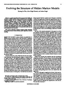
4. Application to Old Faithful Geyser data Geysers are volcanic phenomena whose activity is based on intermittent eruptions of hot and mineralized water. Thus geysers are intermittent thermal springs, from which the water gushes forth by violent jets alternate to break periods. We consider the series of the duration of the eruptions, in minutes, of the Old Faithful Geyser in Yellowstone National Park, Wyoming, USA, recorded from August 1st until August 8th, 1978 (Silverman (1986)). The series presents no missing observation, but we artificially put them in: it is not a strangeness that there are some missing observations in a geyser eruptions series, e.g. Azzalini and Bowman
174 (1990) (we could not analyse that series because the number of missing observations is too high). We chose three isolated missing observations, at time t = 20, 52, 78 and eight missing observations gathered in two separated blocks of three (at time t = 34, 35, 36) and five (from time t = 90 to time t = 94) values. The series is plotted in Figure 1, in which the presence of two hidden states, representing two different levels of the volcanic activity, is evident. The presence of two hidden states, noticing a two-peaks distribution, is confirmed by the continuous approximation of the histogram plotted in Figure 2. The iterative procedure for the identification of the parameters of GHMMs, introduced in Section 3, has been implemented in a GAUSS code. As we have already observed, the choice of the starting values is a matter of primary importance to identify the global maximum, given that the log-likelihood surface for HMMs is often irregular and characterized by many local maxima. Therefore the code repeats more than once the iterative procedure, starting from several different points, randomly chosen in the parameter space � and we compare the stationary points obtained at each run, choosing that with the largest loglikelihood value. Furthermore δ has been assumed known and fixed for any iteration of the EM algorithm, given that the initial distribution is non-informative about the transition probabilities. The variance-covariance matrix of the parameters estimates are obtained from the inverse of a numerical approximation of the Hessian matrix with reverse sign. To estimate the dimension m of the state-space of the Markov chain, according to Leroux and Puterman (1992), we use the Akaike Information Criterion (AIC) and the Bayesian Information Criterion (BIC): we search for that special value m ∗ which maximizes the differ(m) ence ln L (m) T (φ) − am,T , where ln L T (φ) is the log-likelihood function maximized over a HMM with an m-state Markov chain, while am,T is the penalty term depending on the number of states m and the length T of the observed sequence. If am,T = dm , where dm is the dimension of the model, that of the parameters estimated with the � is the number � EM algorithm i.e. m 2 + m , we have the AIC; if am,T = (ln T )dm /2, we have the BIC. In the series of the duration of geyser eruptions, y1 , . . . , y107 , the values y20 , y34 − y36 , y52 , y78 , y90 − y94 have been dropped out of the
175
Fig. 1. Series of the duration of the eruptions of the Old Faithful Geyser, from 1.8 to 8.8 1978
Fig. 2. Continuous approximation of the histogram of the data plotted in Fig. 1
sample; so, as we saw in Subsection 2.1, we have to consider the wstep transition probabilities γi19 ,i21 (2), γi33 ,i37 (4), γi51 ,i53 (2), γi77 ,i79 (2), γi89 ,i95 (6). According to (4), the likelihood function of the observed
176 data, is L 107 (φ) = δ �
� 19 �
�
�
Gt �
t=1
�
·�
77 �
33 �
�
�
G t �3
t=21
�
Gt �
t=53
�
51 �
�
Gt ·
t=37
89 �
�
G t �5
� 107 �
t=79
�
G t 1(m) .
t=95
In the same way, the w-step transition probabilities will be adopted (k+1) to obtain the explicit formulae of the estimators γi,(k+1) , µi(k+1) , σi2 j replacing in vectors Ai,(k)j , Bi(k) , Ci(k) , in expressions (5), (6), (7), the (k) (k) (k) (k) (k) (k) (k) matrices F20 , F34 −F36 , F52 , F78 , F90 −F94 with the identity matrix
(k) (k) (k) and, for any other t, Ft =diag f (yt | 1), f (yt | 2),. . ., f (k) (yt | m) . Performing the EM algorithm for a range of values of the number of states of the Markov chain (m = 1, . . . , 4), we obtain the following maximized values of the log-likelihood and the corresponding AIC and BIC: m
log-likelihood
AIC
BIC
1 2 3 4
−142.62739 −125.91443 −125.91442 −125.91443
−144.62739 −131.91443 −137.91442 −145.91443
−147.3002 −139.9329 −153.9514 −172.6427
Considering both the AIC and the BIC as model selection criteria, we choose a 2-states Markov chain. The sequence of the log-likelihood � � (k) � � � ln L 107 φ converges at the 41th iteration to ln L 107 φ (41) = −125.91443; the estimates of the parameters (standard errors in brackets) of the 2 Gaussian pdfs are
i
1
2
(41)
1.6263
3.4786
2(41)
(0.0000) 0.0470
(0.0000) 0.5546
(0.0000)
(0.0000)
µi σi
177 The estimate of the transition probabilities matrix of the Markov chain (standard errors in brackets) is
� (41)
0 (0.0077) = 0.2318 (0.1038)
1 (0.0077) 0.7682 (0.1038)
from which we have the estimate of the stationary initial distribution δ (41) = (0.1882; 0.8118)� . From the diagonal entries of the transition probabilities matrix, it is also possible to compute the time spent in state i of the Markov chain upon � each �return to it, which has a geometric distribution with mean 1/ 1 − γi,i ; hence the mean number of consecutive eruptions occuring in state i is i
1
2
eruptions
1
4.3144
Observing Figure 1, it is possible to see that no eruption in the low level is followed by another eruption in the same level; for this reason we have γ1,1 = 0 and so 1 is the mean number of consecutive eruptions in state 1.
5. Conclusions In this paper special hidden Markov models (HMMs) {Yt ; X t } used to study univariate non-linear time series have been introduced. They are called Gaussian hidden Markov models (GHMMs), because every observed variable Yt , given a special state i of the Markov chain at time t, is a Gaussian random variable with unknown parameters µi and σi2 . The attention has been focused on the estimation of the parameters δi , γi, j , µi , σi2 , for any state i, j of the Markov chain state-space, when missing observations occur. The estimators of γi, j , µi , σi2 have been obtained by the maximum likelihood method performing the EM algorithm, while the estimators of δi have been obtained by means of the equality δ � = δ � �. We could solve the M step exactly, without using a numerical maximization algorithm, such as the Newton-Raphson
178 method and obtain the explicit formulae of the estimators of the parameters. Hence the procedure is more stable and converges faster in the neighborhood of the maximum. Furthermore an application of GHMMs to geyser data have been shown and the estimates of the parameters of the model computed. In this application, the dimension m of the Markov chain state-space has been estimated by two maximum penalized likelihood methods, the Akaike Information Criterion (AIC) and the Bayes Information Criterion (BIC).
Acknowledgments The authors would like to thanks the referee for his very constructive comments. This research has been supported by the Italian Ministry of University and Scientific Research (MURST) 2000 Grant “Statistics in Environmental Risk Evaluation”.
REFERENCES Albert, P.S. (1991) A Two-State Markov Mixture Model for a Time Series of Epileptic Seizure Counts, Biometrics, 47, 1371-1381. Azzalini, A. and Bowman, A.W. (1990) A Look at Some Data on the Old Faithful Geyser, Applied Statistics, 39, 357-365. Basawa, I.V. and Prakasa Rao, B.L.S. (1980) Statistical Inference for Stochastic Processes, Academic Press, London. Baum, L.E., Petrie, T., Soules, G., and Weiss, N. (1970) A maximization technique occuring in the statistical analysis of probabilistic functions of Markov chains, The Annals of Mathematical Statistics, 41, 164-171. Bickel, P.J., Ritov, Y., and Ryd´en, T. (1998) Asymptotic normality of the maximumlikelihood estimator for general hidden Markov models, The Annals of Statistics, 26, 1614-1635. Dempster, A.P., Laird, N.M., and Rubin, D.B. (1977) Maximum likelihood from incomplete data via the EM algorithm (with Discussion), Journal of the Royal Statistical Society, Series B, 39, 1-38. Elliott, R.J., Aggoun, L., and Moore, J.B. (1995) Hidden Markov Models: Estimation and Control, Springer, New York. Fredkin, D.R. and Rice, J.A. (1992) Maximum likelihood estimation and identification directly from single-channel recordings, Proceedings of the Royal Society of London, Series B, 249, 125-132. Juang, B.H. and Rabiner, L.R. (1991) Hidden Markov Models for Speech Recognition, Technometrics, 33, 251-272.
179 Leroux, B.G. (1992) Maximum-likelihood estimation for hidden Markov models, Stochastic Processes and their Applications, 40, 127-143. Leroux, B.G. and Puterman, M.L. (1992) Maximum-Penalized-Likelihood Estimation for Independent and Markov-Dependent Mixture Models, Biometrics, 48, 545558. MacDonald, I.L. and Zucchini, W. (1997) Hidden Markov and Other Models for Discrete-valued Time Series, Chapman & Hall, London. McLachlan, G.J. and Krishnan, T. (1997) The EM algorithm and extensions, John Wiley & Sons, New York. Silverman, B.W. (1986) Density Estimation for Statistics and Data Analysis, Chapman & Hall, London. Wu, C.F.J. (1983) On the Convergence Properties of the EM Algorithm, The Annals of Statistics, 11, 95-103. Parameter estimation of Gaussian hidden Markov models when missing observations occur Summary We examine hidden Markov models in which the probability density function of every observed variable, given a state of the Markov chain, is Gaussian. The aim of this paper is to show a methodology to obtain the maximum likelihood estimators of the parameters of this class of models that can be computed also when the time series contains missing observations. Our methodology, based on the EM algorithm, is explained analysing a time series about the duration of geyser eruptions.
Stima dei parametri di un modello markoviano latente gaussiano con osservazioni mancanti Riassunto In questo lavoro si considerano quei particolari modelli markoviani latenti in cui la funzione di densit`a di probabilit`a di ogni variabile osservata, dato lo stato della catena di Markov, e` gaussiana. Si vuole qui mostrare una metodologia per ottenere gli stimatori di massima verosimiglianza dei parametri di questa classe di modelli che sia valida anche nel caso in cui la successione di osservazioni sia incompleta. Questa metodologia, che si basa sull’algoritmo EM, e` illustrata attraverso l’analisi di una serie storica relativa alla durata delle eruzioni di un geyser.
Key words Discrete-time stochastic processes; Markov chains; Maximum likelihood estimators; EM algorithm; Geyser data.
[Manuscript received March 2002; final version received June 2002.]