INTRODUCTION TO THE DESIGN AND ANALYSIS OF. ALGORITHMS - Anany
Levitin (Pearson International) Clear and well written and about the right level.
COMP1004: Analysis of Algorithms This part of the course deals with assessing the time-demand of algorithmic procedures with the aim, where possible, of finding efficient solutions to problems. We will not be considering issues related to demands on memory space; for those interested, these are dealt with for example one or other of the references below.
Background reading The material in these books is supplementary to the notes – the books are not essential for this part of the 1004 course. ALGORITHMICS: The Spirit of Computing - David Harel (Addison Wesley) A very readable introduction to the subject, covering most of the areas dealt with in these lectures and also many further topics (some relating to later modules such as COMP3004) – highly recommended. INTRODUCTION TO THE DESIGN AND ANALYSIS OF ALGORITHMS - Anany Levitin (Pearson International) Clear and well written and about the right level. This course doesn't follow the book closely but uses a similar style of pseudocode and some of its examples. ALGORITHMS: Theory and Practice - Giles Brassard and Paul Bratley (Prentice-Hall) Detailed mathematical treatment, goes much further than this course – recommended if you find the material interesting and want to learn more.
COMP1004: Part 2.1
1
1. INTRODUCTION
What is an algorithm? An algorithm is a procedure composed of a sequence of welldefined steps, specified either in a natural language (a recipe can be regarded as an algorithm), or in appropriate code or pseudocode. In these lectures algorithms will be presented in a simplified pseudocode. An algorithm is able to take a ‘legal’ input – eg for multiplication a pair of numbers is legal, but a pair of text files is not – carry out the specified sequence of steps, and deliver an output. Algorithms are procedural solutions to problems. Problems to which algorithmic solutions may be sought fall into four basic classes: • Those that admit solutions that run in ‘reasonable time’ – the class of tractable problems (eg sorting and searching). • Those that probably don’t have reasonable-time algorithmic solutions (eg the Travelling Salesman problem). • Those that definitely don’t have such solutions (eg the Towers of Hanoi). • Those that can’t be solved algorithmically at all – the class of non-computable problems (eg the halting problem). The last three of these will be the subject of later courses; this course will deal mainly with methods for evaluating the timecomplexity of ‘reasonable time’ algorithms, for those tractable problems which do admit such solutions.
COMP1004: Part 2.1
2
A tractable problem may however also have an algorithmic solution which does not have reasonable time demands. Often such an algorithm comes directly from the definition of the problem – a ‘naïve’ algorithm – but a more subtle approach will yield a more practically useful solution. Here’s an example of a problem which is tractable, but which has also has a naive algorithm that has a very fast growing timedemand that makes this algorithm useless for all but very small input instances. Example: evaluating determinants A determinant is a number that can be associated with a square matrix, used for example in the calculation of the inverse of a matrix (you will learn about matrices in the MATH6301 Discrete Mathematics course this term). It has a recursive definition such that det(M), for an nxn (n rows and n columns) matrix, is a weighted sum of n determinants of (n-1)x(n-1) sub-matrices. These in turn can be expressed as the weighted sums of the determinants of (n-1) determinants of (n-2)x(n-2) matrices, and so on. n
det(M) = " (!1) j+1a1j det(M(n) [1, j]), n>1 j=1
= a11, n=1 ( M(n) [i, j] is the (n-1)×(n-1) matrix formed by deleting the ith row and jth column of the n×n matrix M.) This definition can be used as the basis for a simple algorithm, referred to here as the ‘recursive algorithm’. Using it for example for a 3x3 matrix is easy; the calculation takes only a few minutes. For a 4x4 or 5x5 it begins to get messy and time-consuming...
COMP1004: Part 2.1
3
...but for a 10x10 matrix, forget it. Unless you are exceptionally patient you would not want to do this by hand. And even using a computer it takes a significant amount of time. What isn't immediately apparent from the 'to calculate the quantity for an instance of size n, calculate it for n instances of sizes n-1' recursive definition is how much work this implies. The recursive algorithm takes a time in the order of n!, written O(n!), where n! = n×(n-1)×(n-2)...×3×2×1 (later in the course we will show this). ('In O(...)' means 'roughly like (...)' at an intuitive level – later we will formalise the definition.) n! is an extremely fast-growing function, making it unfeasible to use the recursive algorithm for all but very small matrices (n ≤ 5). However there is an alternative algorithm for evaluating a determinant, based on Gaussian elimination, that only takes time in O(n3). The difference between the time-demand of the two algorithms as the input size grows is startling: size of matrix
recursive algorithm
5x5 10 x 10 20 x 20 100 x 100
20 secs 10 minutes >10 million years !!
COMP1004: Part 2.1
Gaussian elimination
0.01 secs 5.5 secs
4
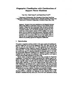
Two ways to approach analysis of algorithms: Empirical: repeatedly run algorithm with different inputs – get some idea of behaviour on different sizes of input → can we be sure we have tested the algorithm on a sufficiently wide range of inputs? → this consumes the very resource (time) we are trying to conserve! Theoretical: analysis of a ‘paper’ version of the algorithm → can deal with all cases (even impractically large input instances) → machine-independent The aim is to obtain some measure of how the time demand of an algorithm grows with the size of its inputs, and to express the result in a simplified way, using order notation, so that the implications can be more easily visualized. Time complexity function
Problem size n 10
102
103
104
log2n
3.3
6.6
10
13.3
n
10
100
103
104
n log2n
33
700
104
1.3x10⁵
n2
100
104
106
108
n3
1000
106
109
1012
2n
1024
1.3x1030
>10100
>10100
n!
3x10⁶
>10100
>10100
>10100
COMP1004: Part 2.1
5
Measuring ‘size of an instance’ Formally, the size |x| of an input instance x is the number of bits needed to encode it, using some easily-decoded format. e.g. for multiplying 2 numbers x & y 010| 100 x
x=2, y=4
y
smaller number padded with leading zeros ‘Size of input’ = 2 x max ( 1+ !"log2 x #$, 1+ !"log2 y#$ ) [ We will use the functions ceiling(x) = !"x #$ = smallest integer ≥ x , floor(x) = !"x #$ = largest integer ≤ x ] But normally a much more informal definition is used which depends on the context, eg problem sorting
‘size of an input instance’ number of items to be sorted
calculating a determinant
number of rows and columns in matrix
finding a minimal spanning tree
number of nodes in the graph
COMP1004: Part 2.1
6
Measuring ‘time taken’ The objective is to make the time-cost analysis machineindependent. The difference between running the same algorithm on two different machines is only going to be some constant factor (eg. “this machine is twice as fast as that one”) which is the same for all input sizes. The kind of difference that really counts is the sort that itself increases with size – the difference between n log n and n2, or between n3 and n!. A machine-independent measure of time is given by counting elementary operations. These are simple operations used as primitives by all the candidate algorithms – for example when we say that the cost of a sorting algorithm “grows like n2” we will usually be counting the number of comparisons done as a function of n, the number of things to be sorted. Other operations that can be used as ‘elementary’ time-counters are Boolean operations (AND, OR, etc.), assignments, and mathematical operations such as addition, subtraction, multiplication and division. Elementary operations are considered to themselves be of negligible cost, and are sometimes – for simplicity – referred to as being of ‘unit cost’ or taking ‘unit time’. Note: operations which are ‘primitive’ and considered to be of trivial intrinsic cost – so that they can be used as time-counters – in some contexts may not be so lightly dismissed in others. (For example multiplying 2 numbers can almost always be thought of as an elementary operation, but there are some applications, such as cryptology, using very large numbers (100s or 1000s of decimal digits), where the cost of multiplication is not trivial! Then multiplication itself needs to be broken down into simpler operations (single-bit ones) and better algorithms (like Strassen’s algorithm – see later) looked for.)
COMP1004: Part 2.1
7
Forms of time-complexity analysis Worst case This is the easiest form of analysis and provides an upper bound on the efficiency of an algorithm (appropriate when it is necessary to ensure a system will respond fast enough under all possible circumstances- eg. controlling a nuclear power plant) Average case There may be situations where we are prepared to put up with bad performance on a small proportion of inputs if the ‘average performance’ is favourable. What does ‘average performance’ mean? Either sum the times required for every instance of a particular size, divide by the number of instances, or evaluate performance with respect to an ‘average instance’. (For a sorting algorithm this might well be a randomly ordered file- but what is an average instance for a program processing English-language text?) Average case analysis is mathematically much more difficultmany algorithms exist for which no such analysis has been possible. Best case This kind of analysis differs from the other two in that we consider not the algorithm but the problem itself. It should really be referred to as ‘best worst case’ analysis, because we aim to arrive at bounds on the performance of all possible algorithmic solutions, assuming their worst cases. Best case analysis is based on an consideration of the logical demands of the problem at hand – what is the very minimum that any algorithm to solve this problem would need to do, in the worst case, for an input of size n?
COMP1004: Part 2.1
8
Example: Consider the multiplication of two n-bit numbers. Any algorithm to solve this problem must at least look at each bit of each number, in the worst case – since otherwise we would be assuming that the product could in general be independent of some of the 2n bits – and so we can conclude that multiplication is bounded below by a linear function of n.
Order Notation The result of a time-complexity analysis may be some long and complicated function which describes the way that time-demand grows with input size. What we really want to know is how, roughly, these time-demand functions behave – like n? log n? n3? The objective of using order notation is to simplify results of complexity analysis so that the overall shape – and in particular, the behaviour as n → ∞ (asymptotic behaviour) – of the timedemand functions are more clearly apparent.
O-notation ‘O’ can provide an upper bound to time-demand in either worst or average cases. Intuitively, ‘f(x) is O(g(x))’ means that f(x) grows no faster than g(x) as x gets larger. Formally, The positive-valued function f(x) ∈ O(g(x)) if and only if there is a value x0 and a constant c>0 such that
for all x ! x 0 ,
f(x) " c.g(x)
(Note: the restriction in the definition here – for simplicity – that f(x) be ‘positive-valued’ isn’t likely to cause problems in algorithmic applications since functions will represent ‘work done’ and so will always return positive values in practice.)
COMP1004: Part 2.1
9
Useful properties of ‘O’ 1. O( k.f(n) ) = O( f(n) ), for any constant k This is because multiplication by a constant just corresponds to a re-adjustment of the value of the arbitrary constant ‘k’ in the definition of ‘O’. This means that under O-notation, we can forget constant factors (though these ‘hidden constants’ might be important in practice, the don’t change the order of the result). Note that as a consequence of this, since loga n = loga b× logb n there is no effective difference between logarithmic bases under O-notation; conventionally we just use O(log n), forgetting the (irrelevant) base.
COMP1004: Part 2.1
10
2. O( f(n) + g(n) ) = O( max( f(n),g(n) ) ) (for those interested the proof is on p.56 of Levitin)
‘max’ here is a shorthand way of saying ‘the part that grows the fastest as n → ∞ ’. This result enables us to simplify the result of a complexity analysis, for example
n3 + 3n2 + n + 8 ∈ O(n3 + (3n2 + n + 8)) = O(max(n3 ,3n2 + n + 8)) = O(n3 )
3. O( f(n) ) U O( g(n) ) = O( f(n) + g(n) ) (not so easy to prove!)
= O( max(f(n),g(n)) ), by 2. above. This last means that where an algorithm consists of a sequence of procedures, of different time-complexities, the overall complexity is just that of the most time-demanding part.
Examples of proofs using O-notation [Note: You can assume in all such proofs that n>0, as in this course n will represent ‘size of an input’.] For example, is it true that (i) n 2 ∈ O(n3 ) ? (ii) n3 ∈ O(n 2 ) ? The general way to proceed is as follows: • Assume the assertion is true. • Work from the definition of ‘O’, and try to find suitable values of c and no • If you can find any pair of values (there’s no unique pair) the assertion is, in fact, true. If there is some fundamental reason why no pair c,n0 could be found, then the original hypothesis was wrong and the assertion is false.
COMP1004: Part 2.1
11
( i) Is n2 ∈ O(n3 ) ? Assume it is. Then
n2 ! cn3 " 0, $ n2 (1! cn) " 0, $ cn # 1, 1 $ n# , c
for all n # n0 for all n # n0 for all n # n0 for all n # n0
Choosing (for example) c=2, n0=1 is satisfactory and so it’s TRUE that n 2 ∈ O(n3 ) .
(ii) Is n3 ∈ O(n2 ) ? Again, assume it is. Then
n3 ! cn2 " 0, for all n # n0 $ n2 (n ! c) " 0, for all n # n0 $ n ! c " 0, for all n # n0 But c has to have a fixed value. There is no way to satisfy n≤c, for all n ≥ n0 for a fixed c. Hence the original assumption was FALSE, and n3 ∉ O(n 2 ) . Notes • When answering the question ‘Is f (n) ∈ O(g(n)) ?’ it is not sufficient to draw a picture showing the curves f(n) and g(n) -- that can illustrate your argument, but isn’t in itself a proof, as the question is about what happens as n → ∞ , so can’t be resolved by looking at any finite range of n. • If you are asked to base a proof on 'the formal definition of O-notation' don't base your argument on the three properties listed on pp.10-11. Argue from the definition of O-notation, as above.
COMP1004: Part 2.1
12
Hierarchies of complexity Let n be the ‘size’ of an input instance, in the usual informal definition (eg degree of a polynomial, length of a file to be sorted or searched, number of nodes in a graph). Complexity O(1) Constant time: all instructions are executed a fixed number of times, regardless of the size of the input. Example: taking the head of a list. O(log n) Logarithmic: program gets only slightly slower as n grows (typically by using some transformation that progressively cuts down the size of the problem). Example: binary search. O(n) Linear: a constant amount of processing is done on each input element. Example: searching an unordered list. O(n log n) Typical of ‘divide and conquer’ algorithms, where the problem is solved by breaking it up into smaller subproblems, solving them independently, then combining the solutions. Example: quicksort. k Polynomial: most often arises from the presence of k O(n ) nested loops (examples: insertionsort (k=2); Gaussian elimination method for a calculating a determinant (k=3). n Exponential: very fast-growing (assuming a>1), O(a ) essentially unusable for all but very small instances. Example: Towers of Hanoi (a=2). Factorial: even worse! Example: recursive evaluation O(n! ) of a determinant. Only algorithms running in polynomial time (those which are in O(nk ) for some k) are effectively usable; only problems which admit such algorithms are effectively soluble (tractable). Thus finding a determinant is soluble in reasonable time because it has a ‘good’ algorithm running in O(n3 ) as well as an unusable O(n!) one, but the Towers of Hanoi puzzle isn’t, because it can be demonstrated that there are no ‘good’ algorithms possible in this case. (More about such intractable problems in the 3rd year COMP3004 Computational Complexity course.)
COMP1004: Part 2.1
13
2. ANALYSIS OF NONRECURSIVE ALGORITHMS There is not a clear set of rules by which algorithms can be analysed. There are, however, a number of techniques which appear again and again. The best way to learn about these is really though examples. Algorithms consist of sequences of procedural steps which may themselves involve loops of fixed (‘for...’) or indeterminate (‘while…’, etc) length, or of recursive function calls (see later).
We will start with the simplest cases: SEQUENTIAL OPERATIONS
Step i – O( f(n) ) Step (i+1) – O( g(n) ) The combination of the ith and (i+1)st steps takes a time in O( f(n) ) U O( g(n) ). Use
O( f(n) ) U O( g(n) ) = O( max( f(n),g(n) ) ) to justify neglecting all but the most time-costly step.
COMP1004: Part 2.1
14
Example: multiplication (i) Shift-and-add multiplication ("long multiplication") 1.….....01 x 1…...…11 ………...1 …………0 …………00
n bits in each number
+ + … +…….00……..0
n partial values longest is 2n-1 bits result is 2n bits in worst case
(1) Compute n partial values, each requiring n single-bit multiplications (2) Add the partial values (estimate as (n-1) additions of pairs of (2n-1)-bit numbers (upper bound)) Complexity (single-bit operations) Step(1) n2 Step(2) (2n-1)(n-1) = 2n2−3n+1 Total 3n2 - 3n+1 ∈ O(n2) n=5 example
0 0 0 0 0 0 0 0 0 0 0 0 0 0 0
0 0 0 1 0 0 0 1 0 0 1 0 1 0 1
0 0 0 0 0 0 0 0 0 0 0 0 1 0 1
× 0 1 0 0 0 1 0 0 0 1 0 0 0 0 0
1 0 1 0 0 1 0 1 0 1 0 1 1 0 1 0 1
0 1 0 0 0 1 0 1 0 1 0 1 1 0 0 0 0
0 0 0 1 0 0 0 0 0 0 0 0 0 0 0 0 0
1 1 1 1 0 0 0 0 0 0 0 0 0 0 0 0 0
1 1 1 0 0 0 0 1 0 0 0 1 0 0 1 0 1
(19) (11) 5x5=25 single bit multiplications having added top two rows (9 additions)
having added top two rows (9 additions) having added top two rows (9 additions) having added top two rows (9 additions)
Total number of single bit operations = 25 + 9 + 9 + 9 + 9 = 61 (= 3x52-3x5+1) Ans = 011010001 = 0x256+1x128+1x64+0x32+1x16+0x8+0x4+0x2+1x1 = 209
COMP1004: Part 2.1
15
(ii) A la russe method The idea is to start with two columns (where ‘/’ in the first column means integer division, ie dropping the remainder): a a/2 a/4 i i 1
×
b 2b 4b i i i
Create a third column, containing a copy of the number from the second column everywhere the number in the first column is odd. Add up this third column to get the result. eg
19 9 4 2 1
× 11 × 22 × 44 × 88 × 176
11 +22 +176 =209
There are O(n) entries in the columns, each involving work O(1), since each entry is made by either a right-shift (left column) or by adding a zero (right column). Adding the third column is O(n2). So ‘à la russe’ is also O(n2) overall – but it’s slightly faster than shift-and-add multiplication because it is still only O(n) before the addition stage. Lower bound on the time-complexity of multiplication We argued earlier that every algorithm for multiplying two n-bit numbers will require at least 2n single-bit operations, so has a best worst case in O(n). There is thus scope for algorithms whose performance improves on that of the simple O(n2) ones above and has a worst-case performance somewhere in between O(n) and O(n2) – we will see one such algorithm later, Strassen’s algorithm, which has a worst-case performance in O(n1.59... ).
COMP1004: Part 2.1
16
Sums of series Before moving on to look at algorithms with loops and recursion, we need to know how to evaluate sums of series.
Arithmetic series The notation b
∑ f (i) i=a
means f(a)+f(a+1)+……+f(b). Note we can use the notation even when f is independent of i: b
! c means (c+c+…+c) = c(b-a+1) i=a
!!!
b-a+1 times
The simplest – and most useful – case is when f(i) = i. In this case it is easy to derive a formula (a ‘closed form’ which does not have the summation symbol) for
b
∑ f (i): i=a
2×
n
∑ i= i =1
1 + 2
+ … + (n-1) + n
+ n + (n-1) + … +
2
+1
=(n+1)+ (n+1)+ … + (n+1)+(n+1) n copies = n(n+1) n
→
n
∑ i = 2 (n + 1) i =1
COMP1004: Part 2.1
17
It’s sometimes the case that the sum to be evaluated doesn’t start with i=1: n
n
i= j
i =1
∑ i= ∑ i -
j −1
∑i i =1
n ( j − 1) = (n + 1) j 2 2
Geometric series This is the other type of simple series summation which is very useful in algorithmics. Let →
S(n) = a + a2+ a3+…+ an = 2
3
4
a.S(n) = a + a + a +…+ a = S(n) – a + an+1
n+1
n
∑a
i
i=1
So
a(1 − a n ) a= ∑ 1− a i=1 n
i
for a ≠ 1
Note that the formula works only for a ≠ 1 - if a=1 get sum 0/0, which gives an undefined value. The calculation has to be done differently in this case: If a = 1: n
n
∑ a = ∑ 1 = (1 + 1+ …+1) = n i=1
i
i=1
COMP1004: Part 2.1
n terms
18
Estimating a sum by an integral In real-life algorithmic analyses it’s often the case that the series to be summed is not of one of the above simple forms, or any other for which a sum formula can be easily found. (The average-case analysis of Quicksort – considered later – is an example of this sort.) It’s then necessary to estimate the sum. Assume that where a sum from a..b is required that the function f(x) is non-decreasing between x=a and x=b+1.
The area in the boxes (where in the example a=1, b=4) is the 4
desired sum ∑ f (i) . i =1
It can be seen from the illustration that this area is not greater than the area under the curve from x=1 to x=5. In general using this graphical argument b
# f(i) i=a
COMP1004: Part 2.1
b+1
!
" f(x) dx a
19
It can also be shown that if the function f(x) is non-increasing between x=a-1 and x=b that b
b
$ f(i)
!
# f(x) dx
a"1
i=a
Draw a similar picture and think about it. (If you think this variant of the approximation is less relevant because algorithmic work functions are not expected to be uniformly decreasing, consider that components of them might still behave this way -- see Gaussian elimination example later.)
Example: Use
n
∑ i2
n
∑ i2
i =1 n +1
∫x
≤
i =1
=? 2
dx
1
n+1
=
! x3 $ #" 3 &%
1
=
1
3 ! $ n +1 - 1& , and hence 3# " %
(
)
n
∑ i2
∈ O(n3 )
i =1
(A more general argument along the same lines can be used to show that
n
∑ ik
∈ O(nk +1 ) )
i =1
COMP1004: Part 2.1
20
ALGORITHMS WITH LOOPS In the simplest cases where the loop is executed a fixed number of times (a ‘for’ loop) the complexity is just the cost of one pass through the loop multiplied by the number of iterations. ALGORITHM Sum( A[0..n-1] ) // Outputs the sum of the elements in A[0..n-1] sum