Nov 14, 2014 - centers spatially related to annotated semantic parts or bounding boxes. This allows us not just ... ing. The code is available at http://www.inf-cv.uni-jena.de/part_ ..... channel instead of one call for each element of the channel.
Part Detector Discovery in Deep Convolutional Neural Networks
arXiv:1411.3159v2 [cs.CV] 14 Nov 2014
Marcel Simon, Erik Rodner, and Joachim Denzler Computer Vision Group, Friedrich Schiller University of Jena, Germany www.inf-cv.uni-jena.de
Abstract. Current fine-grained classification approaches often rely on a robust localization of object parts to extract localized feature representations suitable for discrimination. However, part localization is a challenging task due to the large variation of appearance and pose. In this paper, we show how pre-trained convolutional neural networks can be used for robust and efficient object part discovery and localization without the necessity to actually train the network on the current dataset. Our approach called “part detector discovery” (PDD) is based on analyzing the gradient maps of the network outputs and finding activation centers spatially related to annotated semantic parts or bounding boxes. This allows us not just to obtain excellent performance on the CUB2002011 dataset, but in contrast to previous approaches also to perform detection and bird classification jointly without requiring a given bounding box annotation during testing and ground-truth parts during training. The code is available at http://www.inf-cv.uni-jena.de/part_ discovery and https://github.com/cvjena/PartDetectorDisovery.
1
Introduction
In recent years, the concept of deep learning has gained tremendous interest in the vision community. One of the key ideas is to jointly learn a model for the whole classification pipeline from an input image to the final outputs. A successful model especially for classification are deep convolutional neural networks (CNN) [1]. A CNN model can be seen as the concatenation of several processing steps similar to algorithmic steps in previous “non-deep” recognition models. The steps sequentially transform the given input into a likely more abstract representation [2,3,4] and finally to the expected output. Due to the large number of free parameters, deep models usually need to be learned from large-scale data, such as the ImageNet dataset used in [1], and learning is a computationally demanding step. The very recent work of [5,6,7] shows that pre-trained deep models can also be exploited for datasets which they have not been trained on. In particular, efficient and very powerful feature representations can be obtained that lead to a significant performance improvement on several vision benchmarks. Our work follows a similar line of thought and in particular the question we were interested in is: “Can we re-use pre-trained deep convolutional networks for part discovery and detection? Does a deep model
Compute gradients with respect to positions
Part discovery by comparing with ground-truth
Select channel with smallest distance to ground-truth
Testing
Marcel Simon, Erik Rodner, Joachim Denzler
0.1
0.3 gradient maps for channels
CNN head detector
0.7
pre-learned CNN
Channel most corresponding to ground-truth part
Part discovery and learning
2
ground-truth head position
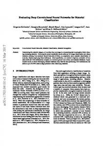
Fig. 1. Outline of our approach during learning using the part strategy: (1) compute gradients of CNN channels with respect to image positions, (2) estimate activation centers, (3) find spatially related semantic parts to select useful channels that act as part detectors later on. learned on ImageNet already include implicit detectors related to common parts found in fine-grained recognition tasks?” The answer to both questions is yes and to show this we present a novel part discovery and detection scheme using pre-trained deep convolution neural networks. Object representations for visual recognition are often part-based [8,9] and in several cases information about semantic parts is given. The parts of a bird, for example, include the belly, the wings, the beak and the tail. The benefit of part-based representations is especially notable in fine-grained classification tasks, in which the objects of different categories are similar in shape and general appearance, but differ greatly in some small parts. This is also the application scenario considered in our paper. Our technique for providing such a part-based representation is based on computing gradient maps with respect to certain channel outputs and finding clusters of high activation within. This is followed by selecting channels which have their corresponding clusters closest to ground-truth positions of semantic parts or bounding boxes. An outline of our approach is given in Fig. 1. The most interesting aspect is that after finding these associations, parts can be reliably detected without much additional computational effort from the results of the deep CNN.
2
Related Work
CNN for Classification The approach of Krizhevsky et al. [1] demonstrates the capabilities of multilayered architectures for image classification by achieving
Part Detector Discovery in Deep Convolutional Neural Networks
3
an outstanding error rate on the LSVRC2012 dataset. Donahue et al. [5] use a CNN with a similar architecture and analyze how well a network trained on ImageNet performs on other not related image classification datasets. They use the output of a hidden layer as feature representation followed by a SVM [10] learned on the new dataset. The authors have also published “DeCAF”, an open source framework for CNNs [5], which we also use in our work. Similar studies have been done by [6,7]. In contrast to their work, we focus on part discovery with pre-trained CNNs rather than classification. An important aspect of [4] is the qualitative analysis of the learned intermediate representations. In particular, they show that CNNs trained on ImageNet contain models for basic object shapes at lower layers and object part models at higher layers. This is exactly the property that we make use of in our approach. Although the CNN we use was not particularly trained on the fine-grained task we consider, it can be used for basic shape and part detection. CNN for Object Detection Motivated by the good results of CNNs in classification, several methods were proposed to apply this technique to object detection. Erhan et al. [11] use a deep neural network to directly predict the coordinates of a fixed number of bounding boxes and the corresponding confidence. They determine the category of the object in each bounding box using a second CNN. A main drawback of this approach is the fixed number of bounding box proposals once the network has been trained. In order to change the number of proposals, the whole networks needs to be trained again. An alternative to the direct prediction of the bounding box coordinates is presented in [12]. They train a deep neural network to predict an object mask at multiple scales. While the predicted mask is similar to our gradient maps, they need to train an additional CNN specifically for the object detection task. Simonyan et al. [13] perform object localization by analyzing the gradient of a deep CNN trained for classification. They compute the gradient of the winning class score with respect to the input image. By thresholding the absolute gradient values, seed background and seed foreground pixels are located and used as initialization for the GrabCut segmentation algorithm. We make use of their idea to use gradients. However, while [13] use the gradients for segmentation, we use them for part discovery. In addition to this, we introduce the idea of using intermediate layers and techniques like the aggregation of gradients of the same channel. CNN for Part Localization Many classification approaches in fine-grained recognition use part-based object models and hence also require part detection. At the moment, most part-based models use low-level features like histogram of oriented gradients [14] for detection and description. Examples are the deformable part model (DPM) [8], regionlets [15], and poselets [16]. Facing the success of features from deep CNN, a current line of research is the use of these features as a replacement for the low-level features of the part-based models. For example, [5] relies on deformable part descriptors [17], which is inspired by DPM. While the localization is still done with low-level features, the descriptor is calculated using the activations of a deep CNN for each predicted part.
4
Marcel Simon, Erik Rodner, Joachim Denzler
Zhang et al. [18] use poselets for part discovery as well as detection and calculate features for each region using a deep CNN. While DPM and regionlets work well on many datasets, they face problems on datasets with large intraclass variance and unconstrained settings especially due to the low-level features that are still used for localization. In contrast, our approach implicitly exploits all high-level features that a large CNN has learned already. It also allows us to solve part localization and the consequent classification within the same framework. Entirely replacing the low-level features is difficult, because a CNN produces global features. Zou et al. [19] solves this by associating the output of a hidden layer with spatially related parts of the input. This allows them to apply the regionlets approach. However, their approach requires numerous evaluations of the CNN and the features are not arbitrarily dense. In contrast, our approach is working on the full resolution of the input. The work of Jain et al. [20] uses the sliding window approach for part localization with CNNs. They evaluate a CNN at each position of the window in order to detect human body parts in images without using bounding box annotations. This requires hundreds or thousands of CNN evaluations. As sufficiently large CNNs take some time for prediction, this results in long run times. In contrast, only one forward- and one back-propagation pass per part is required for the localization with our approach. In [21] and [22], the part positions are estimated by a CNN specifically trained for this task. The outputs of their network are the coordinates of each part. In contrast to their work, our approach does not require any separately trained neural network but can exploit a CNN already trained for a different large-scale classification task.
3
Localization with Deep Convolutional Neural Networks
In the following, we briefly review the concept of deep CNNs in Sect. 3.1 and the use of gradient maps for object localization presented by Simonyan et al. [13] in Sect. 3.2 as these are the ideas our work is based on. 3.1
Deep Convolutional Architectures
A key idea of deep learning approaches is that the whole classification pipeline consists of one combined and jointly trained model. Many non-deep systems rely on hand-crafted features and separately trained machine learning algorithms. In contrast, no hand-crafted features are required in deep learning architectures as they are automatically learned from the training data and no separately trained machine learning algorithm is required as the deep architecture also covers this part. Most recent deep learning architectures for vision are based on a single CNN. CNNs are feed forward neural networks, which concatenate several layers of different types. These layers are often related to techniques that a lot of nondeep approaches for visual recognition used without joint parameter tuning: 1. Convolutional layers perform filtering with multiple filter masks, which is related to computing the distance of local features to a given codebook in the common bag-of-words (BoW) pipeline.
Part Detector Discovery in Deep Convolutional Neural Networks
5
Class Scores y dense Input x
Conv 1
Conv 2
Conv 5
FC 1
dense dense FC 3 FC 2
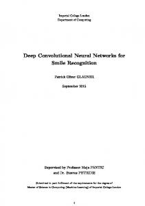
Fig. 2. Example of a convolutional neural network used for classification. Each convolutional layer convolves the output of the previous layer with multiple learned filter masks, applies an element-wise non-linear activation function, and optionally combines the outputs by a pooling operation. The last two layers are fully connected layers and multiply the input with a matrix of learned parameters followed by a non-linear activation function. The output of the network are scores for each of the learned categories. 2. Pooling layers spatially combine filter outputs, which is related to classical spatial pyramid matching [23]. 3. Non-linear layers, such as the rectified linear unit used by [1], are related to non-linear encoding techniques for BoW [24]. 4. Several fully connected layers at the end act as nested linear classifiers. The final output of the CNN are scores for each object category. The architecture is visualized in a simplified manner in Fig. 2. For details about the network structure we refer to [1] and [5] since we use the same pre-trained CNN. As visualized in the figure, we will denote the transformation performed by the CNN as a function fθ (x), which maps the input image x to the classification scores for each category using the parameter vector θ. We omit θ in the following text since it is not relevant for our approach. The function f is a concatenation of functions f(x) = f (n) ◦ f (n−1) ◦ · · · ◦ f (1) (x), where the f (1) , f (2) , . . . , f (n) correspond to the n layers of the network. Furthermore, let g (k) (x) := f (k) ◦ f (k−1) ◦ · · · ◦ f (1) (x) be the output and x(k) := g (k−1) (x) the input of the k-th layer. Please note that f (j) represents only the transformation of layer j, while g (j) includes all transformations from input image to layer j. Furthermore and most importantly for our approach, the output of the first layers is organized in channels with each element in the channel being related to a certain area in the input image. The outputs of a channel are the result of several nested convolutions, non-linear activations and pooling operations applied to the input image. Therefore, we can view them as results of pooled detector scores, a connection that we make use of for our part discovery scheme in Sect. 4. 3.2
Localization Using Gradient Maps
Deep convolutional neural networks trained for classification can also be used for other visual recognition tasks like object localization. Simonyan et al. [13]
6
Marcel Simon, Erik Rodner, Joachim Denzler
Fig. 3. Examples for the gradient gradient maps (continuous and thresholded with the 95%-quantile) that are calculated with respect to the winning class score. present a method, which calculates the gradient of the winning class score with respect to the input image. The intuition is that important foreground pixels have a large influence on the classification score and hence have a large absolute gradient value. Background pixels, however, do not influence the classification result and hence have a small gradient. The experiments in [13] support this intuition and it allows them to use this information for segmentation of foreground and background. The next paragraph briefly reviews the calculation of the gradients as we also use gradient maps in our system. i The calculation of the gradient ∂f ∂x of the model output (f (x))i with respect to the input image x is similar to the back-propagation of the classification error during training. Using the notation introduced in Sect. 3.1, the gradient can be computed using the chain rule as (n)
∂fi ∂g (n−1) ∂fi ∂g (n−1) ∂g (2) ∂g (1) ∂g ∂g (1) = (n−1) (n−2) . . . (1) = i(n) (n−1) . . . . ∂x ∂x ∂x ∂g ∂g ∂g ∂x ∂x
(1)
∂g (j)
Each factor ∂x(j) of this product is a Jacobian matrix of the output g (j) with respect to the input x(j) of layer j . This means that the gradient can be computed layer by layer. These factors are also calculated during back-propagation. The only difference is that the last derivative is with respect to x instead of θ. i The gradient ∂f ∂x can be reshaped such that it has the same shape as the input image. The result is called gradient map and Fig. 3 visualizes the gradient maps that are calculated with respect to the winning class score for two examples. At first glance, a gradient might seem very similar to a saliency map. However, while a saliency map captures objects that distinguish themselves from the background [25], the gradient values are only large for pixels, that influence the classification result. Hence, conspicuous background objects will be highlighted in a salient map but not in a gradient map as they do not influence the score of the winning class. The second image in Fig. 3 is a good example, whose strong background patterns are not highlighted in the gradient map.
4
Part Discovery in CNNs by Correspondence
Recent fine-grained categorization experiments have shown that the location of object parts is a valuable information and allows to boost the classification
Part Detector Discovery in Deep Convolutional Neural Networks
7
accuracy significantly [26,9,5]. However, the precise and fast localization of parts can be a challenging task due to the great variety of poses in some datasets. In Sect. 4.1, we present a novel approach for automatically detecting parts of an object. Given a test image of an object from a previously known set of categories, the algorithm will detect visible parts and locate them in the image. This is followed by Sect. 4.2 presenting a part-based classification approach, which is used as an application of our part localization method in the experiments. 4.1
Part Localization
Gradient Maps for Part Discovery Like the object localization system of the previous section, our algorithm requires a pre-trained CNN trained for image classification. The classification task it was trained for does not need to be directly related to the actual part localization task. For example, we used for our experiments the model of [5], which was trained on the ImageNet dataset. However, all our experiments are performed on the Caltech Birds dataset. The part localization is done by calculating the gradient of the output elements of a hidden layer with respect to the input image. Suppose the selected layer has m output elements, then m gradients with respect to the input image and hence m gradient maps are computed. The calculation of the gradient maps for each element of a hidden layer is done in a similar way as the gradient of a ∂g
(b)
class score. Let b denote the chosen hidden layer. Then, the gradient ∂xj (x) of the j-th element of layer b with respect to the input image x is calculated as (b)
(b)
(b)
∂gj ∂gj ∂g (b−1) ∂gj ∂g (1) ∂g (b−1) ∂g (1) = (b−1) (b−2) . . . = . · . . . ∂x ∂x ∂x ∂g ∂g ∂x(b) ∂x(b−1)
(2)
As before, we can also make use of the back-propagation scheme for gradients already implemented in most CNN toolboxes. The gradient maps of the same channel are added pixelwise in order to obtain one gradient map per channel. The intuition is that each element of a hidden layer is sensitive to a specific pattern in the input image. All elements of the same channel are sensitive to the same pattern but are focused on a different location of this pattern. Part Discovery by Correspondence We now want to identify channels, which are related to object parts. In the following, we assume that the groundtruth part locations zi of the training images xi are given. However, our method can be also provided with the location of the bounding box only as we will show later. We associate a binary latent variable hk with each channel k, which indicates whether the channel is related to an object part. Our part discovery scheme can be motivated as a maximum likelihood estimation of these variables. First, let us consider the task of selecting the most related channel corresponding to a part which can be written as (assuming xi are independent samples): kˆ = argmax1≤k≤K p(X | hk = 1) = argmax 1≤k≤K
N Y p (hk = 1|xi ) p (xi ) . p (hk = 1) i=1
(3)
8
Marcel Simon, Erik Rodner, Joachim Denzler
where X is the training data and K is the total number of channels. In the following, we assume a flat prior for p(hk = 1) and p(xi ). The term p (hk = 1|xi ) expresses the probability that channel k corresponds to the part currently under consideration given a single training example xi . This is the case when the position pki estimated using channel k equals the ground-truth part position zi . However, the estimated position pki is likely not perfect and we assume it to be a Gaussian random variable distributed as pki ∼ N (µki , σ 2 ), where µki is a center of activation extracted from the gradient map of channel k. We therefore have: p(hk = 1|xi ) = p(pki = zi |xi ) = N (zi |µki , σ 2 )
(4)
Putting it all together, we obtain a very simple scheme for selecting a channel: kˆ = argmax
N X
1≤k≤K i=1
log p(hk = 1|xi ) = argmin
N X
1≤k≤K i=1
kµki − zi k2
(5)
For all gradient maps of all training images, the center of activation µki is calculated as explained in the subsequent paragraph. These locations are compared to the ground-truth part locations zi by computing the mean distance. Finally, for each ground-truth part, the channel with the smallest mean distance is selected. The result is a set of channels, which are sensitive to different parts of the object. There does not need to be a one-to-one relationship between parts and channels, because the neural network is not trained on semantic parts. We refer to this method as part strategy. Part Discovery without Ground-truth Parts In many scenarios, groundtruth part annotations are not available. Our approach can also be applied in these cases by selecting relevant channels based on the bounding box of the training images only. We evaluate two different approaches related to different models for p(hk = 1|xi ). First, we count for every channel how often the activation center is within the bounding box BB(xi ) of the image xi . We select the channels with the highest count, as these are most likely to correspond to the object of interest. It can be shown that this counting strategy is related to the following model for arbitrary 0 < � < 1: ( 1 − � µki ∈ BB(xi ) (6) p(hk = 1|xi ) = � otherwise Second, we extend the first approach by taking the distance to the bounding box border into account. If the activation center of a channel is within the bounding box of a training image, the cost is 0. If it is outside, the cost equals to the Euclidean distance to the bounding box border. Finding Activation Centers The assumption for finding the center of activation µi is that high absolute gradient values are concentrated in local areas of the gradient maps and these areas correspond to certain patterns in the image. In order to robustly localize the center point of the largest area, we fit a
Part Detector Discovery in Deep Convolutional Neural Networks Input image
Body
Head
Wings
Input image
Body
Head
9
Wings
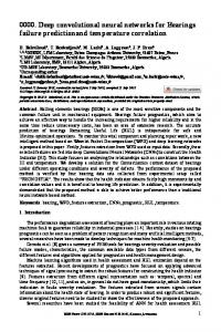
Fig. 4. Examples for gradient maps. Each group of images first shows the input image and then the gradient maps of the channels associated with the body, head and the wings. A light blue to red color means, that the gradient values of the corresponding pixel is high. A deep blue corresponds to a gradient value of zero.
Gaussian mixture model with K components to the pixel locations weighted by the normalized absolute gradient values. We then take the mean location of the most prominent cluster in the mixture as the center of activation. In comparison to simply taking the maximum position in the gradient map, this approach is much more robust to noise as we show in the experiments. Part Detection In order to locate parts in a new image, the gradient maps for all selected channels are calculated. The activation center is estimated and returned as the location of the part. If the gradient map is equal to 0, the part is likely not visible in the image and marked as occluded. Figure 4 visualizes the gradient maps for some test images used in our experiments. For each image, three channels are shown which are associated with semantic parts of a bird. In each group of images, the input is on the left followed by the normalized gradient maps of the channels associated with the body, head and the wings. A light blue to red color corresponds to a large absolute gradient value while a deep blue represents a zero gradient. Why should this work? The results of [4] suggest that at least in the special case of deep CNNs, each element of a hidden layer is sensitive to specific patterns in the image. “Sensitive” means in this case that the occurrence of a pattern leads to a high change of the output. There is an implicit association between certain image patterns and output elements of a layer. In higher layers these patterns are increasingly abstract and hence might correspond to a specific part of an object. Our method automatically identifies channels with this property. As an example, suppose the input of a deep architecture is a RGB color image and the first and only layer is a convolutional layer with two channels representing different local edge filters. If the first filter mask is a horizontal and the second one a vertical edge filter mask, then the first channel is sensitive to horizontal edge patterns and the second one to vertical edge patterns. This example also illustrates that at least in the case of convolutional layers any output element of the same channel reacts to the same pattern and that each
10
Marcel Simon, Erik Rodner, Joachim Denzler
element just focuses on a different area in the input image. Of course, the example only discusses low-level patterns without any direct connection to a specific part. However, experiments [4] indicate that in higher layers the patterns are more complex and correspond, for example, to wheels or an eye. Implementation Details At first, it might seem that simply adding the gradients of all elements of a channel causes a loss of information. Negative and positive gradients can cancel and might cause a close to zero gradient for a discriminative pixel. Possibly adding the absolute gradient values seems to be the better approach, but this is not the case. First, since each element of a channel focuses on a separate area in the input image, the cancellation of positive and negative gradients is negligible. A small set of experiments supports this. Second, calculating the sum of gradients requires only one back-propagation call per channel instead of one call for each element of the channel. In our experiments, each channel has 36 elements. Hence, there is a speedup of 36× in our case. The reason for this is the back-propagation algorithm which directly calculates the sum of gradients if initialized correctly. We have already showed how ∂g
(b)
to calculate the gradient ∂xj of a element with respect to the input image. It is possible to rewrite the calculation such that it shows more clearly how to apply the back-propagation algorithm. Let ej be the j-th unit vector. Then (b)
(b) (b−1) (2) (1) ∂gj ∂gθ ∂g ∂g ∂g ∂g (b) = ej · = ej · (b−1) · θ(b−2) · · · · · θ(1) · θ (x) ∂x ∂x ∂x ∂gθ ∂gθ ∂gθ
(7)
(b)
where ∂g∂x is the Jacobian matrix containing the derivatives of each output element (the rows) with respect to each input component of x (the columns). Here, ej is the initialization for the back-propagation at layer b and all the other factors are applied during the backward pass. In other words, the initialization ej (b)
selects the j-th row of the Jacobian matrix ∂g∂x . Suppose there would be more than one element of ej equal to 1. Then the result is the sum of the corresponding gradient vectors. Let sc = (0, . . . , 0, 1, 1, . . . , 1, 0, 0, . . . , 0) be such a “modified” ej , where c is the channel index. sc is 1 at each position that corresponds to an element of channel c and 0 for all remaining components. Replacing ej in Eq. 7 by sc consequently calculates the required sum of gradients which belong to the same channel. In contrast, the calculation of the sum of absolute gradients values requires multiple backward passes with a new ej for each run. 4.2
Part-Based Image Classification
Part detection is only an intermediate step for most real world systems. We use the presented part discovery and detection method for part-based image classification. Our method adapts the approach of [26] replacing the SIFT and color name features by the activations of a deep neural network and the nonparametric part transfer by the presented part detection approach.
Part Detector Discovery in Deep Convolutional Neural Networks
11
The feature vector consists of two types, the global and the part features. For the global feature extraction, we use the same CNN that is used for part detection. The whole image is warped in order to use it as input for the CNN. The activations of a hidden layer are then used to build a feature vector. For training as well as for testing, the part features are extracted from square shaped patches around the estimated part position. The width and height of the patches √ are calculated as p = n · m · λ, where m and n is the width and height of the image, respectively, and λ is a parameter. We use λ = 0.1 in our experiments. Similar to the global feature extraction, the patches are resized in order to use them as input for the CNN. The activations of a hidden layer for all patches are then concatenated with the global feature. The resulting features are used to train a linear one-vs-all support vector machine for every category. We also tried various explicit kernel maps as demonstrated in [26], but none of these techniques lead to a performance gain.
5
Experiments
Experimental Setup We evaluate our approach on Caltech Birds CUB2002011 [27], a challenging dataset for fine-grained classification. The dataset consists of 11788 labeled photographs of 200 bird species in their natural environment. Further qualitative results are presented on the Columbia dogs dataset [28]. Besides class labels, both datasets come with semantic part annotations. The birds dataset also provides ground-truth bounding boxes. We use the CNN framework DeCAF [5] and the network learned on the ILSVRC 2012 dataset provided by the authors of [5]. The CNN takes a 227×227 RGB color image as input and transforms it into a vector of 1000 class scores. Details about the architecture of the network are given in [5] as well as in [1] and we skip the details here, because our approach can be used with any CNN. For all experiments, we use the output of the last pooling layer to calculate the gradient maps with respect to the input image. It consists of 256 channels with 36 elements each and directly follows the last convolutional layer. For each gradient map, we use the GMM method as explained in Sect. 4 with K = 2 components, a maximum of 100 EM iterations, and three repetitions with random initialization to increase robustness. In the classification experiments, the same CNN model as for the part detection is used. The activations of the last hidden layer are taken as a feature vector. For the part-based classification, the learned part detectors are used. From the estimated part positions of the training and test images, squared patches are extracted using λ = 0.1. Each patch is then warped to size 227 × 227 in order to be used as input for the CNN and the activations of the last hidden layer are used as a feature vector for this part. Qualitative Evaluation Figures 5 and 6 present some examples of our part localization applied to uncropped test images. For both datasets, relevant channels were identified using the ground-truth part annotations. In case of the dogs
12
Marcel Simon, Erik Rodner, Joachim Denzler
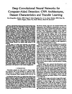
Fig. 5. Detections of the discovered part detectors on the dogs dataset. Green corresponds to the nose, red to the head and blue to the body of the dog. The last image is a failure case. Best viewed in color.
Table 1. Part localization error on the CUB-2011-200 dataset for our part strategy method w/ and w/o GMM for finding the activation centers, our method w/ and w/o restricting the localization to the bounding box (BB), and the method of [26] . In addition, we also show the performance of our approach for a CNN trained from scratch on CUB200-2011. Method Ours (GMM, BB) Ours (GMM, Full) Ours (MaxG, BB) Part Transfer [26] (BB) Ours (CNN from scratch)
Norm. Error 0.16 0.17 0.17 0.18 0.36
Fig. 6. Part localization examples from birds dataset. No bounding box and no geometric constraints for the part locations are used during the localization. The first three images are analyzed correctly, the belly and wing position are wrongly located in the fourth image. Best viewed in color.
dataset, the three discovered detectors seem to correspond to the nose (red), head (green), and body (blue). Especially the nose is identified reliably. For the birds dataset, we present four challenging examples in which only a small portion of the image contains the actual bird. In addition to this, the bird is often partially occluded. Nevertheless, our approach is able to precisely locate the head (red) and the legs (white). While there is more variance in the body (blue), wing (light blue), and tail (purple) location, they are still close to the real locations. The last example in Fig. 5 and Fig. 6 shows a failure case. Evaluating the Part Localization Error First, we are interested to what extent the learned part detectors relate to semantic parts. After identifying the spatially most related channel for each semantic part, we can apply our method to the test images to predict the location of semantic parts. The localization errors are given in Table 1. For calculating the localization error, we follow the
Part Detector Discovery in Deep Convolutional Neural Networks Training Testing Method Parts BBox Parts GT GT GT GT GT GT GT GT GT
GT GT GT GT GT GT GT
est. est. est. est. GT est.
Baseline (BBox CNN features) Berg et al. [9] Goering et al. [26] Chai et al. [29] Ours (part strategy) Ours (part strategy) Donahue et al. [5]
13
Recognition Rate 56.00% 56.78% 57.84% 59.40% 62.53% 62.67% 64.96%
est. Ours (part strategy) GT Ours (part strategy)
60.17% 60.55%
Baseline (global CNN features) est. Ours (counting) est. Ours (bounding box strategy)
41.60% 51.93% 53.75%
Table 2. Species categorization performance on the CUB200-2011 dataset. We distinguish between different experimental setups, depending on whether the ground-truth parts are used in training and whether the ground-truth bounding box is used during testing1 .
work of [26] and use the mean pixel error normalized by the length of the diagonal of the ground-truth bounding box. Our method achieves a significantly lower part localization error compared to [26] and a baseline using a CNN learned from scratch on the CUB200-2011 dataset only. A detailed analysis of the part localization error for each part is given in the supplementary materials including several observations about the channel-part correspondences: there are groups of parts that are associated with the same channel and there are parts, such as the beak and the throat, where we are twice as accurate as [26]. This indicates that the system can distinguish different bird body parts without direct training, which is a surprising fact given that we use a CNN trained for a completely different task. Evaluation for Part-based Fine-grained Classification We apply the presented part-based classification method to the CUB200-2011 dataset in order to evaluate to what extend the predicted part locations contribute to a higher accuracy. As can be seen in Table 2, our approach achieves a classification accuracy of 62.5%, which is one of the best results on CUB-2011-200 without fine-tuned CNNs. Whereas the method of [26] heavily relies on the ground-truth bounding box for part estimation, our method can also perform fine-grained 1
After submission, two additional publications [30,31] were published reporting 73.9% and 75.7% accuracy if part annotations are used only in training and no groundtruth bounding box is used during testing. Both of these works perform fine-tuning of the CNN models, which is not done in our case.
14
Marcel Simon, Erik Rodner, Joachim Denzler
classification on unconstrained full images without a manual preselection of the area containing the bird. These results are also shown in Table 2. As the main focus of this paper is the part localization, two more results are presented. First, the performance without using any part-based representation is a lower bound of our approach, since we also add global features to our feature representation. The recognition rate in this case is 56.0% for the constrained and 41.6% for the unconstrained setting. Second, the performance with groundtruth part locations is an upper bound, if we assume that human annotated semantic parts are also the best ones for automatic classification. In this case, the accuracy is 62.7% and 60.6%, respectively. The recognition rate of our approach with estimated part locations and the upper bound are nearly identical with a difference of only 0.2% and 0.5%, respectively. We also show the results in the case no ground-truth part annotations are provided for the training data. A baseline is provided by using CNN activations of the uncropped image for classification. The presented counting strategy as well as the bounding box strategy are able to significantly outperform this baseline by over 10% accuracy. The bounding box strategy performs best with only 6% less performance compared to the part strategy, which makes use of ground-truth part locations during training.
6
Conclusions
We have presented a novel approach for object part discovery and detection with pre-trained deep models. The motivation for our work was that deep convolutional neural network models learned on large-scale object databases such as ImageNet are already able to robustly detect basic shapes typically found in natural images. We exploit this ability to discover useful parts for a fine-grained recognition task by analyzing gradient maps of deep models and selecting activation centers related to annotated semantic parts or bounding boxes. After this simple learning step, part detection basically comes for free when applying the deep CNN to the image and detecting parts takes only a few seconds. Our experimental results show that in combination with a part-based classification approach this leads to an excellent performance of 62.5% on the CUB-2011200 dataset. In contrast to previous work [26], our approach is also suitable for situations when the ground-truth bounding box is not given during testing. In this scenario, we obtain an accuracy of 60.1%, which is only slightly less than the result for the restricted setting with given bounding boxes. Furthermore, we also show how to learn without given ground-truth part locations, making fine-grained recognition feasible without huge annotation costs. Future work will focus on dense features for the input image that can be obtained by stacking all gradient maps of a layer. This allows us to apply previous part-based models like DPM, which also include geometric constraints for the part locations. Furthermore, multiple channels can relate to the same part and our approach can be very easily modified to tackle these situations using an iterative approach.
Part Detector Discovery in Deep Convolutional Neural Networks
Acknowledgments donation.
15
This work was supported by Nvidia with a hardware
References 1. Krizhevsky, A., Sutskever, I., Hinton, G.: Imagenet classification with deep convolutional neural networks. In: Advances in Neural Information Processing Systems (NIPS). (2012) 1097–1105 2. Bengio, Y., Courville, A.C., Vincent, P.: Representation learning: A review and new perspectives. IEEE Transactions on Pattern Analysis and Machine Intelligence (PAMI) 35 (2013) 1798–1828 3. Bengio, Y.: Learning deep architectures for ai. Foundations and Trends in Machine Learning 2 (2009) 1–127 4. Zeiler, M.D., Fergus, R.: Visualizing and understanding convolutional networks. In: European Conference on Computer Vision (ECCV). (2014) 818–833 5. Donahue, J., Jia, Y., Vinyals, O., Hoffman, J., Zhang, N., Tzeng, E., Darrell, T.: Decaf: A deep convolutional activation feature for generic visual recognition. arXiv preprint arXiv:1310.1531 (2013) 6. Sermanet, P., Eigen, D., Zhang, X., Mathieu, M., Fergus, R., LeCun, Y.: Overfeat: Integrated recognition, localization and detection using convolutional networks. In: International Conference on Learning Representations (ICLR), CBLS (2014) Preprint, http://arxiv.org/abs/1312.6229. 7. Razavian, A.S., Azizpour, H., Sullivan, J., Carlsson, S.: CNN features off-the-shelf: an astounding baseline for recognition. arXiv preprint arXiv:1403.6382 (2014) 8. Felzenszwalb, P.F., Girshick, R.B., McAllester, D., Ramanan, D.: Object detection with discriminatively trained part-based models. IEEE Transactions on Pattern Analysis and Machine Intelligence (PAMI) 32 (2010) 1627–1645 9. Berg, T., Belhumeur, P.: Poof: Part-based one-vs.-one features for fine-grained categorization, face verification, and attribute estimation. In: IEEE Conference on Computer Vision and Pattern Recognition (CVPR). (2013) 955–962 10. Cortes, C., Vapnik, V.: Support-vector networks. Machine learning 20 (1995) 273–297 11. Erhan, D., Szegedy, C., Toshev, A., Anguelov, D.: Scalable object detection using deep neural networks. In: IEEE Conference on Computer Vision and Pattern Recognition (CVPR). (2014) Preprint, http://arxiv.org/abs/1312.2249. 12. Szegedy, C., Toshev, A., Erhan, D.: Deep neural networks for object detection. In: Advances in Neural Information Processing Systems (NIPS). Curran Associates, Inc. (2013) 2553–2561 13. Simonyan, K., Vedaldi, A., Zisserman, A.: Deep inside convolutional networks: Visualising image classification models and saliency maps. arXiv preprint arXiv:1312.6034 (2013) 14. Dalal, N., Triggs, B.: Histograms of oriented gradients for human detection. In: IEEE Conference on Computer Vision and Pattern Recognition (CVPR). (2005) 886–893 15. Wang, X., Yang, M., Zhu, S., Lin, Y.: Regionlets for generic object detection. In: IEEE International Conference on Computer Vision (ICCV). (2013) 17–24 16. Bourdev, L., Malik, J.: Poselets: Body part detectors trained using 3d human pose annotations. In: IEEE International Conference on Computer Vision (ICCV). (2009) 1365–1372
16
Marcel Simon, Erik Rodner, Joachim Denzler
17. Zhang, N., Farrell, R., Iandola, F., Darrell, T.: Deformable part descriptors for finegrained recognition and attribute prediction. In: IEEE International Conference on Computer Vision (ICCV). (2013) 729–736 18. Zhang, N., Paluri, M., Ranzato, M., Darrell, T., Bourdev, L.: Panda: Pose aligned networks for deep attribute modeling. In: IEEE Conference on Computer Vision and Pattern Recognition (CVPR). (2014) Preprint, http://arxiv.org/abs/1311. 5591. 19. Zou, W.Y., Wang, X., Sun, M., Lin, Y.: Generic Object Detection With Dense Neural Patterns and Regionlets. CoRR (2014) Preprint, http://arxiv.org/abs/ 1404.4316. 20. Jain, A., Tompson, J., Andriluka, M., Taylor, G.W., Bregler, C.: Learning human pose estimation features with convolutional networks. International Conference on Learning Representations (ICLR) (2014) Preprint, http://arxiv.org/abs/1312. 7302. 21. Toshev, A., Szegedy, C.: Deeppose: Human pose estimation via deep neural networks. In: IEEE Conference on Computer Vision and Pattern Recognition (CVPR). (2014) Preprint, http://arxiv.org/abs/1312.4659. 22. Sun, Y., Wang, X., Tang, X.: Deep convolutional network cascade for facial point detection. In: IEEE Conference on Computer Vision and Pattern Recognition (CVPR). (2013) 3476–3483 23. Lazebnik, S., Schmid, C., Ponce, J.: Beyond bags of features: Spatial pyramid matching for recognizing natural scene categories. In: IEEE Conference on Computer Vision and Pattern Recognition (CVPR). (2006) 2169–2178 24. Coates, A., Ng, A.: The importance of encoding versus training with sparse coding and vector quantization. In: Proceedings of the 28th International Conference on Machine Learning (ICML), ACM (2011) 921–928 25. Borji, A., Itti, L.: State-of-the-art in visual attention modeling. IEEE Transactions on Pattern Analysis and Machine Intelligence (PAMI) 35 (2013) 185–207 26. G¨ oring, C., Rodner, E., Freytag, A., Denzler, J.: Nonparametric part transfer for fine-grained recognition. In: IEEE Conference on Computer Vision and Pattern Recognition (CVPR). (2014) 27. Wah, C., Branson, S., Welinder, P., Perona, P., Belongie, S.: The Caltech-UCSD Birds-200-2011 Dataset. Technical Report CNS-TR-2011-001, California Institute of Technology (2011) 28. Liu, J., Kanazawa, A., Jacobs, D., Belhumeur, P.: Dog breed classification using part localization. In: European Conference on Computer Vision (ECCV). (2012) 172–185 29. Chai, Y., Lempitsky, V., Zisserman, A.: Symbiotic segmentation and part localization for fine-grained categorization. In: IEEE International Conference on Computer Vision (ICCV). (2013) 321–328 30. Zhang, N., Donahue, J., Girshick, R., Darrell, T.: Part-based r-cnns for fine-grained category detection. In: European Conference on Computer Vision (ECCV). (2014) 31. Branson, S., Horn, G.V., Belongie, S., Perona, P.: Bird species categorization using pose normalized deep convolutional nets. CoRR (2014) Preprint, http: //arxiv.org/abs/1406.2952.
Supplemental Materials: Part Detector Discovery in Deep Convolutional Neural Networks Marcel Simon, Erik Rodner, and Joachim Denzler Computer Vision Group, Friedrich Schiller University of Jena, Germany www.inf-cv.uni-jena.de
S1
Evaluating the Part Localization Error in Detail
The best matching channel as well as the localization errors are given in Table S1. For calculating the localization error, we follow the work of [26] and use the mean pixel error normalized by the length of the diagonal of the ground-truth bounding box. Interestingly, there are groups of parts that are associated with the same channel. The first group includes all parts near the head: beak, crown, forehead, left and right eye, breast, nape and throat. The second group is comprised of the left and right wing and the third one is the belly and the left and right leg. The back and the tail are each associated with a separate channel. This indicates that the system can distinguish different larger bird body parts, which is a surprising fact given that we use a CNN trained for a completely different task. In comparison to [26], we achieve a lower overall error with the benefit of our method most prominent in case of the beak and the throat. In case of the throat, the presented approach is more than twice as accurate as the one of [26]. The semantic part with the highest localization error is the tail, which seems to be challenging in general judging from the results of our competitor. A detailed part localization error analysis for a few selected parts is given in Fig. S1. In this plot, the sorted normalized errors for all test images are shown. The x-axis corresponds to the rank in the sorted error list, and the y-axis is the normalized distance to the ground-truth part location. The dotted lines are the results of [26] while the solid lines correspond to our approach. In case of the throat, the error of the presented approach is significantly lower and less than half in most cases. The other parts are located with a comparable accuracy.
18
Marcel Simon, Erik Rodner, Joachim Denzler Part
Channel
Normalized Euclidean error Ours Ours Ours Part transfer (GMM, BB) (GMM, Full) (MaxG, BB) [26] (BB)
Back
6
0.17
0.20
0.19
0.11
Beak
208
0.17
0.15
0.14
0.26
Belly
171
0.14
0.17
0.17
0.13
Breast
208
0.15
0.18
0.21
0.20
Crown
208
0.16
0.16
0.13
0.20
Forehead
208
0.16
0.14
0.12
0.24
Left eye
208
0.13
0.12
0.11
0.17
Left leg
171
0.15
0.16
0.15
0.13
Left wing
73
0.18
0.20
0.22
0.15
Nape
208
0.15
0.16
0.17
0.13
Right eye
208
0.13
0.12
0.11
0.31
Right leg
171
0.16
0.16
0.15
0.15
Right wing
73
0.17
0.20
0.21
0.13
Tail
54
0.33
0.36
0.35
0.28
Throat
208
0.10
0.11
0.13
0.23
Average
-
0.16
0.17
0.17
0.18
Table S1. Part localization error on the CUB-2011-200 dataset for our method w/ and w/o GMM for finding the activation centers, our method w/ and w/o restricting the localization to the bounding box (BB), and the method of [26]. Tail (our approach) Belly (our approach) Throat (our approach) Tail (Goering) Belly (Goering) Throat (Goering)
1.5 of part detection
Normalized euclidean error
2
1
0.5
0
0
0.2
0.4
0.6
0.8
1
Normalized rank
Fig. S1. Distribution of the part localization error: the sorted normalized localization errors for the tail, the belly, and the throat compared to the approach of [26] is shown.