FAST MORPHOLOGICAL ATTRIBUTE OPERATIONS USING TARJAN’S UNION-FIND ALGORITHM
MICHAEL H. F. WILKINSON and JOS B. T. M. ROERDINK Institute for Mathematics and Computing Science, University of Groningen, P.O. Box 800, 9700 AV, Groningen, The Netherlands
Abstract. Morphological attribute openings and closings and related operators are generalizations of the area opening and closing, and allow filtering of images based on a wide variety of shape or size based criteria. A fast union-find algorithm for the computation of these operators is presented in this paper. The new algorithm has a worst case time complexity of O(N log N ) where N is the image size, as opposed to O(N 2 log N ) for the existing algorithm. Memory requirements are O(N ) for both algorithms. Key words: area operators, attribute operators, granulometries, union-find algorithm.
1. Introduction Morphological attribute openings, thinnings and granulometries were introduced by Breen and Jones [1] as a generalization of morphological area operators proposed by Vincent [8, 9]. Attribute openings are most easily understood in the binary case. Unlike structural openings, attribute openings are shape preserving, because they simply test whether a connected component satisfies some increasing criterion T . If it does, it is retained, if not, it is removed. In the case of the area opening, the area of each component is compared to some threshold value λ, and if the area of the component is larger, it is retained. The flexibility of this methodology is shown in Figure 1. In this figure a binary image of bacteria is filtered using three attribute openings, each of which would remove all squares smaller than 11 × 11 pixels. The first is the area opening, with λ = 121. All small bacteria have been removed in the resulting image. By contrast, the attribute opening using the criterion that the moment of inertia I must be larger than λ = 114 /6, removes most of the smaller components, but not the elongated ones. Attribute opening using √ the length of the diagonal of the minimum enclosing rectangle as criterion, with λ = 242, has similar results. The algorithm Breen and Jones derive for their wider class of operators is based on Vincent’s pixel queue algorithm for area operators. Recently, a new algorithm for area openings and closings has been developed [5], which is based on Tarjan’s unionfind algorithm [7]. It was found that the union-find based algorithm was between 2 and 10 times faster than the original algorithm on the images tested. Furthermore, the computational burden of the new algorithm was practically independent of the size criterion λ used, or the image content. By contrast, Vincent’s algorithm is particularly sensitive to the presence of linear structures in the image, in which case the computing time rises almost linearly with λ.
312
MICHAEL H. F. WILKINSON AND JOS B. T. M. ROERDINK
(a)
(b)
(c)
(d)
Fig. 1. Attribute openings of an image of bacteria: (a) a binary image of 256 × 256 pixels; attribute using (b) area A ≥ 121; (c) Moment of inertia I ≥ 114 /6, corresponding √ to that of an 11 × 11 square, and (d) length of diagonal of minimum enclosing rectangle D ≥ 242. Structural opening of (a) by an 11 × 11 square structuring element removes all objects.
In this paper we extend the union-find algorithm to the wider class of attribute openings and closings. Later work will focus on extension to thinnings and thickenings, and granulometries or size distributions. 2. Attribute Morphology: Theory The theory of attribute operators is given only briefly here. For a more thorough discussion the reader is referred to [1]. Here we will first discuss binary attribute openings and closings, and then the extension to the grey scale case. Binary attribute openings are based on binary connected openings. Let the set X ⊆ M denote a binary image with domain M. The binary connected opening Γx (X) of X at point x ∈ M yields the connected component of X containing x if x ∈ X, and ∅ otherwise. Thus Γx extracts the connected component to which x belongs, discarding all others. Breen and Jones then use the concept of trivial openings ΓT , which use an increasing criterion T to accept or reject connected sets. A criterion T is increasing if the fact that C satisfies T implies that D satisfies T for all D ⊇ C. The trivial opening ΓT of a connected set C with increasing criterion T is just the set C if C satisfies T , and is empty otherwise. Furthermore, ΓT (∅) = ∅. The binary attribute opening is defined as follows. Definition 1 The binary attribute opening ΓT of set X with increasing criterion T is given by [ ΓT (X) = ΓT (Γx (X)) (1) x∈X
It can be shown that this is an opening because it is increasing, idempotent, and anti-extensive [1]. The attribute opening is equivalent to performing a trivial opening on all connected components in the image. A generalization to grey scale can be made by first defining thresholded images Xh (f ), Xh (f ) = {x ∈ M|f (x) ≥ h} (2)
313
FAST ATTRIBUTE OPERATORS
1
1
Xh
1
M h= P h= L h M2h = P2h = L2h
h
Xh' h' h"
P1h' L
1 h"
Xh"
(a)
(b)
Fig. 2. One dimensional discrete image with grey levels h > h0 > h00 to illustrate the definitions of level components, regional maxima, peak components, and the threshold images: (a) double arrows indicate three level components L1h , L2h and L1h00 ; the former two are also both peak components Ph1 and Ph2 and regional maxima at level h; a further peak component Ph10 at level h0 is also shown; (b) shows the threshold sets Xh , Xh0 , and Xh00 in relationship to the grey scale image.
where the grey scale image f is a mapping from the image domain M to Z∪{−∞, ∞}. Definition 2 The grey scale attribute opening γ T of image f with increasing criterion T is given by (γ T (f ))(x) = max{h|x ∈ ΓT (Xh (f ))}. (3) Grey scale attribute closings can easily be defined by a duality relationship with the grey scale attribute openings [5]. 3. Algorithms Before going into the details of the algorithms, we first define a level component Lh at level h of a grey scale image f as a connected component of the set of pixels {p ∈ M|f (p) = h}. A regional maximum Mh at level h is a level component no members of which have neighbors larger than h. A peak component Ph at level h is a connected component of Xh (f ). At each level h there may be several such components, which will be indexed as Lih , Phj and Mhk , respectively, with i, j, and k from some index set. It can be seen that any regional maximum Mhk is also a peak component, but the reverse is not true. Examples of these three types of components, and of the threshold sets Xh (f ) are given in Figure 2. All level components Lih at level h are of course subsets of some peak component j Ph ⊂ Xh (f ) at the same level h. However, for a given criterion T , not necessarily all Lih ⊂ ΓT (Phj ), because not all Phj need meet the criterion T . It can be seen from (3), that not all level components are necessarily affected by a grey scale attribute opening. Only those Lih which are not subsets of a peak component Phj which
314
MICHAEL H. F. WILKINSON AND JOS B. T. M. ROERDINK
(a)
(b)
(c)
(d)
(e)
(f)
(g)
Fig. 3. Processing nested maxima by the pixel queue algorithm, assuming only the peak at full width meets the criterion: (a) original image; (b-f) situation after processing the first, second, third, fourth, and fifth maximum from the left. At each stage the pixels indicated by the double arrows have been inspected. After visiting the current maximum, the algorithm first inspects the pixels to the left of the maximum, because the valley to the right is lower. This results in a frequent rescanning of pixels of the left-most regional maxima. (g) 16 × 16 pixel image showing nested maximum structure on which the computational burden is expected to be O(N 2 log N ).
meets the criterion T must be changed in grey level by γ T . In other words, all Lih ⊂ ΓT (Phj ) ⊂ ΓT (Xh (f )) must be left unaltered. If we assume that the peak component Ph10 in Figure 3 meets the criterion, the level component labeled L1h00 in the same figure will remain unaltered. This is because h00 < h0 , so that Ph10 ⊂ Ph100 (the latter is not shown in the figure), and since T must be increasing in the case of a grey scale attribute opening, Ph100 must meet T . By contrast, assume that Ph1 = Mh1 = L1h does not meet the criterion, and therefore L1h 6⊂ ΓT (Ph1 ) since ΓT (Ph1 ) = ∅. Then the grey level of L1h must be altered to h0 , because Ph10 ⊃ L1h is the smallest peak component containing L1h which meets T . 3.1. The Pixel Queue Algorithm The pixel queue based algorithms for morphological area and attribute operators are given in some detail elsewhere [1, 5, 8, 9], so we will describe them only briefly. The source code of our implementations is available on request. Briefly, the image is first scanned using a pixel queue to create a list of all regional maxima Mhk . After this, all Mhk are processed sequentially. This is done by growing a peak component Phj1 , h1 ≤ h around a seed pixel within the maximum Mhk using a priority queue. As each pixel is added to the growing region, its neighbors which do not (yet) belong to the region are put in the priority queue, from which they are retrieved in reverse grey level order. The process of adding pixels pauses whenever the next pixel taken from the priority queue has a grey level h00 different from the current level h0 . If h00 > h0 , the region grown so far is not a peak component Phj0 at level h0 . All the grey levels of pixels found so far are set to h0 , and the maximum Mhk from which the region was grown is removed from the list. If h00 < h0 , the region grown so far is a peak component at h0 , which is subsequently checked against the criterion. If the criterion is met, the grey level of all pixels p ∈ Phj0 are set to h0 , and Mhk is removed from the list. Otherwise, the routine continues adding new pixels at level h00 . The algorithm terminates when all maxima have been processed. One problem which occurs is that pixels may be visited more than once if nested
FAST ATTRIBUTE OPERATORS
315
maxima exist, especially if the attribute threshold λ is large. This effect can be seen in Figure 3. In this one-dimensional example, the algorithm processes the maxima from left to right, and each time only detects that the growing region is not a peak component after having re-visited all pixels visited by the previous region-growing loop. If λ is chosen so that the entire image (of N pixels) is the smallest set satisfying the criterion, it is possible to construct an image in which each pixel is processed O(N ) times. A two-dimensional example can be seen in Figure 3g. At each visit a pixel has to be inserted into and retrieved from a priority queue of length of order √ N . In that case we arrive at a worst case running time of O(N 2 log N ). Strictly speaking, this effect is due to awkward arrangement of the depths of the valleys between the maxima, not to the heights of the maxima. Had all the maxima in figure 3(a) been given the same height (as is the case in figure 3(g)), the problem still remains. Processing the maxima in order of grey level does not solve the problem. The algorithm requires a label image of N pixels, and a (priority) queue also of N pixels in the worst case. Therefore its memory requirements are O(N ). 3.2. The Union-Find Method Tarjan [7] presents the union-find algorithm which provides a general method for keeping track of disjoint sets. It allows performing set-union operations on sets which are in some way equivalent, while ensuring that the end product of such a union is disjoint from any other set. Since connected components and level components in an image are by definition disjoint sets, the union-find algorithm lends itself to any image processing method which is defined by such image components. Dillencourt et al. [2] have shown that the union-find algorithm can be used for efficient connected component labeling of arbitrary image representations. Fiorio and Gustedt propose a similar algorithm [3], and Meijster and Roerdink [4] adapted the algorithm to levelcomponent labeling. Since attribute openings and closings are connected filters, their operation can be defined directly in terms of connected components in the binary case and level components in the grey scale case. This means Tarjan’s algorithm can be adapted to attribute openings. This is born out by the application of the algorithm to area openings [5]. Tarjan uses tree structures to represent sets. Each non-root node in a tree points to its parent, while the root is flagged in some way. Two objects x and y are members of the same set if and only if x and y are nodes of the same tree, which is equivalent to saying that they share the same root. There are four important operations. − Makeset(x): Create a new singleton set {x}. − FindRoot(x): Return the root element of the set containing x. − Union(x,y): Compute the union of the two sets containing x and y. − Equiv(x,y): determine whether x and y satisfy some equivalence criterion. For level component labeling the algorithm becomes: for pixels p do { MakeSet(p); for all neighbors n
= lambda ) ) { parent[q]=INACTIVE; DisposeAuxData(auxdata[q]); } MakeSet(p); for all neighbors n