Abinit [2]: This software was developed using a popular formulation of DFT
known as KS-. DFT (Kohn-Sham). It is currently run by. Xavier Gonze and written
in ...
DFT Software: Who, What, and How Much Brad Hubartt Introduction:
Doing pretty much anything in quantum mechanics is going to involve the wave equation of the system. Using the wave equation in a large system is going to be very difficult or impossible, if the wave equation is even known. This essentially rules out using quantum mechanics in biophysics/chemistry. A new quantum model is needed for these systems. Density Functional Theory (DFT) [4][6][9][12] is such a model. It involves using the probability density functions of the electrons in a molecule to determine other properties of the molecule. Instead of solving problems with wave equations for each electron it uses the probabilities of electrons being at different locations. If the wave function is not known many implementations of DFT will allow for Gaussians to be used in their place.
DFT works by minimizing functions of functions, functionals, to determine the ground state of a molecule. Instead of using functionals based upon each individual electron, a pseudopotential is used to simplify the calculation. Additionally it can calculate forces and has been expanded to include timedependence [13]. Time-dependent DFT makes simulations of molecular dynamics possible. Molecular dynamics are of particular interest as nothing in a biological system is static; proteins are floating around in a solution and constantly interacting with different ions. Methods:
This is a seemingly wonderful theory, but how is it implemented? It is not particularly useful if every equation has to be solved by hand at each iteration. First, where does the electron density come from? Kohn and Sham came up with an approach for this which is how Kohn-Sham DFT (KS-DFT)
was constructed [11]. KS-DFT takes the original energy ! functional:
E[ρ] = T [ρ] +
Vext (r)ρ(r)dr + VH [ρ] + Exc [ρ]
where T is the kinetic energy, Vext is the external potential, VH is the Hartree energy, Exc is the exchange correlation energy, and ρ is the charge density. ρ is what Kohn and Sham modified. They derived the following three equations: ρ(r) =
N ! ! i
s
|ψi (r, s)|2
!2 2 − ∇ ψi (r, s) + vef f (r)ψi (r, s) = #i ψi (r, s) 2m " δExc [ρ] ρ(r! ) 2 vef f (r) = Vext (r) + e dr! + ! |r − r | δρ
The first one is exactly what anyone would expect, the second is Schrödinger’s equation, and the third is the actual potential at a given location based upon the externally applied potential, the charge density, and the correlation energy. ρ can be solved for by integrating over these three equations with an RK4 [10] or something equivalent. Often the wave equation is replaced with a Gaussian to simplify things.
Another technique used to simplify DFT is replacing all-electron systems with a pseudopotential. A pseudopotential is an approximation of the Coulombic potential from the non-valence electrons. In chemistry the valence electrons are the ones that actually form bonds and cause reactions; the non-valence electrons are just there for the potential field (obviously a gross oversimplification). Pseudopotentials are used when generating a self-consistent field. Pulay Mixing [3] (also called Direct Inversion of Iterative Subspace) is a non-linear mixing technique used for large SCF problems.
Hubartt 1
Instead of having to store a giant hessian for the system this algorithm works with an amount n (user specified integer) of charge density vectors. Through a few linear operations a final charge density vector is computed. The computational benefits of Pulay Mixing are increasingly noticeable the large the system becomes as the hessian grows as nelectrons squared versus needing only a handful of vectors for Pulay mixing. The actual algorithm for Pulay mixing is in reference [3] and [4].
No one wants to solve this by hand, the natural place for this theory is in computer simulations. A quick internet search reveals a few dozen pieces of software for solving these systems. Each one comes with its own quirks, learning curves, availability of documentation, open/closed-source, and whether the originator of the software has been banned for life from using it (amongst other people). The purpose of this paper is to select a few of these programs to discuss how they work. Featured programs were picked fairly randomly from a list of available ones with little bias save one. Abinit [2]:
This software was developed using a popular formulation of DFT known as KSDFT (Kohn-Sham). It is currently run by Xavier Gonze and written in FORTRAN. Dozens of variables are available for customizing the input conditions of a system. A few of the basic variables are: acell, angdeg, ecut, natom, nband, and iscf; essentially every property that can change from one system to the next is customizable if desired. Keep in mind that most of these have fairly generic default settings. acell gives the size of the unit cell usually in Borh radii (other units are allowed if you specify them), angdeg sets the angles between the three primitive vectors for the unit cell, ecut sets a maximum value for the kinetic energy of the system, natom is the number of atoms in a
unit cell, nband is the number of bands to be considered, and iscf determines which mixing algorithm is used to find a self-consistent field. The iscf variable by default is set to use Pulay Mixing. Other mixing algorithms are built into Abinit that are simpler than Pulay which could give mixed results based upon the size and complexity of the system. Other more advanced input variables are built into Abinit including the Bravais lattice type, how to calculate the Berry phase, units for energy, various dielectric properties, etc... ABINIT has two different pseudopotentials built into it for each element. Additionally, it has multiple algorithms to calculate a new pseudopotential if one is desired.
What does it output? Besides a confirmation of all the input parameters it has a hefty amount of items to output. The first is the point symmetry group and the Bravais lattice type. The Bravais lattice, along with many of the input parameters, are geared more for solid state physics than molecular physics/chemistry. It has to do with the crystal structure of the material being analyzed. The point symmetry group has to do with how many rotational symmetries exist, again this is geared more for crystal structures. After this comes the real output. It gives the atomic positions in cartesian coordinates, energy gradients, forces in eV/ Angstrom, eigenvalues of each band for each k point, minimum and maximum charge densities, a list of all the different energy components, and the stress (average force per area) tensor in GPa.
Gaussian:
This company’s program has had quite the history. It was originally developed by noble laureate John Pople in 1971 at Carnegie Mellon in FORTRAN. In the beginning the source was open and freely distributed to any university that wanted to use it. This is far from the present case. The program is now somewhat closed-source and sold by Hubartt 2
Gaussian Inc. under a fairly restrictive license. Various stipulations of the license are: not being allowed to disclose how fast the program is, work on any “competing” program, or allow anyone that is banned from using Gaussian to use your copy. Who exactly would be banned from using this? Pople (the creator!) is banned from using it, as are Princeton and CalTech along with many other universities and individuals. The official list of bannings is kept at www.bannedbygaussian.org. As it is illegal to discuss how fast this program is, any judgement as to whether Gaussian is a good program that is worth the $4500-36,000 (academic and industry prices for OS X version) for a site license is difficult to determine. It is especially hard to justify this price when there are open-source programs that are freely available. This company has established a huge barrier of entry for anyone wishing to get into the field. With the risk of being banned from using this software a clear danger, it is hard to imagine anyone using this software. Despite this, many groups do use Gaussian for their DFT calculations[7]. Quantum Espresso (QE) [15]:
QE is another open-source, free software suite for DFT. It is operated through a collaboration between MIT, Princeton (probably why they are banned from Gaussian), and multiple European Universities; it is coordinated by Paolo Giannozzi. It is written in a combination of C++ and FORTRAN. C++ is used to make the program object-oriented, very modular, and easier to learn initially with bit of FORTRAN for speed boosts. Just as with Abinit, QE uses KS-DFT and provides 75 pseudopotentials. Additionally, they provide software to generate a new or other pseudopotential as needed.
QE goes a step further with its calculations and allows for molecular dynamics to occur. These are based upon the
forces calculated at a given time-step with DFT and then integrated via a Verlet algorithm. The timescale for these dynamics is small, on order of picoseconds, but it is a start.
For visualizations the output files can be imported to a variety of additional programs. These allow for 3D overlays of the electron densities with molecular structures. One such program, gOpenMol [8] produced Fig 1.
Fig. 1 Electron density of the aspirin molecule
Setting up the input for QE is not particularly difficult. The user specifies the element(s) being used, which pseudopotential to use, the Bravais lattice, the k-point locations of the atoms in the 1st Brillouin zone (locations of the atoms in the inverse lattice), and other characteristics of their system. Many common lattices can be found on their website or on a few other databases that they refer the user to. Current Biophysics Uses:
The purpose of this paper was to describe a few of the many choices in software that are currently available for solving DFT calculations for biological molecules. How exactly would someone go about doing that and what would they gain? Using the crystal structure of a protein (obtainable freely online through the Protein Data Bank) the location of each amino acid would be known, therefore the location of Hubartt 3
each atom is known. Putting all of this information into anyone of the aforementioned programs would allow for a computation of the electron density in that protein [7]. It would be a long computation since most proteins would consist of hundreds of atoms, but on a large cluster of computers it is possible ([7] used Gaussian for their calculations which means no computation times were given). Just as with any other system, the internal Coulombic forces of the protein would be calculated, allowing the stability of that conformation to be determined. My own idea:
Beyond the realm of known structures though, there might be use for DFT with finding native states of proteins. There are many protein folding models out there with varying levels of simplification. The model I currently am working with is the HP model (hydrophobic hydrophilic respectively). In this model all of the amino acids are declared to be either H or P and then a folding simulation is run until a final conformation is reached. Due to the over simplification of this model (ignoring external potentials, crowding effects, ...) it is possible to find multiple conformations of equal energy. What could then be done is to translate these final conformations of Hs and Ps back to their original amino acid sequence, input this into Quantum Espresso, and determine the internal forces on each of them. The conformation with the lowest forces, if one is found, probabilistically would more likely be the native state of the protein.
Hubartt 4
References: 1. John S. Tse AB INITIO MOLECULAR DYNAMICS WITH DENSITY FUNCTIONAL THEORY. (2003).at 2. abinit. at 3. Pulay, P. Convergence acceleration of iterative sequences. the case of scf iteration. Chemical Physics Letters 73, 393-398(1980). 4. Yang, R.G.P.A.W. Density-Functional Theory of Atoms and Molecules. (Oxford University Press: New York, 1989). 5. Mattsson, A.E. et al. Designing meaningful density functional theory calculations in materials science—a primer. Modelling and Simulation in Materials Science and Engineering 13, R1-R31(2005). 6. March, N.H. Electron Density Theory of Atoms and Molecules. (Academic Press: 1992). 7. Dudev, T. et al. First-second shell interactions in metal binding sites in proteins: a PDB survey and DFT/CDM calculations. J Am Chem Soc 125, 3168-80(2003). 8. g0penMol — CSC. at 9. Teller, E. On the Stability of molecules in the Thomas-Fermi theory. Rev. Mod. Phys. 34, 627–631(1962). 10. Runge-Kutta Method -- from Wolfram MathWorld. at 11. Kohn, W. & Sham, L.J. Self-Consistent Equations Including Exchange and Correlation Effects. Phys. Rev. 140, A1133(1965). 12. Lieb, E.H. & Simon, B. The Thomas-Fermi theory of atoms, molecules and solids. Adv. in Math. 23, 22–116(1977). 13. Tavernelli, I. et al. Time-Dependent Density Functional Theory Molecular Dynamics Simulations of Liquid Water Radiolysis. ChemPhysChem 9, 2099-2103(2008). 14. The Mathematics of DIIS. at 15. P. Giannozzi et al., http://www.quantum-espresso.org
Hubartt 5