Analytical Biochemistry 287, 243–251 (2000) doi:10.1006/abio.2000.4879, available online at http://www.idealibrary.com on
Estimation of Protein Secondary Structure from Circular Dichroism Spectra: Inclusion of Denatured Proteins with Native Proteins in the Analysis Narasimha Sreerama,* Sergei Yu. Venyaminov,† and Robert W. Woody* ,1 *Department of Biochemistry and Molecular Biology, Colorado State University, Fort Collins, Colorado 80523; and †Department of Pharmacology, Mayo Foundation, Rochester, Minnesota 55905
Received April 7, 2000
We have expanded our reference set of proteins used in the estimation of protein secondary structure by CD spectroscopy from 29 to 37 proteins by including 3 additional globular proteins with known X-ray structure and 5 denatured proteins. We have also modified the self-consistent method for analyzing protein CD spectra, SELCON3, by including a new selection criterion developed by W. C. Johnson, Jr. (Proteins Struct. Funct. Genet. 35, 307–312, 1999). The secondary structure corresponding to the denatured proteins was approximated to be 90% unordered, owing to the spectral similarity of the denatured proteins and unordered structures. We examined the thermal denaturation of ribonuclease T1 by CD using both the original and expanded sets of reference proteins and obtained more consistent results with the expanded set. The expanded set of reference proteins will be helpful for the determination of protein secondary structure from protein CD spectra with higher reliability, especially of proteins with significant unordered structure content and/or in the course of denaturation. © 2000 Academic Press
Key Words: protein secondary structure; SELCON; CD analysis; protein CD; unordered structure.
One of the most successful applications of CD, the structural characterization of proteins, depends upon the remarkable sensitivity of the far-UV CD to the backbone conformation of proteins; the far-UV CD of a protein generally reflects the secondary structure content of the protein. Various empirical methods have been developed for analyzing protein CD spectra for 1 To whom correspondence should be addressed. Fax: (970) 4910494. E-mail:
[email protected].
0003-2697/00 $35.00 Copyright © 2000 by Academic Press All rights of reproduction in any form reserved.
quantitative estimation of the secondary structure content (1–20), and various aspects of secondary structure analysis have been reviewed (21–25). Methods have also been developed to estimate the number of secondary structural segments in proteins (19), and to assign the protein tertiary structure class from the analysis of far-UV CD spectra (26, 27). The basic principle involved in the analysis of protein CD spectra, and used in the estimation of secondary structure fractions, is that the protein CD spectrum (C ) can be expressed as a linear combination of CD spectra of individual secondary structure components (k), B k , C ⫽ ¥ f k B k , where f k is the fraction of the secondary structure k. Spectra of model polypeptides or of a set of reference proteins with known structures are used to determine the component secondary structure spectra, B k . The most successful methods use the CD spectra of a set of reference proteins with known structures, and the secondary structure fractions for the reference proteins are determined from the corresponding crystal structure. The following assumptions are involved in these methods: (1) the contributions from individual secondary structures are additive; (2) the ensemble-averaged solution structure and the time-averaged solid-state X-ray structure are equivalent; (3) the effect of the tertiary structure on CD is negligible; (4) the CD contributions from nonpeptide chromophores do not influence the analysis; (5) effects of the geometric variability of the secondary structures need not be explicitly considered. Although assumptions 1–3 are generally valid, assumptions 4 and 5 are likely to be incorrect in many cases (28, 29). This is the reason that flexible basis methods (variable weighting of the reference proteins (7), variable selection (9, 11, 15, 17–20) in which a large number of subsets of the reference set are used with the results subjected to tests to identify good solutions, and neural networks 243
244
SREERAMA, VENYAMINOV, AND WOODY
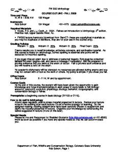
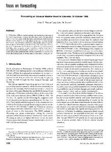
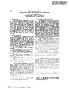
FIG. 1. CD spectra of five denatured proteins included in the Exp37 reference protein set. The proteins are: apocytochrome c, 5°C (short dashes); apocytochrome c, 90°C (long dashes); staphylococcal nuclease, 6°C (solid); staphylococcal nuclease, 70°C (dot– dash); and oxidized ribonuclease, 20°C (dotted).
(14, 16, 18)) have largely displaced fixed basis methods (1– 6, 8, 10, 12, 13). Although the flexible basis methods do not explicitly determine the CD spectra of individual secondary structural components (B k ), they implicitly assume such spectra, containing the effects of distortions, side chains, and end effects, adapted to the protein being analyzed. By contrast, a fixed reference set cannot take these variations into account. A reference protein set with a good representation of CD spectral features and secondary structural combinations is desirable for a good analysis. Different sets of reference proteins, with the number of proteins varying from 15 to 33 and having a good representation of ␣-rich, -rich, and mixed-␣ proteins, have been used in secondary structure analyses. In one case, four denatured protein CD spectra were included in a set of 16 reference proteins (30). We have extended the set of 29 reference proteins, used in our SELCON3 method, by adding 3 native proteins and 5 denatured proteins. We have also modified the SELCON3 method, introducing a new criterion for selecting valid solutions based on helical content developed by Johnson (20). The method and the reference protein set described in this paper were used to analyze changes of secondary structure in the course of thermal unfolding of ribonuclease T1.
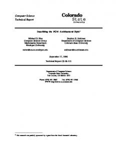
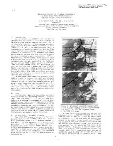
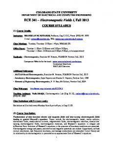
lysozyme (2lzm), triosephosphate isomerase (3tim), lactate dehydrogenase (6ldh), lysozyme (1lys), thermolysin (8tln), cytochrome c (5cyt), phosphoglycerate kinase (3pgk), EcoRI endonuclease (1eri), flavodoxin (1fx1), subtilisin BPN⬘ (1sbt), glyceraldehyde 3-phosphate dehydrogenase (3gpd), papain (9pap), subtilisin novo (2sbt), ribonuclease A (3rn3), pepsinogen (2psg), -lactoglobulin (1beb), ␣-chymotrypsin (5cha), azurin (1azu), elastase (3est), ␥-crystallin (4gcr), prealbumin (2pab), concanavalin A (2ctv), Bence–Jones protein (1rei), tumor necrosis factor (1tnf), superoxide dismutase (2sod), and ␣-bungarotoxin (2abx). The original set is referred to as Org29. Three globular proteins, colicin A (1col), green fluorescent protein (1ema), and rat intestinal fatty acid-binding protein (1ifc), were added to the Org29 reference proteins, bringing the total number of globular proteins to 32; this set is referred to as Exp32. CD spectra. CD spectra of the original 29 proteins were kindly provided by Dr. W. C. Johnson, Jr. The CD spectra of the three globular proteins added to the set of reference proteins were taken from Sreerama et al. (19). CD spectra of five denatured proteins were added to Exp32, bringing the number of CD spectra to 37, and this set is referred to as Exp37. The CD spectra of acid-denatured bovine apocytochrome c at 5 and 90°C, acid-denatured staphylococcal nuclease at 6 and 70°C, and acid-denatured oxidized ribonuclease at 20°C were taken from Privalov et al. (31). These five CD spectra are shown in Fig. 1. The CD spectra of ribonuclease T1 (RNase T1) at pH 5.0 and at different temperatures were measured at the Mayo Foundation on a J-710 spectropolarimeter in quartz cells of 0.01- to 0.02-cm pathlengths, using the following parameters: 2-s response; 20 nm/min scan speed; 0.1-nm data acquisition interval; 5 accumulations; 2-nm bandwidth. The CD spectra were smoothed using the noise reduction routines provided with the J-710 spectropolarimeter. CD spectra of RNaseT1 at different temperatures are given in Fig. 2.
MATERIALS AND METHODS
Reference proteins. Our original reference set consisted of 29 proteins. The proteins and the X-ray structures used (PDB 2 code in parenthesis) are: myoglobin (4mbn), hemoglobin (2mhb), hemerythrin (2hmz), T4 Abbreviations used: PDB, Protein Data Bank; ␦, root mean square deviation; r, correlation coefficient; Org29, original 29 reference proteins; Exp32, set of 32 globular reference proteins; Exp37, set of 37 reference proteins; SVD, singular value decomposition; ␣ R, regular ␣ helix; ␣ D, distorted ␣ helix;  R, regular  strand;  D, distorted  strand; T, turns; U, unordered; DSSP, a computer program for defining secondary structure of proteins. 2
FIG. 2. CD spectra of ribonuclease T1 during the course of thermal denaturation in 20 mM NaAc buffer at pH 5.0. The temperatures (°C) are shown along with the spectra.
PROTEIN CIRCULAR DICHROISM ANALYSIS
Secondary structure. The secondary structure assignments from DSSP (32) were used to determine the secondary structure fractions of the globular proteins in the reference set as described by Sreerama et al. (19). The ␣-helical and -sheet structures were split into regular and distorted classes by considering four residues per ␣ helix and two residues per  strand distorted. Our grouping of DSSP assignments gave us six secondary structural classes: regular ␣ helix, ␣ R; distorted ␣ helix, ␣ D; regular  strand,  R; distorted  strand,  D; turns, T; and unordered, U. The secondary structure of the denatured proteins was approximated to be 90% unordered and 2% of each of the remaining secondary structures, since structures for the denatured proteins are unavailable. CD analysis. The protein to be analyzed for secondary structure fractions was removed from the reference protein set and the secondary structure fractions were determined from its CD spectrum using the other members of the reference set, following the self-consistent method, SELCON3. In the self-consistent method (15) the spectrum of the protein analyzed is included in the matrix of CD spectral data, and an initial guess, the structure of the reference protein having the CD spectrum most similar to that of the protein analyzed, is made for the unknown secondary structure. The matrix equation relating the CD spectra to the secondary structure is solved by the singular value decomposition (SVD) algorithm (33), with variable selection (9) in the locally linearized model (11). Solutions are obtained by varying the reference proteins and/or the number of SVD components retained. The performance of the analysis was characterized by RMS deviations (␦) and correlation coefficients (r) between the X-ray (DSSP, 32) and CD estimates of secondary structure fractions for different secondary structure types. These are denoted by ␦ k and r k , where k is one of the secondary structural types considered. Overall performance of the analysis for a given set of secondary structure fractions was determined by considering all secondary structure fractions collectively, and these are given by ␦ and r. The RMS deviations and correlation coefficients were calculated using the equations
␦⫽
冑
¥ i 共f iCD ⫺ f iX兲 2 N
and
r⫽
N ¥ i 共f iCD ⫻ f iX兲 ⫺ ¥ ij 共f iCD ⫻ f jX兲
冑
关N ¥ i 共f iCD兲 2 ⫺ 共¥ i f iCD兲 2 兴 ⫻ 关N ¥ i 共f iX兲 2 ⫺ 共¥ i f iX兲 2 兴
,
245
where f iCD and f iX are CD and X-ray estimates for secondary structure types of N reference proteins. RESULTS AND DISCUSSION
SELCON3 Program The variable selection procedure as implemented in the self-consistent method yields a set of solutions as the number of reference proteins and the number of SVD components are varied. Four selection criteria are used to find valid solutions among the solutions given by the self-consistent method. They are: Sum rule, 兩¥ f k ⫺ 1.0兩 ⱕ 0.05, where f k is the fraction of secondary structure k; Fraction rule, f k ⱖ ⫺0.025; Spectral rule, ␦ CD (RMS difference between the experimental spectrum and the calculated spectrum) ⱕ0.25⌬⑀; and Helix rule (20), fraction of helix ( f ␣ ) is in a range determined from the helix fraction obtained with all reference proteins in the analysis ( f ␣HJ). The first two criteria have been derived by relaxing the physically meaningful constraints requiring that each fraction should be positive and the sum of all fractions should be unity. These selection criteria are incorporated in a stepwise manner in SELCON3 as follows: (a) Considering all proteins and five SVD components, the helix fraction ( f ␣HJ) is determined by the SELCON method. The output corresponds to that of the original method of Hennessey and Johnson (8). (b) The self-consistent method, with the incorporation of variable selection in the locally linearized formalism (11), is used to estimate all secondary structure fractions. Valid solutions satisfy the Sum rule and the Fraction rule. If at least one solution is not obtained, the rules are relaxed. The process is iterated for self-consistency. The results correspond approximately to those from the original SELCON (15) and SELCON1 (18) programs. (c) Solutions obtained from the SELCON method, at the end of step b, are screened using the Spectral rule. If at least one solution is not obtained, this rule is relaxed. The results are similar to those from SELCON2 program (Sreerama and Woody, unpublished results). (d) The Helix rule (20) is now applied to further screen solutions from step c. From H min, H max, and H ave, determined from solutions at the end of step c, and the helix content from step a, f ␣HJ, helix limits for valid solutions are determined. If f ␣HJ ⬎ 0.65, then valid solutions have f ␣ ⬎ 0.65. If 0.65 ⬎ f ␣HJ ⬎ 0.25, then valid solutions have f ␣ ⫽ ( f ␣HJ ⫹ H max)/2 ⫾ 0.03. If 0.25 ⬎ f ␣HJ ⬎ 0.15, then valid solutions have f ␣ ⫽ ( f ␣HJ ⫹ H ave)/2 ⫾ 0.03. If f ␣HJ ⬍ 0.15, then valid solutions have f ␣ ⫽ ( f ␣HJ ⫹ H min)/2 ⫾ 0.03. Performance indices, RMS differences, and correlation coefficients between the X-ray and CD estimates of secondary structure fractions from the SELCON3 and SELCON2 methods, obtained using CD spectra in the
246
SREERAMA, VENYAMINOV, AND WOODY TABLE 1
Comparison of Performance Indices of SELCON2 and SELCON3 Methods for Org29 Set of Reference Proteins a ␣R
␣D
R
D
T
U
Method
␦ ␣R
r ␣R
␦ ␣D
r ␣D
␦ R
r R
␦ D
r D
␦T
rT
␦U
rU
␦
r
SELCON2 SELCON3
0.054 0.051
0.946 0.950
0.052 0.049
0.717 0.737
0.087 0.084
0.646 0.655
0.034 0.033
0.742 0.744
0.061 0.062
0.500 0.446
0.103 0.101
0.249 0.294
0.069 0.067
0.817 0.824
a ␦, root mean square deviation; r, correlation coefficient; ␣ R, regular ␣-helix; ␣ D, distorted ␣-helix;  R, regular -strand;  D, distorted -strand; T, turns; U, unordered.
range 260 –178 nm and the Org29 reference set, are compared in Table 1. These were obtained by removing each reference protein from the set and analyzing it using other members of the reference set. The performance indices for each of the secondary structures (regular ␣ helix, distorted ␣ helix, regular  strand, distorted  strand, turns, and unordered) as well as the overall performance indices (calculated by considering all secondary structure fractions) are given. SELCON3 performs slightly better than SELCON2 for all structures except turns. The main difference between SELCON2 and SELCON3 methods is that SELCON3 has an additional selection rule, the Helix rule, which screens solutions based on the total ␣-helix content, leading to selection of solutions that have a smaller range of ␣-helical content. The approximate inverse relation (34) between the total ␣-helical and total -sheet content in proteins results in selection of solutions that have similar total -sheet content. Selection of solutions that have a smaller range of total ␣-helical and total -sheet contents by the Helix rule in SELCON3 is the reason for its better performance. Performance of Different Reference Protein Sets Performance indices for the three reference protein sets (Org29, Exp32, and Exp37), obtained using SELCON3, are compared in Table 2. Exp32 and Exp37 were constructed by adding three and eight additional proteins, respectively, to Org29. The CD spectra of
these additional proteins were in the 240- to 185-nm range, and the analyses reported in Table 2 were performed with CD spectra in this reduced wavelength range. As expected, the performance indices obtained using CD spectra of Org29 proteins in the 240- to 185-nm range are inferior to those obtained with the 260- to 178-nm range (Table 1). Reduction in the wavelength range, particularly in the short-wavelength region, results in a reduction in the information content of the CD spectrum and, in general, the analysis gives poorer results. With the addition of reference proteins to Org29, the performance indices for the ␣-helical fractions (for ␣ R and ␣ D: ␦, ⬃0.058 to ⬃0.047) and turns (␦ T, ⬃0.080 to ⬃0.060) improved, and those for -strand fractions either remained the same (Exp37: ␦ R , 0.081; ␦ D , 0.036) or became worse (Exp32: ␦ R , 0.095; ␦ D , 0.040), while those for the unordered fraction became worse (␦ U, ⬃0.120). The overall performance indices for Exp37 (␦, 0.072; r, 0.899) were slightly better than those for Org29 (␦, 0.073; r, 0.795) and Exp32 (␦, 0.073; r, 0.805). With the addition of denatured proteins, the average content of each secondary structure in the reference proteins was reduced by ⬃10%, while that of the unordered fraction increased by ⬃25%. The changes in the average content of secondary structures can partially explain the observed changes in the performance indices of individual secondary structures. For example, an increase of ⬃25% and a decrease of
TABLE 2
RMS Differences and Correlation Coefficients between the CD-Estimated and X-Ray-Determined Secondary Structure Fractions for the Three Reference Protein Sets a ␣R
␣D
R
D
Reference protein set b
␦ ␣R
r ␣R
␦ ␣D
r ␣D
␦ R
r R
␦ D
r D
␦T
rT
␦U
rU
␦
r
Org29 Exp32 Exp37
0.057 0.049 0.047
0.939 0.958 0.960
0.058 0.049 0.047
0.661 0.751 0.783
0.084 0.095 0.081
0.653 0.646 0.762
0.034 0.040 0.036
0.747 0.657 0.735
0.080 0.059 0.064
0.226 0.558 0.687
0.105 0.115 0.122
0.309 0.167 0.848
0.073 0.073 0.072
0.795 0.805 0.899
a b
T
Wavelength range used (240 –185 nm) is smaller than that in Table 1. Statistics for Exp37 includes results for the five denatured proteins in the reference set.
U
247
PROTEIN CIRCULAR DICHROISM ANALYSIS TABLE 3
RMS Differences and Correlation Coefficients between the CD-Estimated and X-Ray-Determined Secondary Structure Fractions for the 29 Proteins of Org29 Set a ␣R
␣D
R
D
Reference protein set
␦ ␣R
r ␣R
␦ ␣D
r ␣D
␦ R
r R
␦ D
r D
␦T
rT
␦U
rU
␦
r
Org29 Exp32 Exp37
0.057 0.051 0.052
0.939 0.950 0.948
0.058 0.051 0.053
0.661 0.722 0.708
0.084 0.091 0.080
0.653 0.592 0.688
0.034 0.041 0.038
0.747 0.620 0.659
0.080 0.059 0.067
0.226 0.518 0.417
0.105 0.119 0.123
0.309 0.143 0.360
0.073 0.074 0.074
0.795 0.793 0.805
a
T
U
CD data in the 240- to 185-nm wavelength range was used.
⬃10% in the average contents of unordered structure and helical structures, respectively, can be correlated to the increase of ⬃18% in ␦ U and the decrease of ⬃20% in ␦ ␣R and ␦ D . Another way of examining the performance of these reference protein sets is by analyzing the CD spectra of a given set of proteins using all three reference sets and comparing the results. Such a comparison is presented in Table 3, where the Org29 proteins were analyzed with all three reference protein sets and the performance indices obtained from each of the three sets is reported. An improvement in the estimation of ␣-helical and turns fractions was obtained with Exp32 (for ␣ R and ␣ D: ␦, ⬃0.051; ␦ T, ⬃0.059), in comparison with Org29 (for ␣ R and ␣ D: ␦, ⬃0.058; ␦ T, ⬃0.080), which comes at the expense of the estimates of -strand fractions (␦ R , 0.091; ␦ D , 0.041). The performance indices for the regular -strand fraction obtained with Exp37 (␦ R , 0.080) was the best among the three reference protein sets. The estimates obtained with Exp37 were comparable to the best estimates with Org29 and Exp32, except for the unordered fraction. In developing the Exp37 reference protein set, we have assigned the denatured proteins 90% unordered structure; the 2% assigned to each of the other five structures is less than the residual error normally observed in these types of analyses. In doing so, we are not assuming that the CD spectrum of the static unordered component of globular proteins is identical to the CD spectrum of the dynamically unordered denatured proteins. We are assuming, however, that there is sufficient similarity within and between these two types of unordered structures to permit a successful CD analysis using a method based upon flexible basis spectra. The CD spectrum for a given secondary structural class averaged over a set of reference proteins can be calculated (35). Although the CD spectra obtained for the unordered component of the globular proteins show substantial variation (11, 35, and present work, data not shown) with the set of reference proteins, they have in common a strong negative band in the 195- to 200-nm region. This feature is also the most prominent characteristic of the CD spectra of the denatured pro-
teins (Fig. 1). It is generally attributed to the presence of a significant fraction of residues in the poly(Pro)II conformation in the unordered regions of globular proteins and in denatured proteins and dynamically disordered synthetic polypeptides (36). The range of CD spectra for the unordered regions of globular proteins plus denatured proteins is unlikely to exceed that for -turns and perhaps even for -sheets. It is important to distinguish between the unordered structural component in a globular protein and the unordered conformation in a denatured protein. The former is a relatively static structure, undergoing the fluctuations typical of the polypeptide chain in a globular protein. It is defined as the part of the chain that is left over after the well-defined secondary structural elements (␣ helix,  sheet, and  turn) are excluded. The , angles for residues in this unordered component are distributed over the Ramachandran map. The unordered conformation in a denatured protein, by contrast, is a highly dynamic structure, undergoing large-scale fluctuations in conformation. The , angles for residues in a denatured protein are also distributed over the Ramachandran map, but in addition these angles vary rapidly with time, undergoing frequent transitions between various regions of the map. A denatured protein is sometimes referred to as a random coil, but in a random coil there is no correlation between nearest neighbor monomer units, whereas denatured proteins do exhibit some correlation (37, 38) The validity of incorporating the denatured proteins in the reference set is supported by the results obtained for globular proteins using the Exp37 reference set, which are slightly better than those obtained with the reference sets lacking these proteins. A stronger argument for the expanded reference set is provided by the analysis of denatured proteins. Table 4 shows the secondary structure content for the five denatured proteins obtained using the three sets of reference proteins. Using reference sets consisting only of globular proteins, the five denatured proteins are predicted to average about 10% ␣ helix, 20%  sheet, 25%  turns, and 45% unordered. The predominance of ordered structures and the minority status of the unordered
248
SREERAMA, VENYAMINOV, AND WOODY TABLE 4
Analysis of Denatured Protein CD Spectra with Different Reference Protein Sets Reference protein set
␣R
␣D
R
D
T
U
Org29 Exp32 Exp37 Org29 Exp32 Exp37 Org29 Exp32 Exp37 Org29 Exp32 Exp37 Org29 Exp32 Exp37
0.026 0.030 0.017 0.051 0.051 0.038 0.026 0.035 0.016 0.026 0.030 0.002 0.056 0.056 0.043
0.026 0.031 0.021 0.054 0.055 0.033 0.090 0.070 0.025 0.056 0.044 0.019 0.058 0.058 0.053
0.097 0.095 0.043 0.139 0.133 0.072 0.087 0.056 0.042 0.110 0.023 0.008 0.177 0.176 0.079
0.072 0.073 0.036 0.095 0.094 0.053 0.061 0.075 0.041 0.081 0.067 0.024 0.092 0.092 0.048
0.237 0.230 0.066 0.212 0.213 0.067 0.235 0.250 0.077 0.211 0.241 0.051 0.215 0.215 0.079
0.542 0.532 0.819 0.461 0.459 0.720 0.481 0.509 0.800 0.486 0.571 0.899 0.409 0.409 0.698
Apocytochrome c (5°C)
Apocytochrome c (90°C)
Oxidized ribonuclease (20°C)
Staphylococcal nuclease (6°C)
Staphylococcal nuclease (70°C)
conformation is difficult to reconcile with the usual picture of denatured proteins. Using Exp37, the five denatured proteins average about 6% ␣-helix, 11% -sheet, 8% -turns, and 75% unordered conformation. Comparison of the analyses of high- and low-temperature CD data for apocytochrome c and staphylococcal nuclease using Exp37 reference set does reveal a remaining defect in the analyses. The high-temperature results give larger fractions of the defined structures and smaller fraction of the unordered structure, relative to the low-temperature results. This counterintuitive result is due to a redistribution of residues in the unordered category over the Ramachandran map as the temperature increases. Residues in the P II conformation, dominant at low temperatures, move into the ␣-helix and -sheet regions of , space at higher temperatures. This problem could probably be avoided by distinguishing P II from a truly unordered conformation (17, 20). However, this would require a reliable estimate of the P II content of the denatured proteins in the reference set, which is not available. Despite this undesirable temperature dependence, we believe that the
present method represents a distinct advance in the analysis of the unordered conformations of native proteins and proteins in various stages of unfolding. Applications With the inclusion of five denatured CD spectra, Exp37 is particularly useful in the analysis of protein CD spectra that are suspected to have a significant unordered component. We have examined the usefulness of Exp37 in analyzing the CD spectra of RNaseT1 in various stages of thermal unfolding by analyzing CD data at different temperatures using both Org29 and Exp37 reference protein sets. The CD spectra of RNaseT1 at different temperatures (2 to 93°C) are shown in Fig. 2. The results of analysis of these CD spectra with Org29 and Exp37 are given in Tables 5 and 6, respectively. There are systematic changes in the secondary structure fractions with temperature. As the temperature increases, the unordered fraction increases and the helical and strand fractions decrease. The extents of
TABLE 5
CD Analysis of RNaseT1 CD Spectra at Different Temperatures from Org29 Reference Protein Set Number of segments Temperature (°C)
␣R
␣D
R
D
T
U
¥ f
␣-helix
-strand
2 37 55 58 61 72 93
0.046 0.040 0.038 0.030 0.026 0.030 0.038
0.063 0.058 0.055 0.048 0.040 0.042 0.044
0.188 0.181 0.165 0.166 0.156 0.133 0.122
0.120 0.116 0.106 0.108 0.104 0.095 0.093
0.231 0.226 0.212 0.229 0.243 0.238 0.231
0.356 0.348 0.336 0.377 0.444 0.476 0.478
1.003 0.969 0.913 0.958 1.013 1.013 1.006
1.63 1.50 1.44 1.24 1.04 1.08 1.13
6.22 6.01 5.52 5.61 5.43 4.93 4.84
249
PROTEIN CIRCULAR DICHROISM ANALYSIS TABLE 6
CD Analysis of RNaseT1 CD Spectra at Different Temperatures from Exp37 Reference Protein Set Number of segments Temperature (°C)
␣R
␣D
R
D
T
U
¥ f
␣-helix
-strand
2 37 55 58 61 72 93
0.045 0.036 0.035 0.023 0.017 0.022 0.028
0.057 0.056 0.052 0.044 0.033 0.028 0.031
0.181 0.186 0.164 0.150 0.102 0.073 0.073
0.106 0.115 0.105 0.102 0.076 0.060 0.059
0.192 0.213 0.196 0.206 0.163 0.103 0.100
0.410 0.392 0.408 0.460 0.588 0.701 0.688
0.991 0.999 0.959 0.985 0.979 0.987 0.978
1.49 1.47 1.35 1.15 0.85 0.72 0.80
5.49 6.00 5.46 5.28 3.96 3.10 3.07
decrease of the helical and strand fractions predicted from the two analyses are, however, different. While Exp37 predicts a decrease of more than 50% of both ␣ helix (0.102 to 0.050) and  strand (0.301 to 0.132), Org29 predicts only a 30 – 40% reduction (␣ helix: 0.109 to 0.066;  strand: 0.308 to 0.215). The predicted changes in the number of segments also indicate similar differences. Exp37 predicts a larger reduction in the number of segments (␣ helix: 1.5 to 0.8;  strand: 5.5 to 3.1) than Org29 (␣ helix: 1.6 to 1.1;  strand: 6.2 to 4.8). The turns fraction decreases with temperature according to the analysis with Exp37 (0.213 to 0.101) while it remains about the same in the analysis with Org29 (⬃0.230). In general, Exp37 predicts a reduction in both the number of segments and the total content of ␣-helix and -strands, as well as turns, with an increase of unordered structure. The CD analysis of thermal unfolding of RNaseT1 can be interpreted as melting of all structures with increasing temperature, accompanied by an increase of unordered fraction. Our results disagree with the analysis of thermal unfolding of RNaseT1 by VCD and FTIR spectra carried out by Pancoska et al. (39), who concluded that thermal melting of RNaseT1 results in the loss of ␣-helical component, an increase in the number of -strand segments, and minimal changes in turns and unordered structures. The FTIR analysis of Fabian et al. (40) indicated a substantial loss of ␣-helical and -strand components, similar to our results. The hydrogen– deuterium exchange kinetics study by Mullins et al. (41) suggested a global unfolding pathway, with an initial melting of all ␣ helix and some  sheet. The inclusion of denatured proteins in the set of reference proteins provides a better representation of the unordered structure and should be particularly useful in the analysis of CD spectra of proteins with a larger unordered component, including partially unfolded proteins.
SUMMARY AND CONCLUSIONS
Secondary structure estimation from optical spectroscopic studies (such as CD, IR, vibrational CD, Raman) is empirical, and largely depends on the proper selection of reference proteins. A “good” reference protein set should be representative of the variables in the data. Current reference protein sets provide good representations of the range of major secondary structure contents in proteins, such as ␣ helix (f ␣ : 0.0 to 0.80) and  sheet ( f  : 0.0 to 0.49), but that of unordered structure is less varied ( f U: 0.13 to 0.39). In one case, ␣-bungarotoxin with f U ⫽ 0.61 was included (W. C. Johnson, Jr., personal communication). Our present study is an attempt to better represent the unordered structure in the CD analysis by including denatured proteins in the set of reference proteins, and approximating the structure as 90% unordered. It has been shown that inclusion of four denatured proteins in the set of 16 native reference proteins improves the performance of protein secondary structure determination by CD spectroscopy (30). Analogous results have been obtained by vibrational spectroscopy in the analysis of protein secondary structure by infrared absorption (S. Yu. Venyaminov, unpublished results; 42). Secondary structure estimation for native globular proteins by SELCON3, including denatured proteins in the reference protein set, gives a slight improvement in some respects and, at worst, a slight deterioration in others. Taken together, these results suggest that although the unordered regions of globular proteins are likely to make CD contributions that are not identical to those of dynamically disordered proteins and polypeptides, there is sufficient similarity to warrant their treatment as a single category in methods that utilize a flexible basis set (9, 11, 14 –20). The reference protein set that includes both native and denatured proteins should be particularly useful in the analysis of CD spectra with larger unordered component, such as proteins in the course of denaturation. The SELCON3 program, different reference sets, and related data files are available at the websites:
250
SREERAMA, VENYAMINOV, AND WOODY
http://lamar.colostate.edu/⬃sreeram/SELCON3 http://lamar.colostate.edu/⬃sreeram/CDPro,
and
ACKNOWLEDGMENTS Thanks are due to Dr. W. C. Johnson, Jr., for providing the CD spectra of proteins used in this study. S.Y.V. thanks Professor F. G. Prendergast for his interest and support during the preparation of this work. This work was supported by NIH Research Grants GM22994 (R.W.W.) and GM34847 (S.Y.V.).
REFERENCES 1. Greenfield, N., and Fasman, G. D. (1969) Computed circular dichroism spectra for the evaluation of protein conformation. Biochemistry 8, 4108 – 4116. 2. Saxena, V. P., and Wetlaufer, D. B. (1971) A new basis for interpreting the circular dichroism spectra of proteins. Proc. Natl. Acad. Sci. USA 68, 969 –972. 3. Chen, Y. H., and Yang, J. T. (1971) A new approach to the calculation of secondary structures of globular proteins by optical rotatory dispersion and circular dichroism. Biochem. Biophys. Res. Commun. 44, 1285–1291. 4. Chen, Y. H., Yang, J. T., and Martinez, H. M. (1972) Determination of the secondary structures of proteins by circular dichroism and optical rotatory dispersion. Biochemistry 11, 4120 – 4131. 5. Bolotina, I. A., Chekhov, V. O., Lugauskas, V. Y., Finkel’shtein, A. V., and Ptitsyn, O. B. (1980) Determination of the secondary structure of proteins from the circular dichroism spectra. 1. Protein reference spectra for ␣-, - and irregular structures. Mol. Biol. 14, 701–709. [English translation] 6. Brahms, S., and Brahms, J. (1980) Determination of protein secondary structure in solution by vacuum ultraviolet circular dichroism. J. Mol. Biol. 138, 149 –178. 7. Provencher, S. W., and Glo¨ckner, J. (1981) Estimation of protein secondary structure from circular dichroism. Biochemistry 20, 33–37. 8. Hennessey, J. P., Jr., and Johnson, W. C., Jr. (1981) Information content in the circular dichroism of proteins. Biochemistry 20, 1085–1094. 9. Manavalan, P., and Johnson, W. C., Jr. (1987) Variable selection method improves the prediction of protein secondary structure from circular dichroism. Anal. Biochem. 167, 76 – 85. 10. Shubin, V. V., Khazin, M. L., and Efimovskaya, T. B. (1990) Prediction of protein secondary structure of globular proteins using circular dichroism spectra. Mol. Biol. 24, 165–176. [English translation] 11. van Stokkum, I. H. M., Spoelder, H. J. W., Bloemendal, M., van Grondelle, R., and Groen, F. C. A. (1990) Estimation of protein secondary structure and error analysis from circular dichroism spectra. Anal. Biochem. 191, 110 –118. 12. Perczel, A., Hollosi, M., Tusnady, G., and Fasman, G. D. (1991) Convex constraint analysis: A natural deconvolution of circular dichroism curves of proteins. Protein Eng. 4, 669 – 679. 13. Pancoska, P., and Keiderling, T. A. (1991) Systematic comparison of statistical analysis of electronic and vibrational circular dichroism for secondary structure prediction of selected proteins. Biochemistry 30, 6885– 6895. 14. Bo¨hm, G., Muhr, R., and Jaenicke, R. (1992) Quantitative analysis of protein far UV circular dichroism spectra by neural networks. Protein Eng. 5, 191–195.
15. Sreerama, N., and Woody, R. W. (1993) A self-consistent method for the analysis of protein secondary structure from circular dichroism. Anal. Biochem. 209, 32– 44. 16. Andrade, M. A., Chaca´n, P., Merolo, J. J., and Mora´n, F. (1993) Evaluation of secondary structure of protein from UV circular dichroism spectra using unsupervised learning neural network. Protein Eng. 6, 383–390. 17. Sreerama N., and Woody, R. W. (1994) Poly(Pro)II helices in globular proteins: Identification and circular dichroic analysis. Biochemistry 33, 10022–10025. 18. Sreerama, N., and Woody, R. W. (1994) Protein secondary structure from circular dichroism spectroscopy. Combining variable selection principle and cluster analysis with neural network, ridge regression and self-consistent methods. J. Mol. Biol. 242, 497–507. 19. Sreerama, N., Venyaminov, S. Y., and Woody, R. W. (1999) Estimation of the number of ␣-helical and -strand segments in proteins using circular dichroism spectroscopy Protein Sci. 8, 370 –380. 20. Johnson, W. C., Jr. (1999) Analyzing protein circular dichroism spectra for accurate secondary structures. Proteins: Struct. Funct. Genet. 35, 307–312. 21. Yang, J. T., Wu, C.-S. C., and Martinez, H. M. (1986) Calculation of protein conformation from circular dichroism. Methods Enzymol. 130, 208 –269. 22. Johnson, W. C., Jr. (1988) Secondary structure of proteins through circular dichroism spectroscopy. Annu. Rev. Biophys. Biophys. Chem. 17, 145–166. 23. Venyaminov, S. Y., and Yang, J. T. (1996) Determination of protein secondary structure. In Circular Dichroism and the Conformational Analysis of Biomolecules (Fasman, G. D., Ed.), pp. 69 –107. Plenum, New York. 24. Greenfield, N. J. (1996) Methods to estimate the conformation of proteins and polypeptides from circular dichroism data. Anal. Biochem. 235, 1–10. 25. Sreerama, N., and Woody, R. W. (2000) Circular dichroism of peptides and proteins. In Circular Dichroism: Principles and Applications (Berova, N., Nakanishi, K., and Woody, R. W., Ed.), 2nd ed., pp. 601– 620. Wiley, New York. 26. Venyaminov, S. Y., and Vassilenko, K. S. (1994) Determination of protein tertiary structure class from circular dichroism spectra. Anal. Biochem. 222, 176 –184. 27. Manavalan, P., and Johnson, W. C., Jr. (1983) Sensitivity of circular dichroism to protein tertiary structure class. Nature 305, 831– 832. 28. Woody, R. W., and Dunker, A. K. (1996) Aromatic and cystine side-chain circular dichroism in proteins. In Circular Dichroism and the Conformational Analysis of Biomolecules (Fasman, G. D., Ed.), pp. 109 –157. Plenum, New York. 29. Manning, M. C., Illangasekare, M., and Woody, R. W. (1988) Circular dichroism studies of distorted ␣-helices, twisted -sheets, and -turns. Biophys. Chem. 31, 77– 86. 30. Venyaminov, S. Y., Baikalov, I. A., Shen, Z. M., Wu, C. S. C., and Yang, J. T. (1993) Circular dichroic analysis of denatured proteins: Inclusion of denatured protein in the reference set. Anal. Biochem. 214, 17–24. 31. Privalov, P. L., Tiktopulo, E. I., Venyaminov, S. Y., Griko, Y. V., Makhatadze, G. I., and Khechinashvili, N. N. (1989) Heat capacity and conformation of proteins in the denatured state. J. Mol. Biol. 204, 737–750. 32. Kabsch, W., and Sander, C. (1983) Dictionary of protein secondary structure: Pattern recognition of hydrogen bonded and geometric features. Biopolymers 22, 2577–2637.
PROTEIN CIRCULAR DICHROISM ANALYSIS 33. Forsythe, G. E., Malcolm, M. A., and Moler, C. B. (1977) Computer Methods for Mathematical Computations, Prentice Hall, Englewood Cliffs, NJ. 34. Pancoska, P., Blazek, M., and Keiderling, T. A. (1992) Relationships between secondary structure fractions for globular proteins. Neural network analysis of crystallographic data. Biochemistry, 31, 10250 –10257. 35. Compton, L. A., and Johnson, W. C., Jr. (1986) Analysis of protein circular dichroism spectra for secondary structure using a simple matrix multiplication. Anal. Biochem. 155,155–167. 36. Woody, R. W. (1992) Circular dichroism and conformation of unordered peptides. Adv. Biophys. Chem. 2, 37–79. 37. Wu¨thrich, K. (1994) NMR assignments as a basis for structural characterization of denatured states of globular proteins. Curr. Opin. Struct. Biol. 4, 93–99. 38. Barbar, E. (1999) NMR characterization of partially folded and
39.
40.
41.
42.
251
unfolded conformational ensembles of proteins. Biopolymers 51, 191–207. Pancoska, P., Fabian, H., Yoder, G., Baumruk, V., and Keiderling, T. A. (1996) Protein structural segments and their interconnections derived from optical spectra. Thermal unfolding of ribonuclease T1 as an example. Biochemistry 35, 13094 –13106. Fabian, H., Schultz, C., Naumann, D., Landt, O, Hahn, U., and Saenger, W. (1993) Secondary structure and temperature induced unfolding and refolding of ribonuclease T1 in aqueous solution—A Fourier transform spectroscopic study. J. Mol. Biol. 232, 967–981. Mullins, L. S., Pace, C. N., and Raushel, F. M. Conformational stability of ribonuclease T1 determined by hydrogen– deuterium exchange. Protein Sci. 6, 1387–1395. Kalnin, N. N., Baikalov, I. A., and Venyaminov, S. Yu. (1990) Quantitative IR spectrophotometry of peptide compounds in water solution. III. Estimation of protein secondary structure. Biopolymers 30, 1273–1280.