Performance Assessment in Solving the Correspondence Problem in Underwater Stereo Imagery Amin Sarafraz
Shahriar Negahdaripour
Yoav Y. Schechner
CAE Department University of Miami Coral Gables, Florida 33124 Email:
[email protected]
ECE Department University of Miami Coral Gables, Florida 33124 Email:
[email protected]
Dept. of Electrical Eng Technion-Israel Institute of Technology Haifa 32000, Israel Email:
[email protected]
Abstract— Binocular stereo vision is a common technique for the recovery of three-dimensional shape. Underwater, backscatter degrades the image quality and consequently the performance of stereo vision-based 3-D reconstruction techniques. Recently, we proposed a method that exploits the depth cue in the backscatter components of stereo pairs, as an additional constraint for recovering the 3-D scene structure. In this paper, we compare the performance of this method with the application of classic normalized SSD-based minimization to raw underwater data, as well as to de-scattered images. Results of experiments with synthetic and real data are presented to assess the performance of our method with these other techniques.
I. I NTRODUCTION The recovery of three-dimensional shape of objects in underwater is desired by a large number of scientific and commercial applications, such as coral reef mapping [7], bridge and ship monitoring and inspection [11], and target identification and recognition, etc. Amongst different techniques for 3-D scene reconstruction, stereo vision has been proven to be quite effective especially for open-air images. Stereo vision requires efficient and accurate computation of the disparity between the left and the right images, or equivalently establishing the correspondence between the two views of each scene feature. The problem is more challenging underwater. Underwater, the image quality degrades. The left and right views may become less similar, as a result of various environmental factors and imaging conditions, in addition to significant visibility limitations due to energy loss from the light attenuation. A significant adverse effect is due to the backscatter from suspended particles. For these and other factors, the performance of most stereo algorithms deteriorates as the fundamental correspondence problem can become rather complex and challenging. The current solutions for solving the stereo correspondence problem in scattering media can be categorized in three categories. The first inept approach is the blind application of methods designed for open-air images (see [16] for a survey of standard stereo matching methods). While this strategy may be acceptable when the images are acquired under good visibility [1], [7], [12], [18], they often fail to produce acceptable results
U.S. Government work not protected by U.S. copyright
when the backscatter (noise component) becomes significant [3]. Furthermore, the scene radiance (signal component) undergoes attenuation due to the absorption and small-angle forward-scattering as the light rays travel through the medium, both from the source to the object and reflected from the object towards the camera. Even when scattering component is negligible or removed but the distances from the object to the two cameras are not the same, the surface radiance will attenuate by different amounts in the two stereo views, leading to the failure of methods utilizing the classical brightness constancy assumption. Some open-air methods that relax the brightness constancy assumption may be applied in clear water, where scattering is negligible; e.g., [5], [10]. In lowlight environments, artificial sources are necessary, adding other complexities. A more promising approach is to estimate the backscatter fields in the stereo pairs and remove them, before applying these standard stereo matching techniques to the de-scattered images. Some methods have been proposed for single image backscatter (or haze) removal [2], [4], [19], and can certainly be applied to stereo imagery. However, most of these methods are designed for atmospheric air light under uniform illumination, and their applicability in underwater can become limited with non-uniform lighting. Among these, the method in [4] is based on dark channel prior, and may not work when the images violate the assumption. In [13], the authors propose the recovery of de-scattered stereo views to enable the application of a traditional stereo algorithm. Their method requires an estimate of the optical properties of the medium in order to compute the backscatter field from the depth map. Additionally, the depth cue in the backscatter field is totally ignored. In [14], we make use of both the polarization and stereo cues for image enhancement. In producing the descattered image, the scene depth map computed from the signal component is applied. This method also makes use of the known optical properties of the medium and does not exploit the depth cue in the backscatter component. The backscatter increases with the distance between the camera and the scene, leading to a contrast decay that varies
across the image [13]. However, it encapsulate depth information. Significant advantages exist in incorporating the depth cue in the backscatter components of the stereo pair with the well-known depth cue of the binocular disparity. The use of depth cue in the backscatter component was demonstrated in [21], where two images acquired with different polarization filter settings from a single viewpoint are exploited for image enhancement by de-scattering. Recently, we devised a method that makes use of both the scattering field and binocular stereo for solving the correspondence problem [15]. The advantages include: 1) the estimation of the backscatter field without knowledge of the medium optical properties; 2) employing both the backscatter and signal components of the image; 3) Invariance to illumination source, thus applying to both natural illumination and artificial lighting; 4) last but not least, it requires neither lighting calibration nor knowledge of medium optical properties. In this paper, we first present the image model in scattering media, and give an overview of our new method [15]. We then assess its performance in comparison with results from applying normalized SSD-based optimization to raw underwater stereo data, as well as to the de-scattered images. We utilize both synthetic data with ground truth disparity map, and real data . Finally, the performances of these methods are assessed with synthetic data corrupted with additive noise. II. U NDERWATER I MAGE M ODELING Assume a typical underwater scene illustrated in Fig. 1. The scene is imaged by a stereo setup while illuminated by both natural and artificial illumination. Assume the two cameras are enclosed in dome ports with equal radius 𝑟. The origin of the world coordinate system is the projection center of the left camera, the 𝑍-axis is along the optical axis and the 𝑋𝑌 axes are parallel to the horizontal and vertical scan lines. We assume a calibrated stereo system where the coordinate systems of the two cameras are parallel, and that the baseline vector is D = (𝐷, 0, 0) in the global coordinate system. Hence, the epipolar lines are parallel to the 𝑥 axis. Let X = (𝑋, 𝑌, 𝑍) be the world coordinates of a point on the scene surface. The projection of X on the image plane is x = (𝑥, 𝑦). In particular, an object point at Xobj = (𝑋obj , 𝑌obj , 𝑍obj ) corresponds to an image point xobj . Variables associated with the left or right camera are denoted by L or R, respectively. These include the image coordinates xL ,xR , and the coordinates corresponding to the same scene object xLobj ,xRobj . In scattering media, the left 𝐼 L and the right 𝐼 R images may be modeled as: [14]: 𝐼 L (xLobj ) = 𝑆 L (xLobj ) + 𝐵 L (xLobj )
(1)
𝐼 R (xRobj ) = 𝑆 R (xRobj ) + 𝐵 R (xRobj ) .
(2)
Here 𝑆 L,R (xobj ) are the respective object signals and 𝐵 L,R (xobj ) are the respective backscatter components. Since the camera coordinate systems and their optical axes are parallel, we can write: xRobj = xLobj + (𝑑, 0)
(3)
Natural Light source
Artificial Light source
Z obj
L camera
Z
LOSL LOSR
R camera
Object
X
Fig. 1.
𝑐 𝑄(X) 𝐿src 𝑅src 𝑅cam
A typical underwater stereo imaging setup .
Extinction (Scattering+Absorbtion) coef. Non-uniformity of scene irradiance Light source radiance Distance between the light source and object Distance between the camera and object Fig. 2.
Notation
where 𝑑 is the disparity of two corresponding points in the left and right views. To provide more details about the signal and the backscatter components, let 𝐿obj (xobj ) denote the object radiance. This is proportional to the image irradiance when there is no contribution from the medium along each line of sight (LOS). The light propagating through the medium from the source to the object and reflected back towards the camera undergoes attenuation in both images [6], [8]: 𝑆 L (xLobj ) = 𝐿obj (xLobj )𝐹 L (xLobj ), 𝑆 R (xRobj ) = 𝐿obj (xRobj )𝐹 R (xRobj ) .
(4)
Here 𝐹 is the falloff function; see [14] for the modeling of falloff function. Let 𝑏(𝜃) be the phase function of the backscatter. The backscatter for a small illumination source can be derived by integration along the LOS for each of the left and right images [6], [20]. Following [20], we make the simplified assumption that 𝑏(𝜃) is constant for all backscatter angles. Hence, we obtain 𝐵 L (xLobj ) = 𝑏 exp(𝑐𝑟)
∫∥Xobj ∥−𝑟 L 𝑅cam =0
L 𝐼 src (X) exp(−𝑐∥X∥)𝑑𝑅cam ,
X ∈ LOSL , (5)
𝐵 R (xRobj ) = 𝑏 exp(𝑐𝑟)
∥X ∫ obj −D∥−𝑟src R 𝑅cam =0
𝐼
R (X) exp(−𝑐∥X−D∥)𝑑𝑅cam , X ∈ LOSR ,
where 𝐼src (X) is given by 𝐼src (X) =
𝐿src 2 𝑅src (X)
exp (−𝑐𝑅src (X)) 𝑄(X).
(6)
For definition of each variable in above equations see Fig. 2. Some variables are clearly independent of L and R. These include 𝐿src , 𝑅src , and 𝑄(X) (thus 𝐼src ), which are associated solely with the illumination. This also applies to X and Xobj , since they are defined in the global coordinate system. These equations can be used to emulate the back-scatter field, knowing the scene geometry and the lighting and imaging conditions (e.g., to generate synthetic data in computer graphics applications). However, they also serve as the model to recover various information about the scene and (or) medium – e.g., structure and physical properties – from the recorded underwater images. For example, knowing how depth is encoded in the back-scatter component of the underwater image, this can be used to estimate the scene depth and (or) the backscatter field for image de-scattering [14].
C. Method III Finally, we employed our new method, which uses both the backscatter and signal components for dense disparity computation [15]. This method requires neither an illumination model nor knowledge of the water optical properties, in order to decompose the underwater stereo images into signal and backscatter components. We only need to know the backscatter L R ) and right (𝐵∞ ) views. These at infinity for both the left (𝐵∞ can be determined by imaging the water with no object in the field of view. Summarizing the method, we have to determine the backscatter sum over each left and right correspondence. L R ) and (𝐵∞ ), one can then Utilizing backscatter sum, (𝐵∞ compute the backscatter component for each of the left and right views [15]. The disparity estimation is formulated as a minimization of the following energy function:
III. OVERVIEW OF M ETHODS As stated earlier, three approaches have been undertaken to address the computation of dense stereo correspondence in scattering media: 1) Open air methods applied to underwater images; 2) Removing backscatter before applying the open air methods to the signal component; 3) using both the backscatter and signal components. We chose one method from each approach as a representative, to compare performance in various experiments with 3 data sets. A. Method I From open-air methods, we picked the classic normalized Sum Squared Distance (SSD) as a measure for minimizing the energy function for pixels on corresponding epipolar lines. We do the same for the methods of the other two approaches. We then make use of the Winner-Take-All (WTA) strategy, where the pixel with the lowest energy is declared the correct match. It is noted that the choice of a particular optimization technique is not the main scope of this paper. So, we use the WTA method for every class. We also exploit knowledge of the maximum and minimum depth of the scene to confine the search for a match to a portion of, rather than the entire, epipolar line extent. B. Method II The method in [4] is a state of the art for single-image backscatter removal [4]. It can be used to estimate and remove the backscatter fields from the left and right stereo views. Consequently, we can apply the normalized SSD to the descattered image, followed by WTA for choosing the best match. However, this method is targeted for applications where the backscatter at infinity 𝐵∞ is uniform, such as haze removal under sky illumination. In our datasets, the illumination field is non-uniform due to artificial lighting. Hence, the back-scatter at infinity is also non-uniform across the image. Instead, we used the 𝐵∞ image (see below). The non-uniformity of the left and right fields is demonstrated in Fig. 3 (a”-f”).
𝐸T = 𝐸S + 𝐸B
(7)
where 𝐸S and 𝐸B are the energy functions of the signal and backscatter fields, respectively. For the signal part, we use the SSD: (8) 𝐸S = SSD(𝑆ˆL , 𝑆ˆR , 𝑑). For the correct disparity, the estimated left and right backscatter fields are the scaled versions of corresponding fields at infinity [15]. This allows us to define the energy function for estimated backscatters as follows: ∑ ∑ L R ˆ L∣ + ˆ R∣ ∣𝐵∞ − 𝑘L 𝐵 ∣𝐵∞ − 𝑘R 𝐵 (9) 𝐸B = 𝑊L
𝑊R
where any suitable norm can be applied. 𝑊 L and 𝑊 R are support windows centered at each pixel in the left and right images, respectively. The estimated disparity is derived by minimizing the total energy function: 𝑑ˆT = arg min(𝐸T ).
(10)
More details of the algorithm can be found in [15]. Here, we emphasize the main difference between the last two approaches: the latter uses the back-scatter field to solve the correspondence problem. Therefore, performance assessment of these two approaches allows us to quantify the advantage in exploiting the depth cue in the backscatter components of underwater stereo images. Summarizing the earlier discussions, the Method II involves estimating the backscatter components for each stereo pair in order to decouple the backscatter and signal fields, before computing the disparity map from the signal component. For the first step, a number of different methods can be applied, e.g. [4], [17], [21], Some methods, e.g., [14], apply a model similar to those in (5) for the left and right views. This required knowledge/measurement of the extinction and backscatter coefficients of the medium, as well as the illumination field by modeling the light source distribution, where nonuniform. These methods can estimate the falloff function 𝐹 , and consequently the scene radiance (non-attenuated signal);
(a)
(b)
(c)
(d)
(e)
(f)
(a’)
(b’)
(c’)
(d’)
(e’)
(f’)
(a”)
(b”)
(c”)
(d”)
(e”)
(f”)
Fig. 3. Datasets: (a,b) Venus, (c,d) Teddy, (e,f) Clear water tank data; (a’,b’) Simulated turbid-water Venus data, (c’,d’) Simulated turbid-water Teddy data, (e’,f’) Milky water tank data; Left and right back-scatter at infinity fields for the turbid water data; (a”-d”) simulated, (e”,f”) real data.
Camera Man
Pepper
IV. T EST DATASET
maps for the left and the right images are available, we are able to estimate the backscatter and signal (attenuated scene radiance) components for both images. We applied the model in [14] for the falloff function. Then, the signal component is determined from the product of the falloff and object radiance. The backscatter components is computed using (5). The synthetic images for the left and right cameras are the sum of their signal and backscatter components, as indicated by (1) and (2). To assess the performance with noisy data, we applied additive random noise with variances of 1, 3 and 10 gray levels. For the stereo baseline and light source location, we roughly mimicked the set up for the water tank data, i.e., the right camera and the light source are at coordinates (17,0,0) [cm] and (8,-4,0) [cm] relative to the left camera; see Fig.1. We assumed a non-uniform illumination field with a Gaussian distribution. In this configuration, the average distance between the object and camera is 70 [cm]. Fig. 3(a-d) depicts the original Middlebury stereo images. The corresponding synthetic images in turbid harbors are given in (a’,d’), with the 𝐵∞ images in (a”,d”). One readily notes that the backscatter is rather dominant, thus affecting mostly regions having a weak texture. Also, the corresponding patches in the left and right images differ in their backscatter content, thus it follows that the brightness constancy assumption is violated over the corresponding patches.
To evaluate the impact of the backscatter and attenuation on disparity estimation, we constructed synthetic images for ocean water condition in a turbid harbor. The values for water properties have been taken from [9]. We choose sample data from the standard Middlebury stereo dataset [16] as object radiance, namely the Venus and Teddy sets. These contain objects with different shapes and texture. Since the disparity
B. Real Data In order to evaluate performance of proposed method on real images, we collected stereo images in a 6(W)× 12(L)× 6(H) indoor water tank, both in clear and turbid waters. We added a known volume of low-fat milk to clear water to create a scattering environment. The scene is composed of three objects, namely a flat board, a mat, and a cylindrical object. In Fig. 3, we show the images in clear water (e,f),
Fig. 4.
Texture image Board containing regions with different contrast used in Tank data
this resembles an image taken in air at close range under uniform lighting. Suppose we measure the water properties and calibrate the light source perfectly. Then, we can model the backscatter precisely and remove it to compute the exact signal component. Section V-A compares the results of applying normalized SSD on signal component with those of Method III.
A. Synthetic Data
in turbid water (e’,f’), and the corresponding backscatter at infinity fields (e”,f”). Fig. 4 shows the details of the board, containing different regions with varying texture and color contents, numbers and letters of alphabet at different sizes, uniform color bars at different shades, a bar code comprising vertical black lines at monotonically varying distances, and various uniform areas. It is placed at a tilted position, covering distances from 1 [m] to 1.5 [m]. The mat has strong texture, and is positioned close to the camera setup at 70 [cm]. The textured cylinder is located at 1.25 [m] distance from the cameras. A light source at 3 meters above the tank simulates uniform sun light. Another light source is located between the two cameras at (8.5,-9,0) [cm]. The stereo images are shown in Fig. 3. V. E XPERIMENTS We analyze the performance of the three different approaches discussed in section III on the synthetic and real data described in the previous section. As a quantitative measure, we use the percentage of incorrect matches with respect to the ground truth. The Teddy and Venus images come with ground truth disparity maps as part of the dataset. Thus, a disparity error threshold of 1 [pix] has been set in labeling the incorrect matches. For the tank data, we estimated a dense disparity map for the entire scene from the stereo images taken in clear water, utilizing the fact that the Board and mat are planar surfaces, as well as knowledge of the cylindrical object size. This serves as ground truth for our real data. Allowing for various sources or error and estimation inaccuracies, a threshold of 5 [pix] is set for pixels with erroneous disparity. For SSD computations, a correlation window size of 21×21 pixels has been used for all images. Based on the difference between the minimum and the maximum distance of objects in the scene, we set the disparity range for Teddy and Venus to 30 pixels and for Tank dataset to 185 pixels. The image resolution of Teddy is 375 × 450, Venus is 383 × 434 and Tank is 768 × 1024. Fig.5 depicts the left images, the ground truth and estimated disparity maps for the three approaches for our data sets. As can be seen, the Method I does not give an accurate disparity map in regions with weak signal (where the image degradation due to backscatter is high). This shortcoming has been overcome by decoupling the signal and backscatter. The percentage of improvement in the disparity estimation is shown under each column for the corresponding data set. While performing comparably for the Teddy data set, the Method III performs better than the Method II for the Venus data. The comparable performance of the Method II for Teddy data is mainly due to a higher SNR, and thus a lower impact in utilizing the depth cue from the backscatter component. For the Venus data, the matching within some uniform and weaktextured regions is ambiguous, and thus the depth cue from backscatter within these areas provides additional information to identify a correct match. For the Tank data, the overall performance of Method III is better than the others. All three approaches have similar
performance in areas where the signal is dominant (conversely, the backscatter is negligible). This includes the textured mat which lies close to the cameras, as well as the textured board regions with the numbers and alphabet letters, which are also closest to the cameras. All methods have difficulties in uniform areas. The primary difference is within areas where the signal is veiled and backscatter dominates. A. Comparison of Backscatter Modeling and Removal In this section, we compare the results of applying the normalized SSD on the signal component with those of Method III. This is mainly to assess how well we can perform without the knowledge of the medium parameters and the lighting field. Alternatively, we aim to determine if knowledge of backscatter at infinity is sufficient to match the performance from the Method II under ideal condition where the signal component is perfectly recovered. To highlight the difference from the earlier experiments, we used 𝐵∞ in these previous results for both Method II and Method III. Here, we are assuming the known medium properties and light field distribution in Method II (for synthetic data). For the real data, the comparison is made between Method III and the results from applying the normalized SSD on the clear water tank data. This comparison, given in Fig. 6, shows that there is only about 4% difference in the number of pixels with accurate disparity. Now, it is seldom the case that the medium optical parameters and light field can be measured perfectly. Furthermore, the data often carries noise from various sources. We next evaluate the performance on synthetic data, where random noise with variances of 1, 3, and 10 gray levels has been added to the original gray values in the [0-255] range. Variance 10 in gray levels is solely used to show the trend in error if we increase the noise. Fig. 7 depicts the percentage of pixels with correct matches (0-1 pixel error in disparity). As one notes, Method III performs better for the two lower noise levels. For the large noise level, performance of all methods degrade and converge, mainly because of the inaccuracy in decoupling of the backscatter and signal components. VI. C ONCLUSIONS We investigated the performance of a new method to estimate the disparity in underwater stereo images. This technique exploits the depth cues in both the backscatter and signal components of the stereo pairs to achieve improved accuracy. Quantitative assessment was provided in experiments with synthetic and real data, with knowledge of ground truth. Comparison with the blind application of normalized SSD (targeted for open-air images) to underwater data establishes a lower bound on performance. The comparison with the second approach, where the backscatter component is estimated and removed, by pre-processing enables other tradeoff assessments. We confirmed that the new method often offers equal or better performance in realistic cases, i.e., where the de-scattering may be less than perfect. We also obtained
Venus
Teddy
100%
Tank
100% Intensity Haze Removal Our Method
90 %
100% Intensity Haze Removal Our Method
90 %
80 %
80 %
80 %
70 %
70 %
70 %
60 %
60 %
60 %
50 %
50 %
50 %
40 %
40 %
40 %
30 %
30 %
30 %
20 %
20 %
20 %
10 %
10 %
10 %
0 %
0 % Venus
Intensity Haze Removal Our Method
90 %
0 % Teddy
Tank
Fig. 5. Left view of synthetic Turbid harbor images (Top). Ground truth disparity map (row 2). Binary error maps of good (white) and bad (black) pixels (error threshold set to 1 [pix]); disparity computed from raw data (row 3), from de-scattered images (row 4), and Method III (row 4). Percentage of good pixels using different methods (Bottom).
100%
100% Method III SSD on pure signal
80 %
80 %
70 %
70 %
60 %
60 %
50 % 40 %
50 % 40 %
30 %
30 %
20 %
20 %
10 %
10 %
0 %
Venus
Method III SSD on Clear water
90 %
Valid Pixels
Valid Pixels
90 %
0 %
Teddy
Tank Data
(a) Fig. 6.
(b)
Percentage of good pixels from Method III with Method I applied to (a) pure signal of synthetic data, and (b) real Tank data with clear water. 100
100 Method I Signal in Method III Method III
90 80
80
Fig. 7.
70 Valid Pixels (%)
Valid Pixels (%)
70
Venus
60 50 40
50 40 30
20
20
10
10 0
2
4 6 Noise level in gray value
8
10
Teddy
60
30
0
Method I Signal in Method III Method III
90
0
0
2
4 6 Noise level in gray value
8
10
Variations in percentage of good pixels with noise level, using 1) Method I, 2) signal component in Method III, 3) Method III.
better performance where data is somewhat noisy. The method performs only sub par slightly compared to the ideal scenario where the backscatter field can be completely removed, leaving the perfect signal component for disparity estimation. ACKNOWLEDGMENT Yoav Schechner is a Landau Fellow - supported by the Taub Foundation, and an Alon Fellow. This research was supported by the US-Israel Binational Science Foundation (BSF) Grant 2006384. The work was partially conducted in the Ollendorff Minerva Center. Minerva is funded through the BMBF. R EFERENCES [1] G. Dudek, P. Giguere, C. Prahacs, S. Saunderson, J. Sattar, L.-A. TorresMendez, M. Jenkin, A. German, A. Hogue, A. Ripsman, J. Zacher, E. Milios, H. Liu, P. Zhang, M. Buehler, and C. Georgiades. Aqua: An amphibious autonomous robot. Computer, 40(1):46–53, Jan. 2007. [2] R. Fattal. Single image dehazing. ACM Trans. Graph., 27(3):1–9, 2008. [3] G. Foresti. Visual inspection of sea bottom structures by an autonomous underwater vehicle. IEEE Transactions on Systems, Man, and Cybernetics, Part B: Cybernetics, 31(5):691–705, Oct 2001. [4] K. He, J. Sun, and X. Tang. Single image haze removal using dark channel prior. In CVPR, pages 1956–1963. IEEE, 2009. [5] Y. S. Heo, K. M. Lee, and S. U. Lee. Illumination and camera invariant stereo matching. In CVPR, pages 1–8. IEEE, 2008. [6] J. S. Jaffe. Computer modeling and the design of optimal underwater imaging systems. IEEE J. of Oceanic Engineering, 15(2):101–111, 1990. [7] M. Johnson-Roberson, S. Kumar, O. Pizarro, and S. Willams. Stereoscopic imaging for coral segmentation and classification. In MTS/IEEE OCEANS conference, pages 1–6, Sept. 2006. [8] B. L. McGlamery. A computer model for underwater camera system. In Proc. SPIE, pages 221–231, 1979.
[9] C. D. Mobley. Light and water: radiative transfer in natural waters, 1994. Academic Press. [10] S. Negahdaripour. Revised definition of optical flow: integration of radiometric and geometric cues for dynamic scene analysis. IEEE T. Pattern Analysis Machine Intell., 20(9):961 –979, sep 1998. [11] S. Negahdaripour and P. Firoozfam. An rov stereovision system for ship hull inspection. IEEE J. of Oceanic Engineering, 31(3):551–564, 2006. [12] S. Negahdaripour and H. Madjidi. Stereovision imaging on submersible platforms for 3-d mapping of benthic habitats and sea-floor structures. IEEE Journal of Oceanic Engineering, 28(4):625–650, Oct. 2003. [13] J. P. Queiroz-Neto, R. Carceroni, W. Barros, and M. Campos. Underwater stereo. In Brazilian Symposium on Computer Graphics and Image Processing, pages 170–177, 2004. [14] A. Sarafraz, S. Negahdaripour, and Y. Y. Schechner. Enhancing images in scattering media utilizing stereovision and polarization. In IEEE Workshop on Applications of Computer Vision (WACV), December 2009. [15] A. Sarafraz, S. Negahdaripour, and Y. Y. Schechner. Improving stereo correspondence by incorporating backscatter cue. In CCIT Report # 772, EE Pub 1729, Department of Electrical Engineering, TechnionIsrael Inst. of Technology, August 2010. [16] D. Scharstein and R. Szeliski. A taxonomy and evaluation of dense two-frame stereo correspondence algorithms. International Journal of Computer Vision, 47:7–42, 2001. [17] Y. Schechner and N. Karpel. Recovery of underwater visibility and structure by polarization analysis. IEEE Journal of Oceanic Engineering, 30(3):570–587, July 2005. [18] Y. Swirski, Y. Y. Schechner, B. Herzberg, and S. Negahdaripour. Stereo from flickering caustics. In IEEE Int. Conf. on Comp. Vision, 2009. [19] R. T. Tan. Visibility in bad weather from a single image. In CVPR. IEEE, 2008. [20] T. Treibitz and Y. Y. Schechner. Instant 3descatter. In CVPR, pages 1861–1868, 2006. [21] T. Treibitz and Y. Y. Schechner. Active polarization descattering. IEEE Trans. Pattern Anal. Mach. Intell., 31(3):385–399, 2009.