Personalized Recommender System Using Entropy Based ...

Chandrashekhar & Bhasker: Entropy Based Collaborative Filtering Recommender System

PERSONALIZED RECOMMENDER SYSTEM USING ENTROPY BASED COLLABORATIVE FILTERING TECHNIQUE Hemalatha Chandrashekhar Indian Institute of Management Ranchi, India [email protected] Bharat Bhasker Indian Institute of Management Lucknow, India [email protected]

ABSTRACT This paper introduces a novel collaborative filtering recommender system for ecommerce which copes reasonably well with the ratings sparsity issue through the use of the notion of selective predictability and the use of the information theoretic measure known as entropy to estimate the same. It exploits the predictable portion(s) of apparently complex relationships between users when picking out mentors for an active user. The potential of the proposed approach in providing novel as well as good quality recommendations have been demonstrated through comparative experiments on popular datasets such as MovieLens and Jester. The approach‟s additional capability to come up with explanations for its recommendations will enhance the user‟s comfort level in accepting the personalized recommendations. Keywords: Recommender System, Collaborative Filtering, Personalization, Entropy, Ecommerce 1.

Introduction The objective of any recommender system is to recommend to a user, a new product/ article which the user has not already used or experienced but is very likely to choose from the plethora of options available to him/her. A comprehensive and state-of-the-art survey of recommender systems can be found in Adomavicius & Tuzhilin [2005] wherein the authors explain the recommendation problem both intuitively and mathematically. A vast overview on personalization literature with a special focus on e-commerce and recommender systems can be obtained from Adolphs & Winkelmann [2010]. The three broad approaches to provide recommendations are content-based methods, collaborative methods and hybrid methods, the categorization being based on the information filtering mechanism used. Content-based recommenders recommend to an active/target user (user to whom recommendations are targeted) those items, which he/she has not seen in the past and which are very similar to the ones he/she had preferred in the past. Collaborative Filtering (CF) recommenders recommend to an active user those items which he/she has not seen in the past and which his/her mentors had liked in the past. In recommender systems literature, mentors are people with tastes and preferences similar to those of the active user. Hybrid recommender systems leverage the strengths of content-based methods and collaborative methods while simultaneously avoiding the limitations of each of them. Several types of hybridization are possible as described in Desmarais-Frantz & Aïmeur [2005]. Other categories of recommenders include demographic recommenders, utility-based recommenders and knowledge-based recommenders [Desmarais-Frantz & Aïmeur 2005]. There is also a whole class of recommenders that makes use of data mining techniques like association rule mining, sequence mining or clustering for making personalized recommendations to users [Cho et al. 2002; Kim et al. 2002; Lee et al. 2002; Srikumar & Bhasker 2005]. Such systems are suitable for recommending heterogeneous products (products belonging to different categories) too by observing the past behavior of the individual users (such as buying patterns from retail transaction databases or browsing patterns from web logs etc) and making recommendations that conform to the observed patterns. More recent research has pointed to the use of ontologies to build more accurate and personalized recommender systems. A novel technique called Ontology Filtering has been proposed in Schickel & Faltings [2006] for filling in the missing elements of a user‟s preference model using the knowledge captured in ontology and this approach has been further extended in Schickel & Faltings [2007].

Page 214

Journal of Electronic Commerce Research, VOL 12, NO 3, 2011

Among the various approaches developed to provide personalized recommendations to users, ratings-based collaborative filtering recommenders constitute an important category. This popular technique however is dependent on explicit ratings provided by users to various items. If this user-item ratings matrix is sparse (which is more often the case), picking out mentors for a target user would be difficult; as a result the quality of recommendations would suffer. This research attempts to develop a novel CF technique that can cope comparatively well with a sparse ratings matrix and provide quality recommendations. The uniqueness of the memory-based approach proposed in this paper lies in the use of the notion of selective predictability to find the specific set of mentors for a target item for a target user and the use of the information theoretic measure known as entropy to determine the predictability of one user towards another at each of the rating levels of the prospective mentor. The other contributions include the development of a memory-based collaborative filtering algorithm called the “Entropy Based Collaborative Filtering Algorithm” (EBCFA) and the development of a recommender system architecture that is capable of providing personalized recommendation lists to users. The structure of this paper is organized as follows: Section 2 will review the literature of collaborative filtering recommender systems, describe the ratings sparsity issue and also explain the motivation behind this research. Section 3 will explain the EBCF approach and the proposed recommender system architecture. Section 4 will provide the details of the experimental datasets, the experiments and the results. Section 5 will point out some of the limitations and scope for future work while Section 6 will be the conclusion. 2.

Literature Review of Collaborative Filtering Recommender Systems Collaborative filtering systems evolved to compensate for the limitations of content based filtering systems. Some of these limitations have been pointed out in Shardanand & Maes [1995]. Importantly, pure content based methods do not capture the gestalt effect (the whole being greater than the sum of its parts) while evaluating items. Consider for example a movie recommendation system. Content wise (genre, cast, lead actor, language etc.) a particular movie may not have matched the personal preferences of a particular user and yet the overall effect of the movie may have impressed the user. Under such situations, if the user could consult other users and if the user knows for certain the tastes of the other users he/she is consulting, then he/she would be in a better position to estimate if he/she would really enjoy that particular movie. This sets the stage for social information filtering or collaborative filtering. CF utilizes the „Word Of Mouth‟ to extract relevant items for recommendation. The Tapestry experimental mail system [Goldberg et al. 1992] was one of the first attempts at CF. It combined manual CF with content-based filtering to provide recommendations to users. GroupLens [Resnick et al. 1994] is supposed to be one of the first attempts at developing a recommender system that automated the CF mechanism. Video Recommender [Hill et al. 1995] and Ringo [Shardanand & Maes 1995] were two other automated collaborative filtering systems developed independently to recommend videos and music albums/artists to users respectively. Algorithms for CF have been grouped into two general classes: memory-based (or heuristic-based) and modelbased [Breese et al. 1998]. Memory based algorithms predict the unknown ratings based upon some heuristic that works with past data where as model based algorithms predict the unknown ratings after learning a model from the underlying data using statistical or machine learning techniques. The various model-based approaches in CF literature encompass bayesian models, cluster models, probabilistic relational models, linear regression models, maximum entropy models and artificial neural networks. In contrast to model-based approaches, the memory-based approaches are characterized by their simplicity and shorter training time. They determine the mentors for the active user based on some closeness or similarity measure. The widely used similarity measures are the Pearson‟s correlation coefficient, cosine similarity and mean squared difference. A graph theoretic approach to collaborative filtering was proposed in Aggarwal et al. [1999] which made use of the twin concepts of horting and predictability in the CF procedure. The work in Delgado & Ishii [1999] uses weighted-majority prediction as an extension to the standard correlation based CF technique. The approaches discussed above use the user-to-user similarity for the CF mechanism. It was proposed in Sarwar et al. [2001] that item-to-item similarity may be used instead for the same CF procedure. This approach is popularly known as item based collaborative filtering and has been adopted in several newer CF approaches. Palanivel & Sivakumar [2010] focus their study on implicit-multicriteria combined recommendation approach for music recommendation wherein they experiment with both user based and item based collaborative filtering. In the movie domain, other CF approaches [Bell & Koren 2007; Bell et al. 2007; Koren 2008] to recommend movies to users have also been proposed. The neighborhood approach and latent factor models are described in Koren [2008] as the two main disciplines of CF. Neighborhood approaches establish relationships among users or items while latent factor models transform items and users to the same latent factor space to make them directly comparable

Page 215


[Koren 2008]. Model-based approaches seem to work quite well on the movie data. However a majority of the successful approaches on the movie data have been ensemble models that combine quite a few approaches (both memory-based and model-based) in quite novel ways. A comparison of collaborative filtering recommendation algorithms for e-commerce can be found in Huang et al. [2007]. Recommender systems are evaluated for the quality of the recommendations provided by them in many different ways and by using many different kinds of metrics that fall into three main classes: predictive accuracy metrics, classification accuracy metrics, and rank accuracy metrics. A review of the different evaluation strategies for recommender systems can be found in Herlocker et al. [2004]. A knowledge-driven framework for systematic evaluation of personalization methods is presented in Yang & Padmanabhan [2005]. 2.1. The Ratings Sparsity Issue Recommender systems in typical ecommerce situations, would involve millions of users and millions of products. Quite often, the number of items that have been rated by the users would be too small (around 1% of the total number of items). Similarly, the number of users who have rated one particular item, could be too small compared to the total number of users involved in the system. These conditions would give rise to a sparse ratings matrix. One other cause for ratings sparsity could be that not all users take the effort to rate the items they have experienced. As a direct consequence of ratings sparsity, CF algorithms may provide poor recommendations (reducing accuracy) or decline recommendations in several cases (reducing coverage). If a CF algorithm is left to cope with a sparse ratings matrix just because users do not make an effort to rate the items, then suitable incentive mechanisms could be devised to motivate the users to provide explicit ratings. Otherwise the missing values in the ratings matrix could be replaced by imputed values based on some reasoning. If imputing the missing values is not a preferred option (since they may alter the actual user preferences), then CF techniques that can cope with the ratings sparsity problem need to be devised. 2.2. Motivation Traditional collaborative filtering suffers considerably from ratings sparsity mainly because it examines just the similarity relationship between users to pick out mentors for an active user. Since the purpose of the mentors of an active user is to help in the rating prediction of the active user‟s unrated items, it would be only logical to pick out mentors who have a predictable relationship with the active user rather than just a similar relationship with the active user. A predictable relationship includes an exactly opposite relationship, a right shifted relationship and a left shifted relationship besides a similar relationship. These relationships are described in Table 1 where „a‟ denotes the active user, „m‟ denotes the prospective mentor and „n‟ denotes the number of rating levels in the rating scale used. Table 1: Types of Relationships Between a Pair of Users Similar Opposite Right shifted

Left shifted

Relationship

Relationship

Relationship

Relationship

Rating of „m‟

r

r

r

r

Rating of „a‟

r

n-(r-1)

r+1 such that r+1  n

r-1 such that

r-1  1

This notion of predictability was used in Aggarwal et al. [1999] where graph theoretic concepts were used to estimate predictability between a pair of users. However both these notions (similarity and predictability) are at a loss when trying to examine some complex relationships between users. Complex relationships may arise due to a combination of many types of relationships at various rating levels. This research proposes to extract the predictable portions of such complex relationships, make effective use of the available data and thereby circumvent the ratings sparsity issue to some extent. In this work, we build on the notion of predictability, expand the scope of the term to every sort of linear relationship that could exist between a pair of users (i.e., not restricting the scope of the term to just the types of relationships mentioned in Table 1) and extend it to the notion of selective predictability in order to extract even more information and more reliable information from a sparse ratings matrix. For measuring this selective predictability we hinge on the information theoretic measure called entropy. Given the probabilities of all the events that may occur in a situation, entropy quantifies the level of uncertainty involved in the situation. In the current context, this situation corresponds to the prediction of preferences of one user by another. The concept of predictability being opposite to that of uncertainty, we then derive a measure for predictability from a measure of entropy.

Page 216


3.

Proposed Approach It is common knowledge that in real life we cannot find a set of people who are similar to each other or have any sort of uniform relationship in all contexts. They could be similar in some contexts while opposite in some. There could be some other type of relationship (besides „similar‟ and „opposite‟) between them in some other context while there may not be any definite sort of relationship in a yet another context. Hence as far as predictability is concerned, what matters is only the consistency of a type of relationship in a particular context rather than the exact nature of the relationship. Thus the term predictability as used in our approach can be defined as the level of consistency of the relationship between a pair of users, over all the commonly rated items of the pair, irrespective of the exact nature of the relationship. This predictability has two important properties: (1) Directional property: Predictability is a binary relationship with a direction attached to it i.e., it is between a pair of users and is directed from the first one in the pair to the second. It is thus important to note that it is not a symmetric relationship meaning; if user „m‟ can predict user ‘a‟, it does not mean that user „a‟ could also predict user „m‟. (2) Selectivity property: This predictability of user „m‟ towards user „a‟ need not be uniform throughout all the rating levels of „m‟. The varying predictabilities at various rating levels of „m‟ would arise due to the various types of relationships as well as varying levels of consistency of the relationship between „m‟ and „a‟ at the various rating levels of „m‟. Thus predictability exhibits selectivity rather than uniformity. The selectivity property of predictability leads us to the definition of selective predictability which is nothing but the nature of the prospective mentor to exhibit different predictabilities towards the same active user at different rating levels of the prospective mentor rather than exhibiting a uniform predictability towards the active user throughout all the rating levels of the prospective mentor. Selective predictability may be illustrated through an example: Consider a situation where, „m‟ is a lenient person (meaning „m‟ would generously give the highest rating to an item, once he feels that the item is reasonably good), and „a‟ is a strict person (meaning „a‟ would give the highest rating to an item only if he feels that the item is extraordinarily good which would be a very rare case). So, on a five point rating scale where 1 means very bad and 5 means very good, if „m‟ gives a rating of 5 to a particular item, it would not be possible to estimate with certainty if „a‟ would also agree with „m‟ and give a rating of 5 or 4 to the same item. On the other hand if for an item, „m‟ gives a rating of 1, then it can be estimated with relatively more certainty that „a‟ who is a stricter person will also give a rating of 1 for the same item because if the item has not even met the evaluation standards of the lenient person, it would definitely not meet the more stringent standards of the strict person. So, we see that „m‟ who is a lenient person in this example can definitely predict „a‟ who is a stricter person at the rating level 1 of „m‟ but cannot predict „a‟ at the rating level 5 of „m‟. Thus „m‟ exhibits selective predictability towards „a‟ with a higher predictability at the rating level 1 of „m‟ and lower predictability at the rating level 5 of „m‟. In order to facilitate the presentation of our algorithm, some terms and notations are described in the following section. 3.1. Terms and notations To meet the ultimate objective of estimating the predictability between a prospective mentor „m‟ and an active user „a‟ at each of the rating levels of „m‟, EBCF first extracts the commonly rated items between the pair and derives decision rules from them; then from these decision rules it derives the subjective probabilities (SPs) of each of the rating levels of „a‟ at each of the rating levels of „m‟; then using these SPs it calculates the entropy at each of the rating levels of „m‟ and finally using these entropy values it estimates the predictability index (PI) of „m‟ towards „a‟ at each of the rating levels of „m‟. Decision Rules and Subjective Probabilities: Decision rules are rules derived for an ordered pair of users (m, a) from the respective ratings given by the two users to the items they have commonly rated. They are of the form: “If „m‟ rates an item as „x‟, then „a‟ rates the same as „r‟ (with subjective probability – SP (r )

x

m  a )”.

In this decision

x

rule, the notation SP (r ) ma denotes the probability that „a‟ will provide a rating „r‟ to the target item if „m‟ had provided a rating „x‟ to the same target item. Since these probabilities are subjective to the prospective mentor they are known as subjective probabilities (SP). If Y = number of items commonly rated by „m‟ and „a‟, Yx,r = number of items out of the commonly rated items of „m‟ and „a‟ where „m‟ and „a‟ have rated the item as „x‟ and „r‟ respectively and Yx = number of items out of the commonly rated items of „m‟ and „a‟ where „m‟ has rated the item as „x‟ then, n

Y

x ,r

 Yx ..............................................................................................................(1)

r 1

Page 217


Yx , r

SP (r ) x ma  SP (r ) x ma

ifYx  0........................................................................................(2) Yx 1  ifYx  0............................................................................................(3) n

The SPs are derived for every possible combination of „x‟ and „r‟ where „x‟ and „r‟ can take any integer value in the interval [1, n]. Hence, n2 SPs are obtained for every ordered pair of users (m, a) based on the ratings provided by „m‟ and „a‟ to the commonly rated items. Also at each rating level „x‟ of „m‟, the summation of the SPs over all the „n‟ rating values of „r‟ is unity (see appendix 1), i.e. n

 SP(r )

x

ma

 1........................................................................................................(4)

r 1

Entropy: In order to arrive at a numerical measure of the predictability between a prospective mentor and an active user at a particular rating level of the prospective mentor, we need to quantify the level of consistency of the relationship between the pair of users over all the commonly rated items of the pair. In other words, at each of the rating levels of the prospective mentor, we need to observe the rating pattern of the active user over all the commonly rated items of the pair and find out if, whenever the prospective mentor provides a particular rating, the active user provides any one particular rating consistently or if his vote is inconsistent. The measure that will best suit this sort of evaluation is the entropy measure that is defined and used in information theory. If x is a chance variable and if there are n possible events associated with x, whose probabilities of occurrence are p1,p2,…,pn, then the entropy of the chance variable (denoted by H(x)) [Shannon 1948] is the entropy of the set of probabilities p1,p2,…,pn and is given by the equation n

H ( x)   pi log pi ..................................................................................................(5) i 1

Shannon‟s entropy measure [Shannon 1948] makes use of logarithms to the base 2. We adapt this measure to suit our current requirement by using logarithms to the base n, where n is the number of rating levels in the rating scale used. Since the maximum possible entropy value is log n, we can restrict the maximum possible entropy value to 1 by choosing a base of n. This adapted entropy measure quantifies the amount of uncertainty we have in predicting the active user‟s rating given the subjective probabilities that in turn are obtained from the respective ratings provided by the prospective mentor and the active user to the items they have commonly rated. The notation H x ma is used to represent the entropy (H) for „m‟ towards „a‟ at the rating level „x‟ of „m‟. It can take real values in the interval [0, 1]. For an „n‟ point rating scale, it is calculated as: n

H x ma   SP(r ) x ma  log n SP(r ) x ma ................................................................(6) r 1

Predictability index: Predictability index (PI) is a numerical measure that represents the degree of predictability of a prospective mentor towards an active user at a specified rating level of the prospective mentor. It can take real values in the interval [0, 1] and the notation PI x ma is used to represent the predictability index of „m‟ towards „a‟ at the rating level „x‟ of „m‟. Intuitively predictability is a concept that is opposite to uncertainty. Since the adapted entropy measure explained above quantifies uncertainty and produces a value in the interval [0, 1], we propose that the 1‟s complement of this value (i.e. (1  H x ma ) ) should represent a simplistic measure of predictability. But this simplistic measure for predictability has two important limitations. The first limitation is that entropy treats all the rating levels as labels of equal stature and pays no heed to the numerical value of the rating level or the numerical closeness between different rating levels. The error that can arise due to this limitation may be explained through an example.

Page 218


Table 2: Sample Ratings Data Rating of „a1‟ Rating of „a2‟ Rating of „a3‟ Movie „v1‟ 1 1 2 Movie „v2‟ 1 1 2 Movie „v3‟ 1 1 2 Movie „v4‟ 1 1 2 Movie „v5‟ 1 2 2 Movie „v6‟ 5 4 2 Movie „v7‟ 5 4 2 Movie „v8‟ 5 5 5 Movie „v9‟ 5 5 5 Movie „v10‟ 5 5 5 Note: Ratings are on a 5 point scale. (1= very bad, 5= very good)

Rating of „a4‟ 1 4 4 3 2 5 5 5 3 3

Rating of „a5‟ 1 1 1 1 1 1 1 1 5 5

From sample data given in Table 2 we observe that on a 5-point („n‟ = 5) rating scale, at the rating level 5 of a1,  a1 is almost similar to a2 i.e. whenever a1 gives a rating of 5, a2 gives a rating of either 4 (2 out of 5 times) or 5 (3 out of 5 times); the distance „ d ‟ between a2‟s highest probable rating levels (5 and 4) is 1.  a1 is neither consistently similar nor consistently opposite to a5 i.e. whenever a1 gives a rating of 5, a5 gives a rating of either 1 (3 out of 5 times) or 5 (2 out of 5 times); the distance „ d ‟ between a5‟s highest probable rating levels (1 and 5) is 4. Irrespective of the nature of the relationship, due to the difference in the level of consistency (as indicated by the distance „ d ‟) in the two cases cited above, the PI of a1 towards a2 at the rating level 5 of a1 should be more than the PI of a1 towards a5 at the rating level 5 of a1. However, the measure (1  H x ma ) will erroneously give the same value of PI in both these cases. Therefore we see that PI should be a function of the distance „ d ‟ and this „ d ‟ should be considered in conjunction with „n‟ which is the number of rating levels in the rating scale used. The second limitation is that this measure does not take into consideration the strength of the decision rule from which the predictability is estimated. If there is just one case among the commonly rated items of a pair of users to support a decision rule, the credence of the rule becomes questionable. Hence there should be at least a minimum number of cases to corroborate a decision rule so that the PI estimate derived from it becomes more acceptable. An equation for PI that overcomes the above limitations is shown below:

 (n  d )   f PI x m  a  (1  H x m  a )  1  ........................................................................................(7)   s  ( n  1)   In the above equation, „n‟ corresponds to the number of rating levels in the rating scale used, „ d ‟ corresponds to the distance between the top two (highest) subjectively probable rating labels of „a‟ at the rating level „x‟ of „m‟. In case of a tie between the highest probable rating labels, the tie is resolved by choosing the rating label with the smallest numerical value from among the contestants as the highest probable rating label. In case of a tie between the second highest probable rating labels, the tie is resolved by choosing the rating label that is numerically closest to the highest probable rating label as the second highest probable rating label. „s‟ corresponds to the minimum required strength of the underlying decision rule in the form of an absolute number of cases required to support the decision rule and „f‟ corresponds to the number of cases falling short of the minimum required strength. That is, if „c‟ corresponds to the actual number of cases supporting the underlying decision rule then f  s  c if c< s and f  0 if c  s . A sample PI calculation is shown in Appendix 3. 3.2. Entropy Based Collaborative Filtering Algorithm (EBCFA) For each ordered pair of users (m, a) , at each of the rating levels „x‟ of „m‟ the SPs ( SP (r ) x ma ) of each of the rating levels „r‟ of user „a‟ are computed and recorded in a user-user matrix. Also, the predictability index ( PI x ma ) at each of the rating levels „x‟ of „m‟ towards the active user „a‟ is computed and recorded in the same user-user matrix. All the PI and SP calculations are performed offline and need to be updated only once in a while to reflect the effect of the latest inclusions to the database. Also the updating can be done incrementally so as to recalculate only those values that would potentially change by the addition of new data.

Page 219


Let A represent the set of all users in the system. Then cardinality of set A is N. i.e., |A| = N. Technically every user in the system other than the active user is a prospective mentor to the active user. So, all the users in the system other than „a‟ form the set of prospective mentors for „a‟ denoted by PMa. Hence, PMa = A – {a}. When the rating of the active user for a target item „v‟ is required to be estimated, the algorithm searches through the ratings matrix to find all users who have rated „v‟. If nobody has rated „v‟, then the algorithm terminates saying that a rating prediction for the active user for the target item is not possible since nobody has yet rated the target item. On the other hand, if one or more users have rated „v‟, then all those users who have rated „v‟ form the set of preliminarily qualified mentors for the active user „a‟ for the target item „v‟ denoted by PQMva. Thus PQMva  PMa. The superscript „v‟ is used in the notation to show that this set of preliminarily qualified mentors for the same active user can be different for different target items. Then for each of the preliminarily qualified mentors in the set PQMva, (1) the number of items he/she has commonly rated with the active user „a‟ and (2) the predictability index towards the active user „a‟, at the rating level he/she has provided for the target item, are examined. All those users whose‟ number of commonly rated items with the active user and whose‟ PIs at the appropriate level (the appropriate level for each prospective mentor is the rating level provided by that prospective mentor to the target item) are above the respective threshold levels form the set of fully qualified mentors for the active user „a‟ denoted by FQMva. Hence, FQMva  PQMva. If no fully qualified mentor could be found i.e., if | FQMva| = 0 then the algorithm terminates saying that a rating prediction for the active user for the target item is not possible since no mentors were found for the active user. On the other hand if there is at least one fully qualified mentor i.e., if | FQMva |  1 then the subjective probabilities assigned by each of the fully qualified mentors to each of the rating levels are weighted by their respective predictability indices and aggregated to obtain the overall probability of each of the rating levels for the active user „a‟ for the target item „v‟ (denoted by P(r)va) as shown: | FQM v a |

P(r ) v a 

 ( PI

x

ma

 SP ( r ) x m a )

m 1

......................................................................................(8)

| FQM v a |

 PI

x

ma

m 1

On an n point rating scale, we get n overall probability values for the active user corresponding to each of the n rating labels; the sum of which will be at most equal to unity (Appendix 2). The final estimation of the rating for the active user is then done by multiplying each rating label with the corresponding overall probability and then by summing up all these products as shown below: n

Overall rating estimation for the active user =

 P(r )

v

a

 r......................................................(9)

r 1

Consensus index: We define the consensus index (CI) as a measure that quantifies the extent to which the mentors of the active user agree with each other in their estimate of the active user‟s rating for the target item. It is important to note that each mentor to the active user may have a different sort of relationship with the active user, and hence they may not agree with each other in their own rating for the target item and yet can (and preferably should) agree with their estimate of the active user‟s rating for the target item. The level of consensus among the mentors would be evident from the n overall probability values. If the overall probability of one particular rating label peaks much above those of the other rating labels, it indicates consensus while more or less equal overall probabilities for all the rating labels indicates the lack of consensus. CI intuitively translates to the amount of confidence that may be attached to a particular rating prediction. Greater the consensus index value, greater is the consensus among the mentors of an active user as regards the likelihood of the active user giving a particular rating to the target item and hence greater is the likelihood of the prediction being correct. The CI of the mentors of an active user for a target item will differ from that of the CI of the mentors of the same active user for another target item since the set of mentors for each target item for the same active user will be different. Hence the notation CIva is used to represent the consensus index of the mentors of an active user „a‟ for a target item „v‟. Let Hva represent the entropy of the n overall probabilities for the active user „a‟ for the target item „v‟. Then the CI of the mentors of „a‟ for the item „v‟ is given by:

Page 220


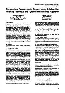
CI v a  1  H v a .....................................................................................................................................(10) This CI is used as a parameter in our approach to decide which set of predictions to allow going through and which set of predictions to hold back. Thus it is important to note that this parameter has no role to play in the prediction accuracy of an individual rating prediction but definitely has a role in altering the mean absolute error (MAE) and the root mean squared error (RMSE) of the recommender system as a whole. An appropriate choice of this parameter could cut off some potentially erroneous predictions and thereby improve the overall MAE and RMSE of the recommender system. However it is to be noted that with increasing threshold values of CI, more and more predictions would be held back thereby causing the coverage of the recommender system to monotonically decrease. Hence the threshold level for the parameter CI has to be chosen judiciously so as to obtain acceptable levels of overall prediction accuracy and coverage of the recommender system. The pseudocode for EBCF Algorithm is given in Appendix 6 and Appendix 7 while the notations used in the pseudocode are given in Appendix 5. 3.3. EBCF Recommender System The proposed architecture of the recommender system that incorporates the EBCF algorithm for predicting the unknown ratings is depicted in Figure 1. This system could provide recommendations to an active user of the system given some initial ratings of all users in the system. Preliminary computations such as the computation of the subjective probabilities (SP) of each of the rating levels of the active user corresponding to each of the rating levels of the prospective mentor as well as the computation of the predictability indices (PI) of each pair of users at each of the rating levels of the prospective mentor are done offline. The online operation begins when a user seeks a recommendation list from the system. The Entropy Based Collaborative Filtering Algorithm (EBCFA) is used to predict the ratings of the active user‟s unrated items. These unrated items are then ranked based upon the predicted value in decreasing order from which the top N items are presented to the user as a recommendation list. The pseudocode for producing a personalized recommendation list to a user seeking recommendation is shown in Appendix 8.

Page 221


User 1

User 2

User 3

User N

----------…

Supplying Initial data to the system Ratings database consisting of user id, item id, rating, time stamp etc

No of commonly rated items, SPs, PIs for each pair of users

Rescale ratings in the 1 to 5 range

Item

Item-User matrix User-User matrix

Offline Operation (done from time to time)

User

User

User

Select unrated items of user Select the set of fully qualified mentors for the user for each of the unrated items

Online Operation (done when a user seeks recommendation)

Predict the ratings of the unrated items using EBCFA Rank the unrated items based on the predicted ratings in decreasing order

User seeks recommendation

Top N items recommended to user

Figure 1: Architecture of the EBCF Recommender System 4.

Experiments and Results We tested our EBCF recommender system for prediction accuracy (accuracy in predicting the unknown ratings), classification accuracy (accuracy in classifying the good and bad items for each user) and novelty of recommendations (novelty as compared to the more obvious recommendations) on two benchmark datasets MovieLens1 and Jester2. MovieLens is a very sparse dataset containing 100,000 discrete ratings (1 to 5) from 943 users over 1682 movies. We sorted the entire MovieLens dataset by user id, grouped together all the ratings provided by the same 1 2

http://www.grouplens.org/ http://goldberg.berkeley.edu/jester-data/

Page 222


user and then created a training set-test set pair roughly in the ratio 80-20 (80-20 ratio is commonly used in such approaches). A random number (generated between 1 and 10 inclusive) helped in diverting a particular entry into the training set or test set. Thus we had 80,043 ratings in the training set and 19,957 ratings in the test set with roughly 80% of each user‟s ratings falling in the training set and roughly 20% of each user‟s ratings falling in the test set. Jester is a very dense dataset containing 4.1 million continuous ratings (-10.00 to +10.00) on 100 jokes from 73,421 users. These ratings are presented in three separate files: jester-data-1.zip, jester-data-2.zip, and jester-data3.zip. Due to our limited computational resources, we extracted a random sample (all the ratings of the first 1000 users in the file) from jester-data-1.zip that contains the ratings from 24,983 users who have rated 36 or more jokes. We expect that the results cannot be any worse than what is reported here when all the 73,421 users‟ ratings are used to test the approach owing to the general belief that collaborative filtering will only perform better with more learning data. Since the Jester dataset has continuous ratings in the range -10 to +10, we first rescale them in the range 1 to 5 (also in a continuous scale). We then split this data into a training set and test set with roughly 80% of each user‟s ratings in the training set and roughly 20% of each user‟s ratings in the test set. There were a total of 70,675 ratings in our sample provided by 1000 users over 100 jokes. After the training set test set split, there were 56,573 ratings in the training set and 14,102 ratings in the test set. 4.1. Prediction Accuracy Prediction accuracy metrics evaluate how good a recommender system is in correctly predicting the unknown ratings. Mean absolute error (MAE) gives the average of the absolute deviations of the predicted rating from the actual rating over all the predictions made. Root mean squared error (RMSE) gives the square root of the average of the squared errors over all the predictions made. RMSE places more emphasis on large errors that could lead to grossly wrong recommendations. When there is ratings sparsity, any prediction algorithm shall be capable of making rating predictions only for a certain percentage (measured by the coverage metric) of the test set. A good prediction algorithm would be the one that can demonstrate the lowest MAE, RMSE values coupled with the highest coverage value. Normalized mean absolute error (NMAE) facilitates performance comparison over different datasets that use different rating scales. MAE It is calculated as NMAE  ( MaximumRat ing  MinimumRat ing ) Prediction Accuracy for MovieLens dataset: The parameters that were to be set for our approach were the threshold levels for (1) the minimum required strength of a decision rule, (2) the minimum required commonly rated items between two users so as to become eligible to be the mentors of each other, (3) the minimum required PI at the appropriate rating level for a user to qualify as a mentor of the active user, (4) the CI that provides acceptable levels of accuracy and coverage. MovieLens dataset being a sparse one, we maintained the minimum required strength of a decision rule at 2. Several experiments were conducted to observe the sensitivity of each metric to each of the other three parameters at different training set/test set ratios. For the MovieLens dataset, when CI threshold was set to 0.0 i.e. when none of the predictions were held back, and when the training set/test ratio was 80-20, EBCFA performed optimally when the threshold levels for the minimum PI and the minimum required commonly rated items between two users were chosen as 0.35 and 18 respectively. At these levels, for the training set-test set pair we have created, we observed the MAE, RMSE and coverage at various threshold levels of CI. These results are reported in Table 3 and depicted through Figures 2, 3 and 4.

Page 223


Table 3: Sensitivity of Consensus Index to Prediction Accuracy Metrics – MovieLens Dataset CI 0 0.05 0.1 0.15 0.2 0.25 0.3 0.35

0.4

MAE

0.7318

0.7301

0.7253

0.7164

0.7064

0.6928

0.6803

0.6754

0.6876

NMAE

0.1829

0.1825

0.1813

0.1791

0.1766

0.1732

0.1701

0.1689

0.1719

RMSE

1.0373

1.0359

1.0315

1.0226

1.0124

0.9987

0.9882

0.9908

1.0341

Coverage

92.83%

92.43%

90.96%

88.18%

83.13%

74.97%

63.09%

45.08%

25.47%

Note: Training set test set ratio was roughly 80-20; Threshold for Minimum commonly rated items was 18; Threshold for Minimum PI was 0.35

0.74 0.72 E A M

0.7 0.68 0.66

0

5 .0 0

.1 0

5 .1 0

.2 0

5 .2 0

Consensus Index

Figure 2: MAE for MovieLens Data

Figure 3: RMSE for MovieLens Data

Figure 4: Coverage% for MovieLens Data

Page 224

.3 0

5 .3 0

.4 0

5 .4 0


Prediction Accuracy for Jester dataset: We first had to tune the parameters for this dataset and through several experiments where we varied these parameters, we found that the system performed optimally when the minimum number of commonly rated items was chosen as 5 and the minimum required predictability index was chosen as 0.5. The results of the experiments on the training set-test set pair we have created from Jester dataset are reported in Table 4 and depicted through Figures 5, 6 and 7. Table 4: Sensitivity of Consensus Index to Prediction Accuracy Metrics – Jester Dataset CI 0 0.05 0.1 0.15 0.2 0.25 0.3

0.35

0.4

MAE

0.7057

0.7029

0.6957

0.6804

0.6616

0.6405

0.6136

0.5871

0.5540

NMAE

0.1764

0.1757

0.1739

0.1701

0.1654

0.1601

0.1534

0.1468

0.1385

RMSE

0.9241

0.9214

0.9143

0.8995

0.8805

0.8602

0.8341

0.8084

0.7742

Coverage

100%

99.18%

97.06%

93.33%

87.39%

80.41%

71.81%

61.91%

51.09%

Note: Training set test set ratio was roughly 80-20; Threshold for Minimum commonly rated items was 5, Threshold for Minimum PI was 0.5

Figure 5: MAE for Jester Data

Figure 6: RMSE for Jester Data

Page 225


Figure 7: Coverage% for Jester Data Comparative Results: In order to truly compare the EBCF approach with traditional CF approaches, and demonstrate its capability to handle the ratings sparsity issue better than traditional CF approaches, we needed to conduct another set of experiments using EBCF algorithm and a base CF algorithm simultaneously on the same training set-test set pair. Pearson correlation based CF algorithm was chosen as the base algorithm (termed Traditional collaborative filtering (TCF) henceforth) for two reasons. Firstly, it is the most popular approach and is one of the best algorithms for collaborative filtering as reported in Herlocker et al. [1999]. Secondly, it is a neighborhood based, memory based CF approach as is EBCF. Among the two techniques correlation-thresholding and best-n-neighbors to determine how many neighbors to select for an active user, Herlocker et al. [1999] recommend the latter (best-n-neighbors) technique as it does not limit prediction coverage as does the former technique. In the case of EBCF too, placing threshold values on the number of commonly rated items, PI and CI does limit coverage as can be seen from Tables 3 and 4. On the other hand, selecting the best-n-neighbors (without setting thresholds in any of the parameters like the number of co-rated items, PI, CI) safeguards coverage. Thus we adopt the best-n-neighbors technique to comparatively evaluate EBCF and TCF. It was also observed in Herlocker et al. [1999] that incorporating a significance weighting of n/50 to devalue correlations that are based on smaller number of co-rated items provided a significant gain in prediction accuracy. Though our experiments with Jester dataset showed the contrary, we did observe some gain in prediction accuracy in the MovieLens dataset but at the cost of prediction coverage. In the case of TCF with significance weighting, coverage reduces because the predicted value falls below the lower cut off point (0.5) in more number of predictions due to the devaluations. We report results of the TCF approach with and without the significance weighting as well as the EBCF approach for both datasets. Table 5 shows the comparative values for the MovieLens dataset while Table 6 shows the comparative values for the Jester dataset. Figures 8 and 9 depict the results graphically for MovieLens dataset while Figures 10 and 11 depict the same for Jester dataset (TCF with significance weighting n/50 is not shown for Jester dataset as it is out of range of the shown graph). Jester dataset being a dense dataset, the coverage is 100% throughout for all the three approaches i.e., TCF with significance weighting n/50, TCF without significance weighting and EBCF. However EBCF has the lowest MAE and RMSE throughout in Jester data. As far as the sparse MovieLens dataset is concerned, EBCF has the largest coverage percentage (99.76%). TCF with significance weighting shows the lowest MAE and RMSE throughout in MovieLens data. But the coverage% for the same is only about 74.5%. If coverage as low as this is acceptable, then EBCF is capable of outperforming TCF with significance weighting too. As shown in Table 3, for EBCF, when the threshold for CI is set to 0.25, MAE =0.69282; RMSE=0.99873; Coverage%=74.97%. We believe this stands evidence to the fact that EBCF can cope with ratings sparsity better than traditional CF.

Page 226


Table 5: Comparative Results for Prediction Accuracy - MovieLens Dataset.

Best-N Neighbors

TCF No Significance weighting

MAE

RMSE

Coverage %

MAE

RMSE

0.7206 0.7129 0.7121 0.7127 0.7132 0.7135 0.7144 0.7150 0.7157 0.7161 0.7163 0.7163 0.7162 0.7161 0.7162 0.7162 0.7162 0.7162 0.7162 0.7162

1.0184 1.0094 1.0063 1.0060 1.0065 1.0065 1.0074 1.0076 1.0078 1.0080 1.0083 1.0082 1.0081 1.0080 1.0081 1.0081 1.0081 1.0081 1.0081 1.0081

74.43 74.47 74.44 74.45 74.45 74.45 74.45 74.45 74.45 74.45 74.45 74.45 74.45 74.45 74.45 74.45 74.45 74.45 74.45 74.45

0.8153 0.7704 0.7526 0.7396 0.7363 0.7325 0.7302 0.7312 0.7304 0.7312 0.7310 0.7304 0.7297 0.7301 0.7291 0.7285 0.7273 0.7276 0.7274 0.7275

1.1399 1.0844 1.0641 1.0488 1.0439 1.0405 1.0372 1.0385 1.0376 1.0364 1.0357 1.0353 1.0349 1.0352 1.0344 1.0335 1.0319 1.0320 1.0311 1.0318

Coverage %

96.78 97.77 98.28 98.33 98.38 98.51 98.64 98.61 98.67 98.73 98.69 98.70 98.72 98.72 98.74 98.76 98.77 98.75 98.74 98.72

EBCF MAE

RMSE

Coverage %

0.7460 0.7374 0.7321 0.7305 0.7296 0.7297 0.7286 0.7293 0.7299 0.7319 0.7327 0.7330 0.7334 0.7340 0.7339 0.7343 0.7345 0.7349 0.7356 0.7356

1.0617 1.0470 1.0374 1.0320 1.0291 1.0281 1.0264 1.0254 1.0247 1.0254 1.0256 1.0254 1.0248 1.0249 1.0246 1.0247 1.0248 1.0249 1.0252 1.0252

99.76 99.76 99.76 99.76 99.76 99.76 99.76 99.76 99.76 99.76 99.76 99.76 99.76 99.76 99.76 99.76 99.76 99.76 99.76 99.76

0.82 0.8 0.78 0.76 0.74 0.72 0.7

EBCF TCF No sig w t

19 0

17 0

15 0

13 0

11 0

90

70

50

TCF - sig w t n/50

30

10

MAE

10 20 30 40 50 60 70 80 90 100 110 120 130 140 150 160 170 180 190 200

TCF Significance weight - n/50

Best-N Neighbors

Figure 8: Comparative Results – MAE for MovieLens Dataset

1.1

EBCF

1.05

TCF No sig w t TCF sig w t n/50

1

19 0

17 0

15 0

13 0

11 0

90

70

50

30

0.95

10

RMSE

1.15

Best-N Neighbors

Figure 9: Comparative Results – RMSE for MovieLens Dataset

Page 227


Table 6: Comparative Results for Prediction Accuracy - Jester Dataset. TCF TCF Best-N Significance weight - n/50 No Significance weighting Neighbors MAE RMSE MAE RMSE 10 1.2074 1.5754 0.7751 20 1.1969 1.5671 0.7456 30 1.1908 1.5606 0.7344 40 1.1906 1.5607 0.7223 50 1.1922 1.5627 0.7216 60 1.1920 1.5618 0.7216 70 1.1920 1.5619 0.7190 80 1.1926 1.5624 0.7200 90 1.1924 1.5623 0.7175 100 1.1926 1.5625 0.7174 110 1.1932 1.5634 0.7183 120 1.1935 1.5633 0.7199 130 1.1938 1.5636 0.7175 140 1.1944 1.5644 0.7178 150 1.1949 1.5648 0.7173 160 1.1952 1.5652 0.7166 170 1.1949 1.5649 0.7174 180 1.1948 1.5646 0.7185 190 1.1946 1.5645 0.7187 200 1.1947 1.5646 0.7181 Note: Coverage % is 100% throughout for all the 3 approaches

1.0108 0.9727 0.9572 0.9383 0.9379 0.9374 0.9327 0.9357 0.9314 0.9304 0.9321 0.9352 0.9312 0.9314 0.9300 0.9288 0.9301 0.9320 0.9322 0.9308

EBCF MAE

RMSE

0.7282 0.7179 0.7141 0.7134 0.7128 0.7121 0.7118 0.7117 0.7116 0.7117 0.7119 0.7120 0.7121 0.7122 0.7125 0.7126 0.7129 0.7131 0.7132 0.7134

0.9665 0.9483 0.9405 0.9368 0.9342 0.9316 0.9301 0.9287 0.9272 0.9262 0.9254 0.9245 0.9238 0.9232 0.9228 0.9224 0.9220 0.9217 0.9213 0.9210

0.78

MAE

0.76 EBCF

0.74

TCF No sig wt

0.72 0.7 10 20 30 40 50 60 70 80 90 100 110 120 130 140 150 160 170 180 190 200 Best-N Neighbors

Figure 10: Comparative Results – MAE for Jester Dataset

1.02

RMSE

1 0.98

EBCF

0.96

TCF No sig wt

0.94 0.92 0.9 10 20 30 40 50 60 70 80 90 100 110 120 130 140 150 160 170 180 190 200 Best-N Neighbors

Figure 11: Comparative Results – RMSE for Jester Dataset

Page 228


4.2. Classification Accuracy Classification accuracy metrics evaluate the capability of a recommender system to correctly classify the good items (items having ratings above a certain threshold value and therefore considered relevant) and bad items for a user and recommend the good/relevant items alone to the user. The metrics used to evaluate classification accuracy are precision and recall. Precision is the probability of a selected item being relevant and recall is the probability of a relevant item being selected [Herlocker et al. 2004]. N N precision  rs and recall  rs where N r = Number of items relevant to the user; N s = number of items Nr

Ns

selected by the system as appropriate for recommendation to the user; N rs = Number of items both relevant to the user and selected by the system for recommending to the user. As the size of the recommendation list grows, precision would be adversely affected while recall would be positively affected. Hence the common practice is to observe the harmonic mean of precision and recall (known as the F1 metric) over varying recommendation list sizes. F1  2( precision )(recall ) ( precision )  ( recall )

When a recommender system produces a recommendation list of size N to a user, there would be no convincing way of determining whether an item selected by the recommender is also relevant to the user or not unless we have the rating of that user for that item in the test set. Hence it was observed in Herlocker et al. [2004] that precision and recall may be better approximated by restricting the recommendation list for a user to only those items for which the user‟s ratings are known and are present in the user‟s test set. Thus we adopt the same procedure for measuring precision and recall in all our experiments (in all approaches compared). We measure the precision and recall for each user for whom a recommendation list is possible to be produced by a particular approach and determine the average precision and average recall over all such users. We also calculate the F1 metric from these average values of precision and recall and present the same. Higher the F1 value better is the recommendation quality of the particular approach. Comparative Results: Besides TCF with and without significance weighting and EBCF, comparative experimentation to evaluate classification accuracy included one another simplistic approach where only the popular items are recommended to any user. Popular items are those that have been liked by a large number of users. Items that have an average rating of 3.5 or more and which have been rated by 10% or more number of users in the case of the sparse MovieLens data (30% or more number of users in the case of the denser Jester data) were termed popular items in our experiments. A related approach to find the popularity of items was used in Schickel & Faltings [2006]. MovieLens ratings being discrete, items with a rating greater than or equal to 4 were considered relevant. Jester ratings being continuous, items with a rating greater than or equal to 3.5 were considered relevant in our experiments. Table 7 and Figure 12 show the comparative results for MovieLens data while Table 8 and Figure 13 show the same for Jester data. As far as the F1 metric is concerned, on both datasets, the EBCF approach outperforms all the other approaches compared. Table 7: F1 Metric and Novelty for MovieLens Dataset – Comparative Results F1 Metric

Top N Recom

EBCF

TCF (sig wt n/50)

TCF (no sig wt)

1

0.811071

0.799479

2

0.796629

3 4 5 6

Novelty EBCF

TCF (sig wt n/50)

TCF (no sig wt)

0.764045

Popular item recom 0.794872

0.583634

0.481771

0.425843

0.806628

0.763741

0.76945

0.46631

0.394531

0.331461

0.789495

0.801389

0.753409

0.74364

0.42258

0.33507

0.288202

0.788901

0.785193

0.746279

0.73034

0.38207

0.301432

0.256554

0.781974

0.77318

0.741574

0.71591

0.3506

0.257422

0.24779

0.778519

0.763286

0.735949

0.70385

0.33219

0.234983

0.238858

7

0.774655

0.754528

0.732984

0.69737

0.32029

0.223884

0.237191

8

0.776655

0.753605

0.731469

0.69091

0.3139

0.213886

0.233191

9

0.773619

0.744641

0.728876

0.68604

0.30116

0.201433

0.228533

10

0.77093

0.739552

0.7246

0.6813

0.29409

0.200269

0.224154

11

0.76873

0.734463

0.723277

0.67679

0.28834

0.194185

0.224479

12

0.768183

0.730363

0.721007

0.67261

0.2835

0.191508

0.222767

Page 229


F1 Metric

0.85 EBCF

0.8

TCF sig w t n/50

0.75

TCF No sig w t 0.7

Popular Items Recommendation

0.65 1

2

3

4

5

6

7

8

9

10

11

12

Top-N Recom m endations

Figure 12: Comparative Results – F1 Metric for MovieLens Dataset Table 8: F1 Metric and Novelty for Jester Dataset – Comparative Results F1 Metric Top N Recom

Novelty

TCF (sig wt Popular item TCF (no sig wt) n/50) recom

EBCF

EBCF

TCF (sig wt n/50)

TCF (no sig wt)

1

0.832589

0.740286

0.734228

0.649789

0.453125

0.382413

0.302013

2

0.826285

0.697655

0.71324

0.616719

0.388393

0.297546

0.24094

3

0.79699

0.658071

0.686522

0.573482

0.361979

0.264145

0.233781

4

0.780949

0.648789

0.668267

0.528444

0.381138

0.285617

0.257047

5

0.76319

0.627527

0.656703

0.494474

0.392336

0.298193

0.281073

6

0.755902

0.609544

0.647424

0.4684

0.411533

0.30668

0.297897

7

0.753584

0.598799

0.637736

0.449137

0.425595

0.316321

0.308827

8

0.750317

0.590413

0.63325

0.436235

0.43548

0.325377

0.319422

9

0.75065

0.585953

0.631026

0.427627

0.444161

0.332904

0.327009

10

0.752097

0.582831

0.628845

0.42186

0.449692

0.337744

0.331498

11

0.752391

0.579663

0.626243

0.418005

0.45093

0.340458

0.332914

12

0.752354

0.577668

0.624183

0.415439

0.450676

0.342519

0.334022

F1 Metric

0.9 0.8

EBCF

0.7

TCF No sig w t

0.6

TCF sig w t n/50

0.5

Popular Items Recommendation

0.4 1

2

3

4

5

6

7

8

9

10

11

12

Top-N Recom m endations

Figure 13: Comparative Results – F1 Metric for Jester Dataset

Page 230


4.3. Metrics beyond accuracy Novelty evaluates the capability of a recommender system to recommend non-obvious items to a user [Herlocker et al. 2004]. We shall assume that obvious recommendations would come from a system that recommends to a user all popular items that the user has not yet seen. Then all those items that are liked by the user and found in the recommendation list produced by a particular approach and simultaneously not found in the recommendation list produced by the popular items recommendation approach may be deemed non obvious recommendations or novel recommendations. If a particular recommendation approach produces a recommendation list of size N and if R number of items in this list are relevant to the user but do not appear in the popular items recommendation list for the same user, then Novelty demonstrated by this approach for this user is given as Novelty  R . N A similar method to estimate novelty was already adopted in Schickel & Faltings [2006]. For each of the approaches (TCF with n/50 significance weighting, TCF without significance weighting and EBCF) we estimate the novelty of recommendations for all the users for whom the approach is able to generate a recommendation list and report the average value. Table 7 and Figure 14 show the comparative results (over varying recommendation list sizes) for MovieLens data while Table 8 and Figure 15 show the same for Jester data. With regard to the novelty metric, again it is EBCF that outperforms all the other approaches compared here on both the datasets.

0.6

Novelty

0.5

EBCF

0.4

TCF sig wt n/50

0.3

TCF No sig wt

0.2 0.1 1

2

3

4

5

6

7

8

9

10

11

12

Top-N Recommendations

Figure 14: Comparative Results – Novelty for MovieLens Dataset

0.5

Novelty

0.45 0.4

EBCF

0.35

TCF sig wt n/50 TCF No sig wt

0.3 0.25 0.2 1

2

3

4

5

6

7

8

9

10

11

12

Top-N Recommendations

Figure 15: Comparative Results – Novelty for Jester Dataset 4.4. Explaining the Recommendations Any recommender system will gain further credibility if it is capable of explaining its recommendations. EBCF recommender could easily explain every step leading to the final recommendations such as how mentors are picked for the active user, how the subjective opinion of each of the mentors is inferred from the co-rated items of the active user and the mentor, how these subjective opinions are aggregated to arrive at the probability of the active user providing each of the rating levels to the target item, how the target item‟s rating is predicted from these probabilities and finally how the predicted rating leads to the recommendation of the target item. This additional capability to come up with explanations for its recommendations will enhance the user‟s comfort level in accepting the personalized recommendations provided by the EBCF recommender system.

Page 231


5.

Limitations and Future Work While the EBCF approach seems to cope well with one of the issues of collaborative filtering i.e., ratings sparsity, it definitely is computationally more intensive than the TCF approach. While TCF computes one similarity value between each pair of users, EBCF computes 25 SPs and 5 PIs (for a 5 point rating scale) between each pair of users. Thus the memory requirement and response time of EBCF will be more than those of TCF. SP and PI calculations being offline operations, this drawback will affect only the offline operations to a greater extent in comparison to online operations. Considering the other merits of the proposed EBCF approach like better quality recommendations despite ratings sparsity, some tradeoff in terms of response time and memory requirement may be justified. Still, we acknowledge the need to devise means to reduce the response time drawback. Currently the time required by EBCF to make one rating prediction is in the order of milliseconds in the worst case (i.e. when the SP and PI values need to be extracted from external memory). The procedure for calculating SP and PI values as well as the procedure for generating personalized recommendation lists being conducive to parallel processing, one solution could be the deployment of multiple parallel processors. We plan to explore other means to address the response time drawback as part of future work. Following the footsteps of some of the hybrid approaches, as a part of our future endeavor, we would also like to examine the scope of blending EBCF with other public domain algorithms to further improve the recommendation quality. 6.

Conclusion We have proposed a neighborhood-based, memory-based collaborative filtering approach that embraces the notion of selective predictability and uses the information theoretic measure known as entropy to estimate the predictability between users at different rating levels. A recommender system architecture that makes rating predictions using the proposed entropy based collaborative filtering algorithm and offers personalized recommendation lists to users seeking recommendations is also presented. Comparative experiments reveal the potential of the proposed approach in dealing with the ratings sparsity issue better than traditional CF approaches. Besides, EBCF seems to outperform traditional CF approaches when tested over two popular datasets for Prediction Accuracy, as well as recommendation quality through classification accuracy and novelty of recommendations. The capability to explain its recommendations is one another feature leading to the credibility and congeniality of an EBCF recommender system. Thus EBCF seems to be a promising approach for product recommendation in real life e-commerce sites. Owing to its own merits, EBCF could very well play a significant role in ensemble models (for product recommendation) that seem to be the way forward. REFERENCES Adolphs, C. and A. Winkelmann, “Personalization Research in E-Commerce – A State of the Art Review (20002008),” Journal of Electronic Commerce Research, Vol. 11, No. 4: 326-341, 2010 Adomavicius, G. and A. Tuzhilin, “Toward the Next Generation of Recommender Systems: A Survey of the Stateof-the-Art and Possible Extensions,” IEEE Transactions on Knowledge and Data Engineering, Vol. 17, No. 6: 734-749, June 2005. Aggarwal, C.C., J.L. Wolf, K-L.Wu, and P.S. Yu, “Horting Hatches an Egg: A New Graph-Theoretic Approach to Collaborative Filtering,” Proceedings of the fifth ACM SIGKDD International Conference on Knowledge Discovery and Data Mining, pp. 201-212, 1999. Bell, R.M. and Y. Koren, “Improved Neighborhood-based Collaborative Filtering,” KDDCup’07, pp. 7-14, San Jose, California, USA, August 2007. Bell, R.M., Y. Koren, and C. Volinsky, “Modeling Relationships at Multiple Scales to Improve Accuracy of Large Recommender Systems,” Proc. 13th ACM SIGKDD International Conference on Knowledge Discovery and Data Mining, pp. 95-104, San Jose, California, USA, 2007. Breese, J.S., D. Heckerman, and C. Kadie, “Empirical Analysis of Predictive Algorithms for Collaborative Filtering,” Proceedings of Conference on Uncertainty in Artificial Intelligence, pp. 43-52, 1998 Cho, Y.H., J.K. Kim, and S.H. Kim, “A Personalized Recommender System Based on Web Usage Mining and Decision Tree Induction,” Expert Systems with Applications, Vol. 23, No. 3: 329-342, 2002 Delgado, J. and N. Ishii, “Memory-Based Weighted-Majority Prediction for Recommender Systems,” Proc. ACM SIGIR ’99 Workshop Recommender Systems: Algorithms and Evaluation, 1999. Desmarais-Frantz, A. and E. Aïmeur, “Community Cooperation in Recommender Systems,” Proceedings of the 2005 IEEE International Conference on e-Business Engineering (ICEBE’05), pp. 229-236, 2005

Page 232


Goldberg, D., D. Nichols, B.M. Oki, and D. Terry, “Using Collaborative Filtering to Weave an Information Tapestry,” Communications of ACM, Vol. 35, No. 12: 61-70, 1992. Herlocker, J.L., J.A. Konstan, A. Borchers, and J. Riedl, “An Algorithmic Framework for Performing Collaborative Filtering,” Proceedings of the 22nd Annual International ACM SIGIR Conference on Research and Development in Information Retrieval, pp. 230-237, Berkley, CA, USA, 1999. Herlocker, J.L., J.A. Konstan, L.G. Terveen, and J.T. Riedl, “Evaluating Collaborative Filtering Recommender Systems,” ACM Transactions on Information Systems, Vol. 22, No. 1: 5-53, 2004. Hill, W., L. Stead, M. Rosenstein, and G. Furnas, “Recommending and Evaluating Choices in a Virtual Community of Use,” Proceedings of ACM CHI ’95 Conference on Human Factors in Computing Systems, pp. 194-201, 1995. Huang, Z., D. Zeng, and H. Chen, “A Comparison of Collaborative Filtering Recommendation Algorithms for ECommerce,” IEEE Intelligent Systems, Vol. 22, No. 5: 68–78, 2007 Kim, J.K., Y.H. Cho, W.J. Kim, J.R. Kim, and J.H. Suh, “A Personalized Recommendation Procedure for Internet Shopping Support,” Electronic Commerce Research and Applications, Vol. 1, No. 3: 301-313, 2002. Koren, Y., “Factorization Meets the Neighborhood: a Multifaceted Collaborative Filtering Model,” Proceedings of the 14th ACM SIGKDD International Conference on Knowledge Discovery and Data Mining, pp. 426-434, 2008. Lee, W.P., C.H. Liu, and C.C. Lu, “Intelligent Agent-Based Systems for Personalized Recommendations in Internet Commerce,” Expert Systems with Applications, Vol. 22, No. 4: 275-284, 2002 Palanivel, K. and R. Sivakumar, “A Study on Implicit Feedback in Multicriteria E-Commerce Recommender System,” Journal of Electronic Commerce Research, Vol. 11, No. 2: 140-156, 2010 Resnick, P., N. Iakovou, M. Sushak, P. Bergstrom, and J. Riedl, “GroupLens: An Open Architecture for Collaborative Filtering of Netnews,” Proceedings of the 1994 Computer Supported Cooperative Work Conference, pp. 175-186, 1994. Sarwar, B., G. Karypis, J. Konstan, and J. Riedl, “Item-Based Collaborative Filtering Recommendation Algorithms,” Proceedings of the 10th International Conference on World Wide Web, pp. 285-295, Hong Kong, 2001. Schickel, V. and B. Faltings, “Inferring User‟s Preferences Using Ontologies,” Proceedings of AAAI, pp. 1413-1418, 2006 Schickel, V. and B. Faltings, “Using Hierarchical Clustering for Learning the Ontologies Used in Recommendation Systems,” Proceedings of International Conference on Knowledge Discovery and Data Mining, pp. 599-608, San Jose, California, USA, 2007. Shannon, C.E., “A Mathematical Theory of Communication,” Bell System Technical Journal, Vol. 27, pp. 379–423, 623–656, July, October, 1948. Shardanand, U. and P. Maes, “Social Information Filtering: Algorithms for Automating „Word of Mouth‟,” Proceedings of Conference on Human Factors in Computing Systems, pp. 210-217, ACM Press, 1995. Srikumar, K. and B. Bhasker, “Personalized Recommendations in E-Commerce,” International Journal of Electronic Business, Vol. 3, No. 1: 4-27, 2005 Yang, Y. and B. Padmanabhan, “Evaluation of Online Personalization Systems: A Survey of Evaluation Schemes and a Knowledge-Based Approach,” Journal of Electronic Commerce Research, Vol. 6, No. 2: 112-122, 2005

Page 233


Appendix 1 n

 SP(r )

x

1

ma

r 1

Proof [Case Yx > 0] n

n

Yx , r

r 1

r 1

Yx

 SP(r ) x ma  

1  n  1 Yx ,r   Yx   1   Yx  r 1  Yx



Proof [Case Yx = 0]

1 1  n   1 n r 1 n

n

n

 SP(r ) x ma   r 1

Appendix 2 | FQM v a | n

 P(r )

n

v



a

r 1

 ( PI

x

ma

 SP ( r ) x m  a )

m 1

| FQM v a |

 PI

r 1

x

ma

m 1

| FQM v a |





| FQM v a |

n

( PI

x

ma

m 1

  SP ( r )

x

ma

)

r 1



| FQM v a |

 PI

x

 ( PI

x

m 1

 1) 1

| FQM v a |

 PI

ma

ma

m 1

x

ma

m 1

Appendix 3 Sample PI calculation (using data in Table 2) Calculation of the Predictability Index of user a1 towards user a2 at the rating level 1 of a1: Step 1 Deriving the Decision Rule from the commonly rated items of a1 and a2 (Data in Table 2) “If user a1 rates an item as 1, then user a2 rates the same as 1 with SP of 0.8 ( SP(1) with SP of 0.2 ( SP(2) 0 ( SP (4)

1

a1 a2

1

a1 a2

 1 / 5  0.2) or as 3 with SP of 0 ( SP(3)

 0 / 5  0) or as 5 with SP of 0 ( SP(5)

1

a1 a2

1

a1 a2

1

a1 a2

 4 / 5  0.8) or as 2

 0 / 5  0) or as 4 with SP of

 0 / 5  0) ”

Step 2 Calculating Entropy at a1‟s level 1 5

H 1 a1  a2   SP (r ) 1 a1 a2  log 5 SP (r ) 1 a1 a2 r 1

 (0.8  log 5 0.8  0.2  log 5 0.2  0  log 5 0  0  log 5 0  0  log 5 0)  0.3109 [Note: SP ( r )

x

ma

* log n SP (r ) x ma is assumed to be 0 in Entropy calculations whenever SP (r ) x ma  0 ]

Step 3 Calculating the PI of user a1 towards user a2 at the rating level 1 of a1

Page 234


 (n  d )    (5  1)   0  f PI 1 a1  a2  (1  H 1 a1  a2 )  1    (1  0.3109)    1    0.6891  s  ( n  1)    (5  1)   2  2 Similarly, PI 5 a1 a3  0.290915 and PI a2 a1  0.5 Appendix 4 Sample calculations for Precision and Recall If a user‟s test set has the ratings of items „a‟, „b‟, „c‟, „d‟, „e‟, „f‟, „g‟, „h‟, „i‟, „j‟ and if items „a‟, „c‟, „d‟, „j‟ were rated above a threshold value (a rating greater than or equal to 4 on a 5 point scale) then N r  4 . When requested to produce a recommendation list of size 2 ( N s  2 ) if the system had selected items „a‟ and „d‟ then

N rs  2 . Precision= N rs / N s  2 / 2  1 . If the system had selected items „a‟ and „b‟ then precision = N rs / N s  1 / 2  0.5 . If the system had selected only item „a‟ (i.e.) if it had produced a recommendation list of size 1 only, then we calculate precision as Precision = N rs / N s  1 / 1  1 since it is only fair to say that the precision is 1 when the system recommends only the relevant items to the user irrespective of the recommendation list size it is capable of producing. When calculating recall, for the same example, where the system was requested to produce a recommendation list of size 2, if the system had selected items „a‟ and „d‟, we use the value of N r  2 and N rs  2 and calculate recall as recall = N rs / N r  2 / 2  1 . Here we take N r  2 and not 4 since we request the system to recommend only 2 items and hence there is no way for the system to pick out all the 4 items that are relevant to the user. It would be unfair to use N r  4 and say that the recall is only 0.5. If the system was requested to produce a recommendation list of size 4, then it could have in all possibility picked out all those 4 items showing the real recall value of 1. Appendix 5 Notations used in EBCFA X = set of all possible rating labels. For a 5 point rating scale as is assumed here, X = {1, 2, 3, 4, 5} A = set of all users in the system. |A| = N where N corresponds to the number of users in the system. PM a = set of all potential mentors of active user „a‟; PM a = A-{a};

PQM v a = set of all preliminarily qualified mentors of active user „a‟ for target item „v‟; FQM v a = set of all fully qualified mentors of active user „a‟ for target item „v‟;

H x ma = Entropy (H) of user „m‟ towards user „a‟ at the rating level „x‟ of „m‟; PI x ma = Predictability Index (PI) of user „m‟ towards user „a‟ at the rating level „x‟ of „m‟ ; SP(r ) x ma = Subjective Probability (SP) or the probability that the active user „a‟ will provide a rating „r‟ to the target item if the prospective mentor „m‟ had provided a rating „x‟ to the same target item;

P ( r ) v a = Overall Probability that the active user „a‟ will provide a rating „r‟ to the target item „v‟;

H v a = Entropy (H) of the five overall probabilities for the active user „a‟ for the target item „v‟; CI v a = Consensus Index of the mentors of an active user „a‟ for a target item „v‟.

Page 235


Appendix 6 Pseudocode to calculate the Predictability Indices (PI) and Subjective Probabilities (SP) Compute SP_PI (ratings matrix, minimum required strength of a rule) { For each user „a‟ in A { Set „a‟ as the active user PM a = A-{a} For each user „m‟ in PM a { Set „m‟ as the prospective mentor for „a‟ For each rating level „x‟ in X of „m‟ { For each rating level „r‟ in X of „a‟ {

SP (r ) x ma  SP (r ) x ma

Yx , r

ifYx  0 Yx 1  ifYx  0 n

} n

H x ma   SP(r ) x ma  log n SP(r ) x ma r 1

 (n  d )   f PI x ma  (1  H x ma )  1    s  (n  1)   } } } } Appendix 7 Pseudocode for computing predictions Compute Prediction (target item, active user, Minimum required PI, Minimum required number of commonly rated items between the prospective mentor and active user, Minimum required CI) { Set „a‟ as active user and „v‟ as target item

PM a = A-{a}; PQM v a   ; FQM v a   For each user „m‟ in PM a { If „m‟ has rated „v‟ then PQM

v

a

 PQM v a  m

} For each user ‟m‟ in PQM {

v

a

PI x ma > Minimum required PI and if „m‟ and „a‟ have commonly rated at least the v v Minimum required number of commonly rated items then FQM a  FQM a  m If }

Page 236


v

For each user ‟m‟ in FQM a { For each rating label „r‟ of „a‟ { Extract SP (r )

x

ma

where x corresponds to the rating provided by „m‟ to „v‟

} Extract

PI x ma where x corresponds to the rating provided by „m‟ to „v‟

} For each rating label „r‟ of „a‟ { v | FQM

P(r ) v a 

a|

 ( PI x ma  SP(r ) x ma ) m 1

| FQM v a |

 PI

x

ma

m 1

} n

H v a   P(r ) v a * log n P(r ) v a r 1

CI a  1  H v a v If CI a < Minimum required CI then hold back prediction v

If

CI v a > Minimum required CI then Rating estimation =

n

 P(r )

v

a

r

r 1

} Appendix 8 Pseudocode for making recommendations Recommend (active user, ratings matrix, user-user matrix comprising computed SPs and PIs) { For each item „v‟ in the set of items { If active user „a‟ has not rated the item { Call the function Compute Prediction If Prediction >= P  { Record the predicted value and add the item to the recommendation list } } } Rank the items in the recommendation list in decreasing order of predicted value Present the top N items to the active user as the recommendation list } Note: Items with a rating greater than or equal to some threshold value P  are considered relevant items

Page 237