PHYS 2912 Physics 2B (Advanced) ... everywhere, the School of Physics
addresses this by teaching the key topic areas a number of ..... A final property,
which.
PHYS 2012 Physics 2B PHYS 2912 Physics 2B (Advanced) Electromagnetic Properties of Matter Module 2009 Part 1 - Dielectric Materials Martijn de Sterke and B. James School of Physics, University of Sydney
Prologue In teaching physics we need to balance width and depth. In keeping with physics departments everywhere, the School of Physics addresses this by teaching the key topic areas a number of different times at increasing levels of sophistication. For example, our honours level course on Relativistic Quantum Mechanics is significantly more challenging than the first year Quantum Mechanics module you did last year. Of course this can only work because, you, the students, get more sophisticated over the years as well! After all you take more physics, maths and other courses, and so you think more about physics, and can start to make connections between different areas. The necessity for this is clear–by the time students do honours in 4th year, they need to carry out a research project, which typically involves acquiring new knowledge. In order to get to this level, you are exposed over the years to increasingly more fundamental descriptions of nature. The reason I am telling you this is that this semester is the next step in this increased level of difficulty and sophistication. The School of Physics considers the first three semesters of its program to be a broad-brush overview of a wide variety of subjects within physics. The treatment in this phase tends to be predominantly qualitative, with some numerical calculations. The second semester of second year is where we return to some of the topics and teach them at a deeper level, and this module on the Electromagnetic Properties of Matter is a prime example; after all, you already did electromagnetism last year. One of the key differences with the previous treatment is that we will be less qualitative. Mathematics is the language of physics, and in order to understand nature at an increasingly deep level we need to use it. We simply cannot solve our problems by staring at it long enough and coming up with the answer in that way. This was well summarized by E. Wigner in 1960 when he wrote about “The Unreasonable Effectiveness of Mathematics in the Natural Sciences.” In summary, these 19 lectures will be different than the previous lectures you have had–they are more quantitative and more mathematical, since ultimately that is how nature needs to be described.
1
1
Introduction
It is assumed that you are familiar with all the electromagnetic topics covered in first year physics. Strictly speaking these deal with electromagnetism in free space, but the presence of air makes minimal difference. In this module we will consider the subject of electromagnetism in the presence of materials, usually solids, the properties of which differ significantly from those of air. It is worth recalling two topics from last year: Gauss’s Law and the relationship between electric field and electric potential.
1.1
Gauss’s Law
Gauss’s Law is in the form of an integral. It tells us that the flux of electric field through a closed surface is proportional to the net charge inside the surface, with a constant of proportionality of 1/ε0 I Z qenclosed 1 E · dA = = dr ρ(r), (1) ε0 ε0 where ρ(r) is the charge density and the integration includes all space. The second equality expresses the fact that the integral over the charge density in the enclosed volume gives the total charge. This law is true only because the Coulomb force has an inverse square dependence. It applies to any closed surface, and to any distribution of charge. It can be used to determine expressions for the electric field produced by sufficiently symmetric charge distributions, such as the electric field due to: • a point charge, or any spherically symmetric charge distribution (charged spherical shell, uniformly charged sphere, etc.) • a line charge, or cylindrically symmetric charge distribution • an infinite sheet of charge Note that in the form in which it was given here, Gauss’ law can only deal with vacuum. We will see in Section 9 how this is generalized to dielectric media and how to deal with dielectric media more generally.
1.2
Electric field and electric potential
The effect of electric charge on the surrounding space can be described in terms of a vector field (electric field, E) or a scalar field (electric potential, V ). Obviously one must be related to the other. The potential difference between two points is given in terms of the electric field by Z
b
Vb − Va = −
E · dl
(2)
a
where the integral is independent of the path taken from point a to point b. Another way of stating the latter fact is that the line integral of the electric field around a closed loop is zero. The electrostatic field is therefore a conservative field. Of course if the integral did depend on the path taken then there would be little defining V in the first place.
2
The inverse relation gives us the component of the electric field in a particular direction. For example, the component of electric field in a direction specified by the coordinate l is El = −
∂V ∂l
(3)
where, for example, l could be the coordinates x, y, or z. We can write this as a single vector equation (in cartesian coordinates): µ E = (Ex , Ey , Ez ) = −
∂V ∂V ∂V , . ∂x ∂y ∂z
¶ ~ = −∇V
(4)
~ is the vector differential operator (called del or nabla): where ∇ ~ ≡ ( ∂ , ∂ , ∂ ). ∇ ∂x ∂y ∂z
(5)
This operator plays a central role in the differential formulation of the Maxwell equations. However, in this set of lectures we mostly, though not exclusively, deal with the integral formulation.
1.3
Differential form of Gauss’s law
Consider a volume element δxδyδz in a region of space with a volume charge density ρ. We apply Gauss’s law to this volume. Consider first the flux through the sides of the cube in the y − z plane, which is due to the electric field component Ex (see figure 1). If at x, the component is Ex then at x + δx it is Ex + (∂Ex /∂x)δx. The net outwards flux through the y − z sides of the volume element is therefore µ ¶ ∂Ex ∂Ex −Ex δyδz + Ex + δx δyδz = δxδyδz (6) ∂x ∂x z y
δz x
δx
Ex
Ex +
E
δy
∂E x δx ∂x
Figure 1: Electric field flux through a volume element Taking into account the other components, the total flux outwards through the volume element is ¶ µ ∂Ey ∂Ez ∂Ex + + δxδyδz (7) ∂x ∂y ∂z By Gauss’s law this equals the enclosed charge, which is ρδxδyδz, divided by ε0 . It follows µ ¶ ∂Ex ∂Ey ∂Ez ρ + + δxδyδz = δxδyδz (8) ∂x ∂y ∂z ε0 3
Thus, µ
∂Ex ∂Ey ∂Ez + + ∂x ∂y ∂z
¶ =
~ ·E = ∇
ρ ε0 ρ ε0
or
(9) (10)
~ ·E This is the differential form of Gauss’s law - it applies at any point in space. The quantity ∇ is called the divergence of the electric field. The differential equation embodies that fact that if there is positive (negative) charge density in a region there must be a net flux of field lines from (into) this region.
Interlude Before diving into the new material it is probably good to outline the main lines of argument in this part of the unit. Some of the items below may make little sense at this time, so I recommend that you look at these points while we progress through the notes. • Section 2: properties of dipoles. • Section 3: from a large distance, the field of an electrically neutral charge distribution is approximately that of a dipole. • Sections 4 and 5: Since neutral atoms can evidently be considered to be dipole-like, we consider the properties of a distribution of a large number of dipoles as a model for a dielectric medium (a medium without free charges). Having established the properties of a large collection of dipoles, we next need to work the magnitude of each of the individual dipoles. We do so in two steps. • Section 6: we establish the relation between the applied electric field and the dipole moment of an atom. • Section 7: the previous result lets us introduce a new field, the electric displacement, which is convenient for calculations. • Section 8: the last piece of the puzzle, namely the relation between the applied macroscopic field, and the field which an individual dipole notices. The two differ because inside the medium the field is affected by the presence of all the other dipoles. With the exception of Section 10, in which the energy associated with an electric field is calculated, the remaining chapters are applications and special cases of the general theory outlined above.
2 2.1
The electric dipole Electric field of a dipole
An electric dipole consists of two charges of equal magnitude but opposite sign (±q), separated by a distance d. The quantity p = qd is called the dipole moment. The dipole moment has a 4
vector representation p = qd, where the direction is from the negative to the positive charge, as shown in figure 2. Dipoles are key elements of electromagnetism, and are particularly important in the limit in which the observation point is much larger than the distance d. In this limit the electric fields, or the potential for that matter, of the positive and negative charges almost cancel. In fact the cancelation becomes better when the observation points moves further away. We will see the effect of this below. The reason we are interested in dipoles here is that they are at the basis of the model for dielectric materials that we use.
P y
x r-
r
θ
-q
r+
+q
p = qd Figure 2: Electric dipole At an arbitrary point, P, shown in figure 2, the electric field can be written as µ ¶ 1 q q E= r − r 3 + 3 − 4πε0 r+ r−
(11)
where r± = r ∓ d/2. We first consider two special cases:
Case 1: θ = 0
Ex
= = ≈
µ ¶ 1 q q − 4πε0 (r − d/2)2 (r + d/2)2 µ ¶ 2 q (r + d/2) − (r − d/2)2 4πε0 (r2 − d2 /4)2 1 2p 4πε0 r3
for r À d/2. Clearly Ey = 0.
5
(12) (13) (14)
Case 2: θ = π/2 Ex = −
µ
1 4πε0
where cos φ =
(r2
For r À d/2 this reduces to Ex = −
2q cos φ r2 + d2 /4
¶ (15)
d/2 + d2 /4)1/2
(16)
1 p 4πε0 r3
(17)
Again, clearly Ey = 0. The electric field pattern for an electric dipole, showing field lines and surface of equal potential, is shown in Fig. 3.
Figure 3: Electric field lines and cross-sectional view of equipotential surfaces for an electric dipole
2.2
Electric potential of a dipole
As we know from first year, getting the electric field, which is a vector quantity, is somewhat tedious. It is more convenient to calculate the electric potential, and the field through Eq. (4) The electric potential for an electric dipole is given by µ ¶ q q 1 − (18) V = 4πε0 r+ r−
6
where, if r À d/2, r+ r−
≈ ≈
r − d cos θ/2 r + d cos θ/2
(19) (20)
Using (r ± d cos θ/2)−1 = r−1 (1 ± d cos θ/2r)−1 ≈ r−1 (1 ∓ d cos θ/2r), we find V =
1 p cos θ , 4πε0 r2
(21)
1 p · ˆr , 4πε0 r2
(22)
which in terms of vectors can be written as V =
where rˆ is the unit vector pointing in the direction of r. This confirms our earlier discussion: quite generally, provided you are far enough away, the potential decreases as r−2 , i.e. faster than the potential of a single charge. The reason is that the positive and negative charge almost cancel each other, but not quite (they exactly cancel as d → 0, and that this cancelation improves when the observation point moves further away. Exercises 1. (advanced only) Starting from Eq. (22), show using (4) that, in vector notation, the electric field can be written as 1 3(p · r)r − r2 p E= (23) 4πε0 r5 Hint: This is done most easily by writing the second factor in Eq. (22) as (p · r)/r3 = (px x + py y + pz z)/r3 . 2. Using Eq. (23) show that at point (r, θ),
Er
=
Eθ
=
1 2p cos θ 4πε0 r3 1 p sin θ 4πε0 r3
(24) (25)
and then show that the magnitude of the electric field at (r, θ) is given by E=
1 pp 3 cos2 θ + 1 4πε0 r3
(26)
3. Show the results above for Er and Eθ reduce to the correct values for Ex and Ey for θ = 0, π/2.
2.3
Torque on a dipole
When an electric dipole is in a uniform electric field the charges experience forces of equal magnitude, but in opposite directions, as illustrated in Fig. 4. If the dipole moment vector p is
7
Figure 4: Schematic of a dipole in a uniform electric field. The two charges are subject to equal, opposite forces, leading to a torque. not parallel to E, the dipole experiences a torque; if the angle between p and E is θ the torque is given by (taking the centre of the dipole as origin) τ = qE × d cos θ/2 + qE × d cos θ/2 = qdE cos θ.
(27)
In terms of vectors the torque can be written as τ = p × E.
(28)
Note that the torque is a maximum when p ⊥ E, and is equal to zero when p k E. If a dipole is free to rotate it would oscillate about the θ = 0 position; if there is friction it settles down to an equilibrium orientation where p k E.
2.4
Potential energy of a dipole
Because of the torque which tends to align the dipole with the electric field, a dipole has potential energy associated with its orientation in an electric field. Starting with θ = 0, the work required to rotate the dipole to angle θ is given by µ ¶ d d U = 2qE − cos θ = pE − pE cos θ (29) 2 2 This expression assume that the potential energy is zero at θ = 0. It is customary, however, to take the potential energy to be zero at θ = π/2, in which case U = −pE cos θ, or in terms of vectors U = −p · E (30)
2.5
Calculating E from V for an electric dipole
Given the form of equation 21. it is natural to use polar coordinates. As incremental displacements in the r and θ coordinates are δr and rδθ respectively, the radial and azimuthal components of the electric field are given by Er Eθ
∂V 1 2p cos θ = ∂r 4πε0 r3 1 ∂V 1 p sin θ = − = r ∂θ 4πε0 r3 = −
(31) (32)
These results are consistent with the directly calculated cartesian components for θ = 0, π/2 which were derived in Section 2.1. 8
Case 1: θ = 0
Ex
=
Ey
=
1 2p 4πε0 r3 Eθ = 0 Er =
(33) (34)
Case 2: θ = π/2
3
Ex
= −Eθ = −
Ey
= Er = 0
1 p 4πε0 r3
(35) (36)
Charge multipoles–(advanced only, except the first paragraph)
You may ask why we even considered dipoles in the previous section. After all, it may not be clear where we can find equal and opposite charges that are close together. Now as it happens, and this is an idea that we develop over the coming sections, the way we model atoms in electromagnetism is like tiny dipoles–in essence what happens is that the applied electric field pulls the nucleus and the electrons in opposite directions, therefore creating a dipole. Therefore, any treatment of how electric fields affect matter, and matter affects electric fields, needs to rely on the properties of dipoles. This idea is further developed in Sections 4 and 5. The remainder of this section deals with an associated problem that can be skipped by Regular students. Let us now consider a charge distribution ρ(r), that is confined to some limited region of space close to r0 , but is otherwise arbitrary, and let us calculate the associated electric potential at the origin, which is far away from the charges. The exact result is Z 1 ρ(r) V = dr. (37) 4πε0 r Now write r = r0 + ∆r, and so V =
1 4πε0
Z d∆r
ρ(r0 + ∆r) , |r0 + ∆r|
(38)
where r0 is fixed and ∆r = (∆x, ∆y, ∆z is the vector pointing from r0 to r. We now make use of the knowledge that the charge distribution is close to r0 and that the observation point is far away. We do so by expanding the denominator in a Taylor series where δr is the small parameter. The first term of this series is 1/r0 and it corresponds to assuming that all charges are located at r0 . However, is often in physics that it is the second term that we are interested in. Let us therefore push this to the next order: µ ¶ 1 1 ∂(1/r) ∂(1/r) ∂(1/r) ¯¯ = + ∆x + ∆y + ∆z (39) ¯ 0 + ··· r0 + ∆r r0 ∂x ∂y ∂z r where the vertical bar at the end indicates that the function is to be evaluated at r0 . Now note that 1 ∂r x ∂ 1 =− 2 = − 3, (40) ∂x r r ∂x r 9
p where the last equality can be checked by writing r = x2 + y 2 + z 2 , doing the differentiation. We now substitute this into (39) and then find for V Z Z 1 ρ(r0 + ∆r) 1 ρ(r0 + ∆r) V = d∆r − d∆r ∆r · r0 + · · · , (41) 0 4πε0 r 4πε0 (r0 )3 where ∆r · r0 = x0 ∆x + y 0 ∆y + z 0 ∆z. This may look somewhat messy, but recall that r0 is a constant vector that can be taken out of the integral. The first integral in (41) then simply gives the total charge q in the distribution. The interpretation of the second integral is slight more complicated. Let us rewrite (41) first as Z 1 Q 1 1 0 V = − r · d∆r ρ(r0 + ∆r)∆r. (42) 4πε0 r0 4πε0 (r0 )3 Let us have a closer look at the second integral. As an example, let us take ρ(r0 +∆r) = Q[δ(r+ )− δ(r− )], where δ is the Dirac delta-function. This gives Q(r+ − r− ), i.e., the dipole moment of the distribution. Even if the distribution is more complicated, consisting of a continuous distribution of charge, the integral picks out the net dipole moment. For example, even if the total charge Q = 0, it may be that the positive charge occurs predominantly at large x, and the negative charge predominantly at small x. In this case the distribution has a net dipole moment pointing in the x direction. With this, then we write V as V =
1 Q 1 p·r + + ··· , 0 4πε0 r 4πε0 (r)3
(43)
where the sign of the second term has flipped since we take the vector r now as pointing from the charges to the observer. As discussed, the first term corresponds to the effect of the net charge in the distribution, and if it is nonzero then at large distances it is the dominant contribution to the potential. For a distribution for which the net charge vanishes, the next term, involving the dipole moment of the distribution, is the dominant one. For a distribution for which p vanishes as well, the next higher order term is a quadrupole term, which we briefly discuss below. At sufficiently large distances consecutive terms in the series become progressively smaller. A final property, which is not proven here, is the following: in general the value of the dipole moment p is depends on the position of the origin, except when the net charge Q = 0. As mentioned, an electric dipole is part of a multipole hierarchy, of which the first four are shown in Figure 5: • monopole: a single charge, for which the electric field varies as 1/r2 , and the electric potential varies as 1/r; • dipole: two separated charges of equal magnitude and opposite sign, for which at large distances, the electric field varies as 1/r3 , and the electric potential varies as 1/r2 ; • quadrupole: two separated equal and opposite dipoles, for which at large distances, the electric field varies as 1/r4 , and the electric potential varies as 1/r3 . We do not prove the spatial dependence of the field and potential here, but the argument is the same as that before: a quadrupole can be considered to be two dipole close together and with opposite orientation. Seen from a large distance the dipole almost cancel, but not quite, and this cancelation improves when the distance to the observer increases.
10
-
+
+ -
-
+
+
+ -
-
+ -
monopole
+
dipole
quadrupole
+ octopole
Figure 5: Illustration of the hierarchy of electric multipoles. • octopole: two separated equal and opposite quadrupoles, for which at large distances (by inference), the electric field varies as 1/r5 , and the electric potential varies as 1/r4 . The multipole concept provides a way of approximating the fields of an arbitrary charge distribution at large distances by a sum of successively higher order (and progressively smaller) terms. Thus the electric field magnitude and electric potential can be written as µ ¶ 1 A B C E = + 3 + 4 + ... (44) 4πε0 r2 r r µ 0 ¶ 1 A B0 C0 V = + 2 + 3 + ... (45) 4πε0 r r r The first term is the field due to a point R charge of magnitude equal to the net charge of the distribution: Σqi for point charges and ρdr0 for a continuous charge distribution. The conclusion from this section is that when we have an arbitrary charge distribution then at a large distance the dominant contribution to the potential or the field comes from the net charge. It leads to a 1/r dependence in the potential and 1/r2 in the field. If the charge distribution is such that there is no net charge, then the dominant contribution comes from the dipole moment of the charge distribution, leading to a 1/r2 dependence in the potential and 1/r3 in the field. If in turn the dipole moment also vanishes, then the dominant term comes from the quadrupole distribution of the charges, etc.
4
One dimensional treatment of dielectrics
In this section we apply the knowledge from Section 3 to the description of the response of a large number of atoms to an applied field. Here we consider dielectric media, media which do not have free charge carriers. It therefore applies to insulating materials such as glass or various crystalline materials, but not to semiconductors or metals. The latter will be discussed in subsequent parts of this Unit. Electric dipoles are interesting in their own right but are also essential for the understanding of dielectric media: we think about dielectric media as consisting of atoms. An applied field pulls the electrons and the nuclei in opposite directions (recall that F = qE) setting up a dipole. Note that the argument developed in Section 3 applies here. The net charge in a medium would be expected to vanish, and thus the next highest term is the dipole term even if the charge distribution is continuous. The dipole moment might not be very large since the effective separation between the positive and negative charges would be a fraction of the size of an atom, but that does not matter here. Since there are lots of atoms the total effect might be substantial. To see this effect 11
Figure 6: One-dimensional geometry that we are considering: a medium is modeled as set of dipoles, all pointing in the +x direction between a and b, with the observation point at x. in an elementary way we consider a one-dimensional geometry so that full-blown vector calculus is not needed. Before commencing with the one-dimensional treatment, a brief comment regarding the assumptions we are making here: we assume that the constituent molecules are non-polar, which means that in the absence of an applied electric field they have no dipole moment; in other words, they do not have a permanent dipole moment. Rather, the atoms or molecules are assumed to have no dipole moment in the absence of an electric field–the dipole moments are induced by the applied field by pulling the positive and negative charges apart. The dielectric properties of materials consisting of polar molecules is discussed in Sec. 12. Let us consider a dipole p at position x0 pointing in the positive direction, and an observer located at x, as illustrated in Fig. 6. The potential dV at x due to this dipole is given by µ ¶ 1 p 1 d 1 dV = = p , (46) 4πε0 (x − x0 )2 4πε0 dx0 x − x0 where, since the derivative is taken with respect to the source point x0 the usual − sign does not show. Now let us take a collection of dipoles on the x-axis located between a and b. The density of dipoles, i.e., the dipole moment per unit length is P (x0 ). Note that P is generally not a uniform function of position since the density of dipoles (atoms) or the dipole moment per dipole (atom) may vary. The total potential V at position x due to all dipoles is then Z b 1 1 d V (x) = dx0 . (47) P (x0 ) 0 4πε0 a dx x − x0 We integrate by parts to find · ¸b Z b 1 1 1 1 dP (x0 ) 0 0 V (x) = P (x ) − dx . 4πε0 x − x0 a 4πε0 a x − x0 dx0
(48)
Now this is an interesting result: in both terms the distance between the dipole and the observer enters the denominator linearly, reminiscent of the way the potential of a point source is calculated. Let us therefore look at the two terms more closely. If P was a uniform function then the second term would vanish and the first term would be the only one left. Its interpretation is quite easy. If P is uniform then in inside the “medium” the positive and negative charges cancel each other out. It is only at the edges where they do not: at x = a there is some bare negative charge, whereas at x = b there is some bare positive charge. The bare charges each lead to a contribution to the potential at the observation point, described by the first term in (48). As mentioned, if P is uniform then inside the contribution from the end points are the only contribution to the potential at x. In contrast if P is not uniform then the second term in (48) 12
leads to a contribution from the bulk of the “medium.” The precise form of this may be not be obvious but it is clear that it must depend on the derivative of P . Having made this interpretation we note that the contribution to the potential at x by the one-dimensional medium consisting of tiny dipoles can be written as Z b 1 σb (b) 1 σb (a) 1 ρb (x0 ) 0 V (x) = + + dx . (49) 4πε0 x − b 4πε0 x − a 4πε0 a x − x0 Here ρb = −dP/dx and σb = P sign(n), where sign(n) is the direction of the normal pointing out of the medium. The subscript b is short for “bound,” as discussed in the next paragraph. Now in a more general situation where we have free charges and also medium consisting of dipoles, the total potential is simply given by the sum of the contributions from the free charges and the bound charges associated with dipoles, and therefore associated with the response of the medium. The charges are “bound” in that are bound to atoms. This in contrast to free charges in conductors that can roam freely. In the presence of a medium the ρ in Gauss’ Law needs to include both types of charges. We return to this in Section 7. We note that σb and ρb essentially describe the same phenomenon, namely that a nonuniformity in the distribution of P leads to net charges. The expression for ρb picks out the nonuniformity within the medium, whereas σb is the obvious and large nonuniformity that occur at the edges of the medium! However, they describe the same physics. In drawing our previous conclusions we have been somewhat cavalier in that we only considered the effect of the bound charges at positions outside the one-dimensional medium. For the collection of dipoles to be truly equivalent to the effect of free charges we must also consider internal points. However, this is tricky, since the local potential would vary enormously. For example, close to an atom the magnitude of the electric potential would be expected to be very large, whereas further away it might be expected to be smaller. However, it can be shown that the conclusion we reached earlier is universally valid.
5
Three dimensional treatment of dielectrics
The argument in the previous section was somewhat contrived in that we considered a onedimensional geometry. The full three dimensional calculation proceeds similarly, except that the mathematics, which relies on vector calculus, is somewhat more complicated. However, the results are fully consistent with those in Section 4. In the three-dimensional case we deal with a small volume, rather than with an interval. First of all we now define the macroscopic polarization P to be dipole moment per unit volume, i.e., P = Np
(50)
where N is the density of dipoles. Having defined P, we then find that the results from full three-dimensional calculations are ~ · P; ρb = − ∇
σb = P · n ˆ,
(51)
both of which are immediate generalizations of the one-dimensional results. In the first of these the del operator (defined in Eq. (5)) describes three-dimensional variations of the polarization. In the second expression n ˆ is the normal pointing out of the volume which we are considering. A characteristic of both these expressions is that variations of Px in the y-direction, say, do not contribute to the bound charge. For the case of the surface density of bound charge it is obvious 13
why: the dipoles are oriented parallel to the surface which does not lead to an accumulation of net charge at the boundary. We can take this argument one step further. Let us suppose that, for whatever reason, P (x) depends on time. Then we may expect that the effect is similar to the effect of a current, in this case a “bound” current, since the associated charges remain bound to atoms, or a polarization current. It can be shown that the polarization current Jb is given by Jb =
∂P , ∂t
(52)
which, since P has units of C/m2 , has the expected units of A/m2 , and which needs to be added to possible currents associated with free charges. The polarization current can be somewhat understood as follows: consider a medium with an applied field that is turned on. As a consequence the atoms or molecules form small dipoles where there were none before. In thinking about this argument it is easiest to assume that the electrons are fixed by the crystal structure and that the nuclei move to setup the dipole moments. The movement of the positive charges clearly generates a current, the polarization current.
6
Response of atoms and molecules
In the previous section we started we the assumption that the dipole moment per unit volume P had some value, from which we then determined the bound charge density. In this section we deal with the first question: given some electric field E, what is P? This is not entirely straightforward since the field that is setup by one of the dipoles would be expected to affect the other dipoles as well. In other words, the externally applied field E may differ from the local field Eloc the dipoles see. The local field can be thought of as a combination of the applied field and an internally generated field due to the atomic dipoles. To lowest order one might expect that p = αEloc , (53) where α the polarizability, a property of the individual atoms or molecules, describes the ease with which the positive and negative charges can be pulled away from each other. The key point here is that p and Eloc are assumed to be proportional. E electron cloud
+ . d
Figure 7: Induced electric dipole in an atom in the presence of the local electric field. We can estimate the polarizability α for hydrogen as follows. Assume that the electron charge is uniformly spread with density ρ over a spherical volume of radius a. An external electric field 14
Eloc causes the centres of the positive and negative charges to be displaced by an amount d. If we assume that the electrons are fixed by the lattice in which the atom is located, then the nucleus moves by d. The distance d is determined by the condition that the external field Eloc balances the field by the electrons. The latter can be calculated using Gauss’ law. At a position d from the centre of a uniform charge distribution the field due to the electrons has a strength 4πd2 E =
4πρd3 , 3ε0
(54)
and so, since this field at equilibrium equals the external field Eloc Eloc =
Qd ρd p = = , 3ε0 4πε0 a3 4πε0 a3
(55)
where Q is the total negative charge of the distribution. Therefore we find for the polarizability α=
p = 4πε0 a3 , Eloc
(56)
which is the result we were after. Taking a ≈ 10−10 m, we find α/4πε0 ≈ 10−30 m3 . This compares with the measured value of 0.66 × 10⁻³⁰ m3 for hydrogen.
7
The electric displacement field D
From our studies we found that an distribution of dipoles leads to the presence of bound charges at the edges and at positions where the distribution is inhomogeneous. Now we also know that the electric field is associated with the presence of charges; the key point here is that the nature of the charges, whether free or bound, does not matter for the electric field. Thus in Gauss’ law, which is a direct consequence of Coulomb’s law, the total charges ρf + ρb needs to be used, i.e., I Z 1 E · dA = (ρf + ρb )dr, (57) ε0 where ρf and ρb are understood to include possible surface charges, or, in differential form, ~ · E = ρf + ρb . ∇ ε0
(58)
~ · P, we can rewrite this as Now since from (51) ρb = −∇ ~ · E = 1 ρf − 1 ∇ ~ · P. ∇ ε0 ε0
(59)
Now this is interesting: we have seen that E arises from free and bound charges, whereas P arises from bound charges only. The relation allows us to define a third field, a field that arises from free charges only. This field, the electric displacement D, is defined as
so that
D = ε0 E + P
(60)
~ · D = ρf ∇
(61)
15
Now we have gone through this argument using the differential form of Gauss’ law. The integral form, with which we are more familiar reads Z I D · dA = ρf dr (62) So, in summary, we have identified three fields, the electric field E, which arises from all charges, the polarization P which arises from the bound charges, and the electric displacement D, which arises from the free charges only. The three fields are related by Eq. (60).
8
Response of the medium
We now have collected a lot of puzzle pieces. We have identified three fields and their sources, and their relation (60). We also understand how the atoms and molecules that make up the medium respond to an external field. However, one of the key relations is still missing. In some sense it is easy to see where: Eq. (60) is a single relation between three fields and can be considered to define D, and even though we understand the microscopic response of atoms, we do not yet know the macroscopic response of a medium. Such relation, which define the electric properties of a medium, and which thus distinguish vacuum, from metal and water, say are called constitutive relations, since they refer to the constitution (the make-up) of a medium. The constitutive relation is the missing puzzle piece and we now set out to discuss it. Earlier we studied the microscopic response of single atoms and found that, to lowest order, p = αEloc according to Eq. (53). The most straightforward way to obtain a macroscopic response is to combine Eqs. (50) and (53), thereby ignoring the difference between the applied and the local field, to find P = N αE. (63) As we discussed, the difference between Eloc and E is the effect of the response of the dipoles to the external field. The difference between these two fields can be ignored for very dilute systems, particularly gases. However, for dense system this is simply not good enough. Now it can be shown that under some conditions Eloc ≈ E + P/(3ε0 ) (essentially by the method described in Appendix A). For more complicated situations a numerical calculation is required. However, in general we can say that Eloc = E + KP/ε0
(64)
where K is some positive constant. We now combine Eqs (53) and (64), and remember that P = N p to find the constitutive relation P=
Nα E ≡ ²0 χE 1 − (N αK/ε0 )
(65)
where χ is the susceptibility of the medium, the macroscopic version of the polarizability. This expression is consistent with our earlier arguments: the total, macroscopic polarization of volume is the sum of all the dipoles moments present in that volume. In a gas or other dilute medium, each dipole has the strength αE (assuming the dipoles are identical) and the total polarization is thus N αE. In a dense medium the dipoles interact with each other so that the direct proportionality no longer holds. This effect is described by the denominator of Eq. (65). It is common to use the constitutive relation between D and E, which, by combining (60) and (65) can be written as D = ²0 εr E, where ²r = 1 + χ (66) 16
material vacuum air (1 atm) teflon perspex glass neoprene quartz ethanol methanol water
εr 1.0 1.00059 2.1 3.4 5-10 6.7 4.3 28 33 80
Table 1: Dielectric constant values for a number of different media. which defines the dielectric constant εr ,1 and which is the constitutive relation we are after. The key aspect of this relation is that D and E are directly proportional to each other. The proportionality constant, which, apart from a factor ε0 , is the dielectric constant, can either be calculated using (65), or can simply be measured. Some values of the dielectric constant are given in Table 1. It should be stressed here that constitutive relation (66) (or, equivalently (65)), have a different status than the other equations that we have encountered. The others describe the universal behaviour of electric fields and how they interact with matter. In contrast, Eqs. (66) and (65) describe the response of a large but finite class of materials. Both are needed to do meaningful work. Later on in this part of the course we briefly discuss materials that have more complicated constitutive relation. Perhaps the analogy with mechanics is the most obvious, in that the equations in this section are the equivalent of Newton’s equation, and they have thus universal validity. The constitutive relations are somewhat like the relation F = −kx, which applies to ideal springs, but not to other objects.
8.1
Polarizability and dielectric constant
We found that for dense media Eq. (65) holds, with K a constant where K = 1/3 for the particular case of spherical molecules or atoms. By inverting this relation and by using (66) we find that ε0 εr − 1 3ε0 εr − 1 = (67) α= N Kεr + (1 − K) N εr + 2 where the second equality applies to the case of K = 1/3, which is applicable to spherical cavities. Equation (67) is the famous Clausius-Mossotti equation which relates the microscopic atomic/molecular polarizability to the macroscopic counterpart. If εr ≈ 1, then εr + 2 ≈ 3 it reduces to the dilute medium form, Eq. (63). In spite of its somewhat crude origins the ClausiusMossotti equation is quite widely valid when applied to gases and (non-polar) liquids. The simple theory however fails for crystalline solids where the dipole interaction is more complicated because of orientational effects. 1 In
some text books the symbol for the dielectric constant is κ or K. However, in the scientific literature the symbol εr is invariably used, and we use this convention here.
17
Examples 1. For nitrogen gas at one atmosphere and 0◦ C, N = 2.52 × 1025 m−3 , εr = 1.00058. Since the gas is dilute, both formulas give α/4πε0 = 1.83 × 10⁻³⁰ m3 . For comparison, the experimental value is 1.74 × 10⁻³⁰ m3 . 2. Suppose that in a sample of diamond, P = 8.0 × 10⁻⁶ C.m−2 . For diamond the atomic weight is 12, the atomic number is 6, and its density is 3.51 × 10³ kg.m−3 . The number density is given by 3.51 × 10³ N = = 1.76 × 1029 m−3 (68) 12 × 1.66 × 10−27 Therefore, P 8.0 × 10⁻⁶ p= = = 4.5 × 10⁻³⁵ Cm (69) N 1.76 × 1029 If p = qδ, where q = 6 × 1.6 × 10−19 C, δ = 4.7 × 10⁻¹⁷ m. Given that for diamond, εr = 5.5, the value for α given by the dilute formula, as expected, does agree with result obtained using the Clausius-Mossotti equation. α/4πε0 α/4πε0
9
= 0.81 × 10⁻³⁰ m3 = 2.03 × 10⁻³⁰ m3
(Clausius − Mossotti equation) (dilute formula)
(70) (71)
Gauss law in the presence dielectrics
Section 1.1 had a brief reminder of the use of Gauss’ law in vacuum. Let us now see how it is applied in the presence of dielectric media. To do this we need to remind ourselves that we have control over the free charges, but not over the bound charges, since they merely appear in response to the applied field. We therefore need to deal in the first instance with the electric displacement field D since its component normal to the surface does not depend on bound charges at all. So rather than Eq. (57) for E, we use Eq. (62) for D. As an example, let us consider a dielectric sphere of radius R and dielectric constant εr , with a (free) charge Q at its centre. Our challenge is to find the electric field E everywhere. To do this, we use Gauss’ law, which should be possible since the geometry has a high level of symmetry. Recall from the argument in the previous paragraph that we do not know the bound charges, only the free charges and so it is best to apply Eq. (62) for D. This is straightforward and we immediately find that Q D= rˆ, (72) 4πr2 where rˆ is the unit vector pointing in the r direction. Note that D is orthogonal to the surface and so here this field does not depend on the bound charges at all. Now we have found D it is easy to find E using Eq. (66). Thus, for r < R we have E=
Q rˆ, 4πε0 εr r2
while for r > R
(73)
Q rˆ. (74) 4πε0 r2 Though we have considered only a single example here, it shows quite generally how to approach problems involving dielectrics. E=
18
10
Energy density of the electromagnetic field
10.1
Energy density in vacuum
In this section we study the energy density of the electromagnetic field and how it affected by the presence of a dielectric medium. In a sense it is a generalization of the type of problems that we discussed at the end of the previous section. However, we first consider free charges only. We start with the following thought experiment: we have a set of M discrete charges Qj that initially are all at infinity. Because of this they are independent of each other and in this configuration we take the potential energy to be zero. M = 2: Let us first consider the case in which M = 2. We let the charges, which initially were at infinity, to have a finite mutual distance r12 . The way to envisage this is to assume that charge 1 is fixed2 and then to bring charge 2 slowly in from infinity. In this case the potential energy is Q1 Q2 W2 = . (75) 4πε0 r12 M = 3: Let us now bring in the third charge Q3 . Let charges Q1 and Q2 be fixed. Then the additional potential energy that is acquired is Q1 Q3 Q2 Q3 + . 4πε0 r13 4πε0 r23
(76)
Q1 Q2 Q1 Q3 Q2 Q3 + + . 4πε0 r12 4πε0 r13 4πε0 r23
(77)
W30 = and so the total potential energy is W3 =
Arbitrary M : From the previous simple cases we see that WM =
1 Qi Qj 1 1 Qi Qj ΣM = ΣM , 4πε0 i,j>i rij 2 4πε0 i,j6=i rij
(78)
where the conditions on the sum require j to be larger than i, and unequal to i, respectively, and where the factor 1/2 expresses the fact the each ij term has acquired an identical ji counterpart. Let us now carve out of this double sum the terms for which i = 1: µ ¶ Q1 Q2 Q3 Wi=1 = + + ··· . (79) 2 4πε0 r12 4πε0 r13 Here the expression in brackets represents the potential at Q1 due to the all other charges. Denoting this potential by V1 , this can be written as 1 Q1 V1 . (80) 2 Had we not taken i = 1 but any other, arbitrary value for i = l, say, then we would have found Ql Vl /2, where, again, Vl is the potential at charge l due to al other charges. Wi=1 =
We can now therefore write the total potential energy of the system as WM =
1 M Σ Qi Vi , 2 i=1
(81)
which is the result that we were after. 2 The
force that is needed to keep charge 1 fixed does not do any work and it therefore does not contribute to the potential energy.
19
We now found an expression for the potential energy of a set of discrete charges. However, this begs the following question: “how did those discrete charges come together in the first place?”, and “do we not count the potential energy associated with these charges?”. In fact, this latter potential energy is automatically included if we write the continuous analogue of Eq. (81) Z 1 W = V ρdr, (82) 2 where now the charges are taken to be continuously distributed and so all charge accumulation is included. In fact, it can be shown that while Eq. (81) can be positive or negative (which is easy to see when M = 2), below we see that Eq. (82) can never be negative. The difference is the large potential energy that is needed to bring microscopic charges together to form the macroscopic charges. To rewrite Eq. (82) in a more useful form we use the one-dimensional approach as we did earlier. To do this we write the equation as Z 1 W = V (x)ρ(x)dx. (83) 2 Now we know from Section 1.3 that in one dimension ρ = ε0 dE/dx, and we also know that E = −dV /dx and so we can write Z ε0 d2 V W =− V dx. (84) 2 dx2 We now integrate by parts and find W =−
· ¸ ¶2 Z µ ε0 dV ε0 dV V + dx. 2 dx 2 dx
(85)
The first term is evaluated at the edges of the interval that we are considering, provided that it contains all the charges. However, nothing stops us from making this interval larger and larger. All this time the magnitude of the integrand decreases as |x|−3 , and so the contribution from the first term is negligible. In the second term, which, by the way, is never negative, we replace dV /dx by −E to get the final result. Had we considered a full three-dimensional geometry then the analysis would have been essentially the same and we would have found Z ε0 W = E2 dr, (86) 2 and the electric energy density per unit volume is thus ε0 E2 /2. Let us finish with a brief comment on the approach taken in this section. We started by calculating the mechanical energy associated with bringing charges together from infinity. We then interpreted this mechanical energy as having been used to set up the associated electric field, and so the energy is thought of as residing in the field. This type of approach is similar to that in earlier E&M courses which usually start out with the force between two charges. The interpretation of this mechanical result is then to introduce an electric field through the relation F = qE, and so the mechanical result is seen as the interaction between a charge and a field.
10.2
Energy density in dielectrics
Now we have evaluated the energy density in vacuum let us now see how it is affected by the presence of a dielectric. Fortunately we have done most of the hard work so this is relatively 20
easy. In fact Eq. (82) is still valid except that we replace ρ, which previously was the only charge available, is replaced by ρf , the free charge. We think about this as again bringing the charges in from infinity, but the potential is now affected by the dielectric. Thus Z 1 W = V (x)ρf (x)dr. (87) 2 By the same argument as before, this can be rewritten in terms of the field, and we find Z 1 W = D · E dr, 2
(88)
which reverts to result (86) in the absence of the dielectric. The energy density per unit volume is thus ²0 ²r E · E D·D D·E = = , (89) 2 2 2²0 ²r where the last two equalities are only valid for the dielectric media that we have been dealing with until now.
11
Capacitors
We have developed a powerful machinery to deal with dielectric media. Let us now use this in the simple case of a parallel plate capacitor. Although it is our intention is to look at the effect of dielectric material between the capacitor plates, we begin by recalling the properties of a vacuum capacitor. For a parallel plate capacitor consisting of two plates of area A, separated by a distance d, one with a charge of +Q and the other −Q, the electric field between the plates is given by σ Q E= = (90) ε0 ε0 A The potential difference is given by Qd V = Ed = , (91) ε0 A from which we get the capacitance of the parallel plate capacitor C=
11.1
Q ε0 A = . V d
(92)
Dielectric-filled capacitor
Let us consider a capacitor that is filled with a dielectric with dielectric constant εr . There is a number of ways to deal with this problem, but, as in Section 9, it is probably easiest to realize that displacement field D is unaffected by the dielectric as its sources are free charges only. From Eq. (61), and the same mathematical argument as applied earlier to E, we note that D = σf . Therefore, since D = ε0 εr E, this can be written as E = σf /(ε0 εr ), and thus V =
σf d , ε0 εr
(93)
since the potential is by definition the integral over the electric field and not over the displacement field. We next introduce the total charge Q = σf A and so V =
Qd , ε0 εr A 21
(94)
and so the capacitance is
Q ε0 εr A = , (95) V d and thus the dielectric increase the capacitance by a factor εr . The physical reason for this can be seen in Fig. 8: in the capacitor the dielectric becomes polarized with positive bound surface charges appearing at the negatively charged capacitor plate, and vice versa. These bound charges set up a field that partly cancels the field due to the free charges, hence, for the same amount of free charge, the potential goes, down, and thus the capacitance goes up see (Fig. 9). C=
-Q
A - + - + - + - + - +
- + + - + + +Q - + + - + + - + d
Figure 8: Schematic of a dielectric-filled capacitor
E + + + + + + + + + +
P
-
A
δ Figure 9: Polarisation of the dielectric between the capacitor plates As a final calculation we determine the potential energy U of the capacitor. Since D = σf = Q/A we find from the last of (89) that Q2 d . (96) U= 2Aε0 εr Then using Eq. (95) we find that 1 U = CV 2 , (97) 2 which in fact is valid for any type of capacitor, not just for parallel plate capacitors. Too see R R this, briefly, we note that U = QdV = C V dV which gives the answer above. 22
Examples 1. Determine the capacitance of a parallel plate capacitor, with plates of area A and spacing d, if a slab of dielectric with dielectric constant εr and thickness x (< d) is adjacent to one of the plates. Using D makes this problem quite straightforward. Suppose the magnitude of the charge on each plate is Q; this is free charge and determines D which is given by D = σf =
Q A
(98)
It follows that the electric fields in the dielectric-free and dielectric-filled regions are respectively Q/ε0 A and Q/εr ε0 A. The potential difference between the plates is therefore µ ¶ Q Q x d−x V = (d − x) + x=Q + (99) ε0 A εr ε0 A ε0 A εr ε0 A With a little algebra we find Q C= = V
µ
d−x x + ε0 A εr ε0 A
¶−1 =
κε0 A x + εr (d − x)
(100)
Note that this result has the correct limits as x → 0 (no dielectric) and x → d (completely filled with dielectric). 2. Suppose a dielectric slab (εr = 2.50) is inserted between the plates of an electrically isolated charged capacitor, which has a vacuum capacitance of 100 pF capacitor and is charged to 100 V. Compare the energy stored before and after, and explain any difference. When the dielectric is inserted the capacitance increases by a factor εr to 250 pF. As the capacitor is electrically isolated, the charge on the plates remains unchanged, with a value of Q = CV = 100 × 10−12 × 100 = 1.00 × 10⁻⁸ C (101) As Q remains constant we use U = Q2 /2C to calculate the stored energy. Before insertion of the dielectric slab, U=
Q2 10−16 = = 5.00 × 10⁻⁷ 2C 2 × 100 × 10−12
J
(102)
When the dielectric is inserted C increases by a factor εr = 2.5, while as noted Q remains constant. The energy stored is therefore less by a factor of 2.5, i.e 2.00 × 10⁻⁷ J. What happened to the energy? It has been consumed doing work to draw in the dielectric slab. In the absence of friction the dielectric slab would accelerate into the capacitor, overshoot and oscillate back and forth. With friction it is drawn in and the excess energy dissipated as heat. 3. Repeat the above problem, this time with the voltage kept constant. The capacitance again increases by a factor εr , so the charge Q = CV increases from its initial value (1.00 × 10⁻⁸ C) to Q = 2.50 × 10⁻⁸ C. As V remains constant it is convenient to calculate the energy stored using U = 1/2CV 2 , which gives U=
250 × 10−12 × 104 1 CV 2 = = 1.25 × 10⁻⁶ 2 2 23
J
(103)
Thus the energy has increased from the initial value of 5.00 × 10⁻⁷ J to 1.25 × 10⁻⁶ J, i.e. by an amount of 7.50 × 10⁻⁷ J. Where does this energy come from? In this case, to keep V constant the capacitor must remain connected to a power supply, from which charge flows to bring the charge up to its new higher value. The energy transferred from the power supply is U = ∆Q V = 1.50 × 10−8 × 100 = 1.50 × 10⁻⁶ J (104) This is in fact twice the amount required by the capacitor, so again the dielectric slab is drawn into the capacitor.
12
Dielectric materials containing polar molecules
Molecules which have an intrinsic (i.e. permanent) dipole moment (such as water) are called polar molecules. In the absence of an electric field, such dipoles in a gas or liquid have random orientations due to thermal motion, and hence P = 0. If an electric field is applied the dipoles tend to align with the field, but thermal motion prevent complete alignment. In fact it is clear that the degree of alignment depends upon the relative values of the energy associated with the dipole in the electric field (∼ pE), where p is the intrinsic dipole moment, and the thermal energy (∼ kT ), i.e. upon the ratio pE/kT . The polarisation of the medium at temperature T is given by the Langevin equation (see Appendix C), shown in figure 10 µ µ ¶ ¶ pE 1 P = N p coth − (105) kT pE/kT If pE/kT ¿ 1, then
µ P → Np
pE 3kT
¶ (106)
while for pE/kT À 1, P → Np
(107)
i.e., the dipoles are completely aligned with the electric field.
12.1
Frequency dependence of polarisation
As induced dipole moments require displacement of electrons only, the dielectric constant of a material consisting of non-polar molecules remains constant to very high frequencies. Dielectric consisting of polar molecules can have large dielectric constants due to alignment of the intrinsic dipole moments. However as the frequency of the applied field is increased the dipoles cannot reorient quickly enough to follow the field. Thus with increasing frequency the dielectric constant falls to a value corresponding to induced polarisation due to displacement of electrons only. As water molecules have an intrinsic dipole moment, water provides a good example: at dc εr = 80, while at 600 THz (500 nm) εr = 1.77. The latter value characterises the response of water to visible light frequencies. We will see later when we discuss electromagnetic waves that refractive index and dielectric constant are related simply n=
√
εr
Thus at optical frequencies, the refractive index of water is 24
(108) √
1.77 = 1.33.
Polarisation, P/np
1
0.8
0.6
0.4
0.2
0
0
5
10
15
pE/kT
Figure 10: The Langevin equation. The dashed lines show the limiting behaviour for pE/kT ¿ 1 and pE/kT À 1.
13 13.1
Other dielectric behaviour Anisotropic dielectric media
In an isotropic material, for which all directions are equivalent, the vectors E, P and D are parallel, and ε, εr and χe are constants. We consider non-linear materials, for which the latter is not necessarily true, later. In an anisotropic material P and D is not necessarily parallel to E, nor to each other. In this case the constants ε, εr and χe become tensors. For example, instead of P = ε0 χe E, we have (neglecting for notational simplicity the subscript e for electric susceptibility)
Px χxx Py = ε0 χyx Pz χzx
χxy χyy χzy
χxz Ex χyz Ey χzz Ez
(109)
Thus the constant χ is replaced by a 3 × 3 matrix X, called in this physical context a 2nd rank tensor. Equation 109 can be written as P = ε0 XE Similarly, D = ε0 (1 + χe )E becomes Dx 1 + χxx Dy = ε0 χyx Dz χzx
χxy 1 + χyy χzy
(110)
χxz Ex χyz Ey 1 + χzz Ez
(111)
For particular materials some of the tensor elements may be zero. However, P and D and E are parallel to each other only is χij = 0 for i 6= j and the χii are all equal, i.e. the material is isotropic.
25
13.1.1
Nonlinear dielectric media
For a nonlinear material, P is a non-linear function of E: P = ε0 (χ(1) E + χ(2) EE + χ(3) EEE + . . .)
(112)
where we wrote EE since the square of a vector is not defined (of course the square of its modulus, a scalar, is well defined). For typical field χ1 E À χ2 E 2 À χ3 E 3 À · · · . Amongst many others things, transparent nonlinear dielectric materials are used to generate harmonics of intense light from lasers. To see this consider the χ(2) term in the expansion above. If the electric field varies as cos(ωt), then the nonlinear polarization associated with this field is proportional to cos2 (ωt) = [1 + cos(2ωt)]/2. Let us forger about the constant part here. Rather, the key observation is that even though the field has a frequency ω, the response of the medium P has a component that varies at 2ω.3 If an experiment is well designed, this can lead to efficient “frequency doubling.” For example, infrared light at 1064 nm from a pulsed Nd-YAG laser can be efficiently frequency doubled to green light at 532 nm with tens of % of efficiency using a suitable nonlinear crystal.
13.2
Piezoelectricity
Piezoelectric materials have the property that mechanical stress produces polarisation within the medium, resulting in an electric field in the medium and therefore a potential difference between opposite faces. Stress causes a small distortion of the crystal structure, which in certain materials can lead to a dipole moment. The inverse behaviour also occurs: the application of a potential difference produces stress and hence strain (fractional change in dimensions) of the sample. Thus piezoelectric materials can be used as electromechanical transducers to transform a force to a potential difference and conversely a potential difference to a dimension change. Examples of common piezoelectric materials include quartz (SiO2 ), barium titanate (BaTiO3 ) and lead zirconate titanate (PZT: ceramics with varying proportions of Pb, Zr and Ti). Applications of piezoelectric materials include: • Stress → potential difference: gas lighters, microphones • Potential difference → strain: nano-position controllers, speakers, alarms, scanning tunneling microscopes A particularly important application of quartz is as a circuit component for stabilisation of electronic oscillators (quartz oscillators). Because of its piezoelectricity the electrical oscillations can be locked to a mechanical resonance of the crystal. Examples include applications which require high stability electric oscillations, such as clocks and watches and the generation of clock frequencies in digital circuitry such as microprocessors, In critical applications the crystal mechanical resonance frequency is further stabilised within high tolerances by keeping its temperature constant. In general the direction of the induced polarisation (and hence induced electric field E) is not parallel to the stress T. The relation between these two vector quantities involves a tensor ( a 3 × 3 matrix). Thus E = eT (113) 3 This, by the way, is the hallmark of nonlinear effects. Recall that linear effects cannot change frequencies. Linear effects can affect different frequencies in different ways, but cannot generate frequencies that were not there before–only nonlinear effects can do so.
26
where e is the piezoelectric tensor. In expanded exx (Ex , Ey , Ez ) = eyx ezx
notation, exy eyy ezy
exz Tx eyz Ty ezz Tz
(114)
This, in general, one component of E depends on all components of T, for example, Ex = exx Tx + exy Ty + exz Tz
(115)
or in condensed notation Ei = eij Tj where i = x, y, z and repeated subscripts imply summation.
13.3
Ferroelectric and antiferroelectric materials
A ferroelectric crystal has a permanent polarisation, Thus even in the absence of an applied electric field the center of positive charge is displaced from the centre of negative charge. All ferroelectric materials are piezoelectric (e.g. BaTiO3 is ferroelectric), but not all piezoelectric materials are ferromagnetic (e.g. quartz). The behaviour of ferromagnetic materials parallels that of ferromagnetic materials (whence the name, despite the absence of iron), which will be covered in more detail later in this module. Antiferroelectric materials have neighbouring domains with opposite polarisation so that the nett polarisation is zero. When stress is applied the cancelation is destroyed resulting in a nett polarisation.
13.4
Electrets
These are materials which contain molecules with permanent dipole moments, and sufficiently low melting points (e.g. waxes) so that the dipoles can be aligned in the molten state, and the alignment frozen in when the material solidifies.
Appendices A
Electric field at the centre of a spherical cavity in a dielectric (advanced)
If there is a spherical cavity in a polarised dielectric there is bound surface charge on the surface ˆ . Recall that n is the outward pointing normal, i.e. the normal that of the cavity given by P · n points from the medium towards the air. In this particular case, therefore, n points into the sphere and the surface charge on the right-hand side of the sphere is thus positive, and that on the negative side is negative. The electric field at the centre can be calculated by first determining the field due to the bound surface charge on the ring surface element shown in figure 11. The electric field on the axis of a uniform ring of charge q, of radius r, on the axis at a distance d from the centre of the ring is given by E=
q cos θ 4πε0 r2
where
27
cos θ =
d r
(116)
-
+
-
P +
r
-
+
θ
+ +
-
+
-
+
Figure 11: Calculation of the electric field at the centre of a spherical cavity in a dielectric For the ring element shown we replace q by the bound surface charge density P cos θ multiplied by the surface area of the ring element, 2πr sin θ × rdθ. Thus the field at the centre due to the ring of bound charge is given by dE =
2πr sin θ × rdθ P cos θ cos θ P = cos2 θ sin θdθ 2 4πε0 r 2ε0
(117)
The resultant field at the centre of the sphere is obtained by integrating over θ = 0 → π: · ¸π Z π P P − cos3 θ P E= cos2 θ sin θ = = (118) 2ε 2ε 3 3ε 0 0 0 0 0
B
Derivation of the Clausius-Mossotti equation for a random medium (advanced)
The derivation of the Clausius-Mossotti equation is subtle and is based on an argument originally due to Lorentz. The aim of the exercise is determine the difference between the applied field and the field experienced by a particular dipole inside the medium. The two are likely to be different since the the each dipole is surrounded by other dipoles which are very close by, which have strong localized fields. Because of thermal effects, these strong field are likely to vary with time. So the first part in the argument is to average over position and over time so that the strong fields average out. The next step is to determine the average contribution of the surrounding dipoles. Here we use Lorentz’ argument: let us distinguish the dipoles which are far away from those which are close by. We will treat the former in some average sense, while the nearby dipoles need to be treated one-by one. In order to determine which dipoles are far away and which are close by we draw an imaginary sphere around the dipole of interest. The dipoles falling within the sphere are considered close by, while the other are considered far away. Of course the radius of the sphere has to be chosen appropriately, but that can be done. We now consider the dipoles which are close-by. According to one of the exercises in Section 2
28
the electric field of a dipole is given by E(r) =
1 3(p · r)r − |r|2 p 4πε0 r5
(119)
Let us now assume that we are dealing with a random medium such as a glass. The atoms can then be considered to be located at arbitrary positions. To get the field at our particular dipole, therefore, we need to average over all positions (the radius of the sphere needs to be chosen sufficiently large that it contains a sufficient number of atoms to make the averaging sensible. Let us start with determining the average x-component of the electric field from (119) À ¿ 1 3(px x + py y + pz z)x − |r|2 px hEx i = (120) 4πε0 r5 where the h·i indicates a spatial average. Let us look at the numerator 3(px hxxi + py hyxi + pz hzxi) − hr2 ipx .
(121)
Now the x and y positions of the atoms are uncorrelated, and thus hxyi = hxihyi, and since the positions are random hxi = hyi = 0. The xz term is dealt with in a similar way, but the xx term is not. This is easy to see: x2 is never negative, and so its average cannot vanish (of course it it not always zero either). So the numerator can be written as
But
3px hxxi − hr2 ipx .
(122)
hr2 i = hx2 + y 2 + z 2 i = hx2 i + hy 2 i + hz 2 i = 3hx2 i,
(123)
since x, y and z are equivalent directions. Therefore hEx i = 0, and the same is true for the other field components. We have thus found that for a medium where the atoms are located in random positions, the average contribution of the near by dipole averages to zero. It should be noted that the same conclusion is reached for many other situations, for example when the dipoles are located on a cubic grid. So the only contribution to the field comes from the dipoles which are located far away. However, we already now their contribution from Eq. (118): E = P/(3ε0 ), and this is the result we are after. This argument leaves a substantial number of untied knots. To name but one: if only the dipoles located far away contribute to the electric field, then surely the boundaries of the medium are important too. We disregard all these issue and simply make the point that the result we have found here is qualitatively correct. We should not take the factor 1/3 too seriously, but the general form of the result is correct.
C
Derivation of the Langevin equation (Advanced)
The dielectric consists of permanent dipoles which have a range of orientations determined by the Boltzmann distribution. Consider a dipole making an angle θ to the electric field, with an energy −pE cos θ. The proportion of dipoles with this energy is proportional to the solid angle dΩ = 2π sin θdθ. As the component of the dipole in the direction of the electric field is p cos θ, the polarisation per unit volume is given by Z P = A 2πp
µ
π
exp 0
−pE cos θ kT 29
¶ cos θ sin θdθ
(124)
where A is a constant obtained by noting that ¶ µ Z π −pE cos θ N = A 2π sin θdθ exp kT 0
(125)
where N is the density of dipoles. The first integral can be done by parts; the second is straightforward. The results are (where a = pE/kT ) µ ¶ 1 P = A 2πp (a(ea + e−a ) − (ea − e−a )) (126) a2 µ ¶ 1 (ea − e−a ) (127) N = A 2π a from which we find
µ P = N p coth
µ
pE kT
30
1 − pE/kT
¶ (128)