Physically-Consistent Sensor Fusion in Contact-Rich Behaviors. Kendall Lowreyâ , Svetoslav Kolevâ , Yuval Tassaâ , Tom Erezâ & Emo Todorovâ . Abstractâ We ...
Physically-Consistent Sensor Fusion in Contact-Rich Behaviors Kendall Lowrey† , Svetoslav Kolev† , Yuval Tassa† , Tom Erez† & Emo Todorov†
Abstract— We describe a computationally-expensive but very accurate approach to state estimation, which fuses any available sensor data with physical consistency priors. This is done by combining the advantages of recursive estimation and fixedlag smoothing: at each step we re-estimate the trajectory over a time window into the past, but also use a recursive prior obtained from the previous time step via internal simulation. We also incorporate a physics engine into the estimator, which makes it possible to adjust the state estimates so that the inferred contact interactions are consistent with the observed accelerations. The estimator can utilize contact sensors to improve accuracy, but even in the absence of such sensors it reasons correctly about contact forces. Estimation speed and accuracy are demonstrated on a 28-DOF humanoid robot (Darwin) in a walking task. Timing tests and leave-one-out cross-validation show that the proposed approach can be used in real-time and is substantially more accurate than the EKF, without any over-fitting.
I. INTRODUCTION Accurate real-time estimation of a robot’s state is essential for a feedback controller to accomplish its goals. Contactrich behaviors such as dynamic locomotion and dexterous manipulation require particularly accurate state estimation, not only in terms of kinematics but also contacts and contact forces. Indeed manipulation occurs when the robot exerts forces on its environment through contacts. Useful physical manipulation requires precise planning of deliberate contacts and graceful response to accidental contacts, much like how humans move in the world. However, contact phenomena are difficult to predict and even more difficult to plan through; the binary nature of contacts makes them altogether different from other physical effects. Even when contacts are correctly detected, estimation is required to reason about them and provide dynamically consistent state that can be used for robust control. The predominant strategy of robotic manipulation is through quasi-static movements and rigid grasping [1][2][3][4]. Similarly, the predominant strategy to robotic locomotion is quasi-static ZMP control. Richer manipulations and interactions can be achieved by understanding contacts and using them for deliberate force transfer and thus control. Forces are exerted on the environment through contact points; contacts and friction are therefore a critical component of successful control since the presence or absence of contact determines the feasibility of a proposed maneuver. Furthermore, contact forces are highly non-linear functions of robot configuration as tiny differences in a robot’s state can make or break contacts. In completely stiff This work was supported by the National Science Foundation. † University of Washington, Seattle, USA {klowrey,svetko,tassa,etom,todorov}@cs.washington.edu
Fig. 1: Left: Darwin robot. Right: Model of the robot. White spheres are PhaseSpace markers. Colored lines are traces of the markers during recorded walking sequence.
bodies, this nonlinearity introduces a discontinuity in the dynamical model of the system together with hard constraints of joint configuration space. The best way to gather information about the state of the contacts is via tactile sensors that measure force or pressure. Here the strong nonlinearity works in our favor. The signal from a tactile sensor is extremely informative regarding the contact state and the configuration. Indeed, the skin on human end-effectors (hands, feet, lips, tongue), is densely covered with touch sensors. Even with this large sensing organ, there is plenty of evidence that the brain uses multiple modalities to refine predictive models of its body and environment while using these models for movement [5]. This sensing and the associated processing is critical for contact based manipulation [6]. Much like the role of skin, a role of the estimator is to identify what are the actual contacts among potential contacts as the robot moves through its environment. Here we assume that we start with a rough of estimate of the robot’s state; it can come from a vision based system or IMU integration. Given a rough estimate, there is a potential contact between any two object within a certain spatial margin. This disambiguation is challenging because the difference between a potential contact versus actual contact is very small in joint space. In other words, contacts do not have a smooth observation model. Even when tactile sensors are present, there are often parts of the robot that lack them. A robotic arm will usually have tactile sensors only the fingertips, while the palm, forearm and elbows will not be covered. Since a
contact can significantly change the dynamical behavior of the system, a dynamical model can be used to disambiguate the system’s contact state. Any deviation from the expected behavior is a strong indication that a contact is present. Furthermore, dynamical models can use contact information to better predict the future trajectory. With a correct knowledge of contact state, a contact-aware forward dynamics simulator can predict the state of the system. Knowing how a system affects its environment along with the state of contacts can be turned into an inference mechanism [7]. In essence, by giving the estimator a proper understanding of the system dynamics, including the difficult nature of contacts, a better prediction can be made to allow for more successful control. For example, particle filters are one technique used to localize contact phenomena using tactile sensors [8], but as manipulation tasks become more complex, the number of required particles grows exponentially with the number of contacts. This problem can be represented in a principled way in a Bayesian framework, where the physical predictions of the model are used as a prior with sensor readings as observations. The most basic implementation of the Bayesian maximum likelihood optimization is the Extended Kalman Filter (EKF), where generative models of the dynamics and the observations are used to predict and correct an estimate of the system’s current state. The EKF algorithm uses a linear approximation of the dynamic and observation models and takes a single Gauss-Newton step [9] to update the posterior. Our approach is best understood by contrasting it with the EKF. There are two key differences: First, we employ multiple iterations to find the maximum of the Bayesian posterior, re-approximating the dynamics and observation models at each iteration while taking multiple Gauss-Newton steps. Second, while the EKF aims to estimate the system’s current state given the previous state, we maintain a representation of the system’s history over a fixed number of steps into the past to estimate the likelihood of the entire trajectory. This is known as fixed-lag smoothing, except here we combine it with recursive estimation and use a recursively-defined prior from the previous time step. Thus the system reconsiders its past estimate in light of the new observations. Our approach can thus be viewed as a strict superset of the EKF. The question then is, can the added computation be done in realtime and does it increase accuracy significantly. The answer is yes and yes, as we will see in the results section. A unique feature of our approach is that we use a physics engine (MuJoCo) as part of the estimation process. It is needed to provide a model of physical consistency, and obtain the necessary derivatives for optimization. As a result, the proposed estimator can give rise to advanced “reasoning” as follows. Suppose we observe (through vision) that a passive object is accelerating beyond what would be expected from gravity. This implies that some active object (i.e. the robot) must be touching it and applying contact force. But what if the present position estimate corresponds to a configuration where the robot is not touching the object? Clearly this estimate is wrong. So the estimator will correct
the configuration in a way that it remains close to the available position measurements but now the robot touches the object – at the nearest point where a contact can be created. It will further adjust the depth of the contact so that the inferred contact force (from inverse contact dynamics – see below) accounts for the observed acceleration. Of course the estimator does not go through this reasoning process explicitly; instead it simply optimizes the Bayesian posterior defined with respect to the physics model. To facilitate optimization in the presence of contacts, we allow small contact forces from a distance – so that the optimizer can detect a gradient which tells it that moving closer and eventually creating contact will be beneficial in terms of explaining all available sensor data. II. FRAMEWORK A. Definitions We consider a system composed of robots, moveable objects that the robots can interact with, and a static environment with certain geometry and contact properties. Define the following quantities: symbol n h t tE �t p(�t ) ut But τt qt vt xt = (qt ; vt ) yt ft pt (yt |xt , τt ) p¯(x) pˆ(x)
meaning number of DOFs time step duration discrete time index estimation horizon perturbation force prior over perturbations control vector force generated by ut applied force (�t + But ) generalized position generalized velocity system state sensor data contact force data likelihood estimation prior estimation posterior
The time window for trajectory estimation (or fixed-lag smoothing) at step t is [t − tE , t]. The vectors v, τ, Bu, � have dimensionality n, while q has dimensionality greater than n because it contains quaternions used to encode root orientations. Nevertheless we use qa − qb to denote an ndimensional displacement vector. Since different sensors can operate at different rates, the dimensionality of yt varies with t and so does the likelihood pt . The time step h corresponds to the fastest update rate, and we assume that all other time steps are multiples of h. The model also has constant parameters that include inertial properties, sensor mounting frames, contact properties, object geometry. In this paper we assume that these parameters have already been inferred through offline system identification, perhaps using our earlier method [10] which combined system identification and trajectory estimation. Here our focus is on physically-consistent real-time state estimation with respect
to a known model. The only parameters we will estimate here (using the EM algorithm) are the sensor noise covariances. We will use the framework of Bayesian inference. The key quantity is the data likelihood – which is a probability density over the sensor data space. The shape of this density depends on the (modality-specific) sensor noise models, while its mean is given by the corresponding generative models as follows: Sensor Type encoder contact sensor 3D marker force sensor IMU
Generative Model corresponding element of qt corresponding element of ft computed from qt via forward kinematics computed from (qt , vt , v˙ t ) via eRNE computed from (qt , vt , v˙ t ) via eRNE
eRNE refers to an extended recursive Newton-Euler method we have implemented, which computes not only the joint interaction forces but also the expected measurements from force sensors and IMUs mounted anywhere on the system. This is done by augmenting the standard RNE recursion with the necessary coordinate transformations. B. Inverse contact dynamics Key to the efficiency of the proposed method is the new contact model we recently developed [11]. It is an extension of our earlier work [12] where we showed how the standard LCP model of contact can be relaxed to obtain a convex optimization problem which still yields realistic contact dynamics. We also showed that the inverse contact dynamics are the solution to a related convex optimization problem. Previously both the forward and inverse problems were handled by an iterative solver. In our latest work [11] we found that the inverse problem can in fact be solved analytically, in time that scales linearly with the number of contacts. Furthermore the new method does not require computation or factorization of the generalized inertia matrix. It only requires forward kinematics, collision detection, RNE, and our new analytical formula – all of which are linear-time (except for collision detection which in principle can be slow, but in the problems we are studying it takes a small fraction of the CPU time). Armed with this new analytical machinery, we can now simplify trajectory optimization in the presence of contacts. This simplification applies both to dynamic motion planning and to physically-consistent estimation, although the focus of this paper is on the latter. The idea is to represent the trajectory as a sequence of positions zt = (qt−tE , . . . , qt ) and compute all other relevant quantities as functions of z. In this way we avoid redundancy in the representation and the need to impose equality constraints (except for underactuation which is imposed by the perturbation prior). The velocity and acceleration are based on finite-differencing the positions over time:
vt v˙ t
= (qt − qt−1 )/h = (qt+1 − 2qt + qt−1 )/h2
The analytical inverse dynamics developed in [11] then provide the mapping (qt , vt , v˙ t ) → (τt , ft ) Thus given a triple of positions (qt−1 , qt , qt+1 ) we can recover all relevant quantities at time t and define cost functions (log-likelihoods and log-priors) of these quantities. We will further impose a smoothness prior which depends on the difference between controls at consecutive time steps; this adds a cost term that depends on a quadruple of positions. C. Predictor-Corrector Trajectory-based estimation can be done in the Bayesian framework using the predictor-corrector approach as follows. The predictor maps the posterior at time t − 1 to a prior at time t: ut−1
pˆ(zt−1 |y−∞ , . . . , yt−1 ) −−−→ p¯(zt |y−∞ , . . . , yt−1 )
(1)
This mapping uses the known control signal ut−1 to simulate the forward dynamics, starting at the marginal of pˆ at xt−1 and adding noise from a stochastic dynamics model. We use Gaussian models of the trajectory probabilities so marginalization as well as shifting the time window is straightforward. The corrector is where almost all the processing time will be spent. Instead of just correcting xt in light of yt as is done in traditional recursive estimation, we will correct the trajectory estimate over the entire time window [t − tE , t] using all the data from that window. We will do so by applying multiple Gauss-Newton iterations per time step, in contrast with the Extended Kalman Filter which only applies one iteration. This will increase estimation accuracy at the expense of processing time; timing and accuracy statistics are presented below. D. Estimation We use maximum a posteriori (MAP) estimation over the entire time window. Using Bayes rule and the standard conditional independence properties, the mean of the posterior is found by minimizing − log pˆ(zt ) = const − log p¯(zt )− t−1 X
log pk (yk |qk , vk , v˙ k ) + log p(τk − Buk ) (2)
k=t−tE +1
The first term on the right is the log of a normalizing constant which does not affect the optimization. Then we have the usual prior followed by the likelihood. The last term enforces physics consistency and will play an important role here. It arises because any physical inconsistencies in the candidate trajectory zt are attributed to external perturbations �t = τk − Buk , whose prior probability p(�t ) must be taken into account. The sharper this prior is, the more physically consistent the estimates will become at the expense of accounting for sensor data. We may not want it to be too
right knee
left hip pitch 0
rad
rad
1
0.5
−0.5 −1
0
−1.5
accelerometer x
accelerometer z 20
m⋅ s−2
m⋅ s−2
5
0
−5
10
0
gyroscope x
gyroscope z 1
rad⋅ s−1
rad⋅ s−1
1
0
−1
0
−1
right heel impulse
left heel impulse 0.2
N⋅ s
N⋅ s
0.2
0.1
0
2.8
3
3.2
3.4
3.6
3.8
4
4.2
0.1
0
2.8
3
3.2
3.4
time (s)
3.6
3.8
4
4.2
time (s)
Fig. 2: Leave-one-out prediction test. Blue thick lines are the collected sensor measurements. Black dotted lines correspond to the estimate of that sensor using all available data. Red lines are the prediction of a sensor’s values when the sensor is unavailable to the estimator.
sharp, because physical consistency is assessed through the model which may be incorrect. Since we use Gaussian probability models, the minimization reduces to non-linear least squares: n 2 min kzt − z¯t kP + zt
t−1 X
2
kyk − y¯k (qk , vk , v˙ k )kS +
k=t−tE +1 2
k¯ τ (qk , vk , v˙ k ) − Buk kR
o
(3)
Here the functions y¯k , τ¯ denote the generative sensor model and the inverse dynamics respectively. The matrices P, S, R which appear in the weighted L2 norms are the inverse covariances of the corresponding Gaussian densities. The computationally-expensive phase is evaluating and linearizing the functions y¯k , τ¯. Once this is done, we have a (symmetric positive-definite) approximation to the Hessian of the cost function and can apply one step of the GaussNewton method, using the Levenberg-Marquardt procedure for (adaptive) linesearch. After convergence the Hessian is used to update the inverse covariance P . Because the cost function decomposes into a sum of costs over triples (or quadruples when using smoothing) of positions, the Hessian is band-diagonal. This allows very fast Cholesky decomposition without fill-in, implemented with our custom code.
E. Recursive Prior 2
The prior term kzt − z¯t kP in equation (2) is derived from the posterior of the last time step in a recursive fashion. The oldest measurement qt−tE is dropped and the gaussian is conditioned on its value. The first n elements of the mean are just truncated. The covariance is updated using ¯ t−t +1:t − the standard formula P −1 = Σt−tE +1:t = Σ E −1 ¯ T ¯ ¯ Σt−tE +1:t Σt−tE Σt−tE +1:t . Finally, a new configuration qt+1 is appended to the trajectory using the forward dynamics model, with a large diagonal covariance σIn corresponding to modeling error. As can be seen in the bottom left of Figure 4, the double inversion produces fill-in in P , but the additional terms are small. We have found that the simple approximation h¯ i P 0 P = t−tE +1:t −1 0
σ
In
which maintains sparsity (Figure 4, bottom left), does not perceptibly harm the convergence of the estimator. III. EXPERIMENTAL PLATFORM A. Hardware overview The data used to test our estimation algorithm was collected from a Darwin-OP robot produced by Robotis Ltd. The robot has 26 degrees-of-freedom: 3 positions, 3 orientations and 20 joints actuated with MX-28 servo-type motors. Joint encoders have 12-bit resolution, measuring discrete angles of 2π/4096 radians. An integrated IMU provides 3axis accelerometer and gyroscope readings and each foot is equipped with four pressure sensors at the corners. The
negative log−likelihood
0.05 tE = 1 0.04
tE = 3 tE = 15
0.03
tE = 30
0.02 0.01 0
1
2
3
4
5
Hessian
Hessian with 3rd−order term
Exact recursive prior
Approximate recursive prior
Gauss−Newton iterations 0
log−likelihood
−0.01 −0.02 tE = 1
−0.03
tE = 3 tE = 15
−0.04
tE = 30 −0.05
0
50
100
150
200
250
300
350
400
450
optimizations / second
Fig. 3: Performance of different window sizes and number of iterations. A window length of 1 and a single GaussNewton iteration corresponds to the EKF and is designated with a circle. Top: Negative log-likelihood as a function of iterations in the optimization step. Bottom: A Pareto-like curve taking into account the optimization time, we show log-likelihood as a function of optimization steps per second.
sensors are networked to a sub-controller ARM processor, which communicates to an x86 CPU over a USB to serial interface. B. Data Collection The data flow begins programmatically with querying a sub-controller for the desired data from sensors through a USB to serial interface. A feature of this robot is that all sensors and actuators are connected through the same halfduplex serial connection in a master-slave configuration. The subcontroller broadcasts a command for a given device based on a hard-coded ID across the network, and the appropriate device responds. This is repeated one by one for all sensors, and the returned data is aggregated for our use. This collected telemetry is then time-stamped and either cached to a file for offline analysis or streamed to an off-board computer. Data from the robot was collected at 125Hz. This rate was chosen to account for potential variability in reading the data off of the serial network while maintaining consistent timesteps between samples. Furthermore, this rate was also used to apply desired positions to the actuators; the control loop process consisted of taking a snapshot of data, calculating and applying controls, and then sleeping before waking every 8 milliseconds to begin again.
Fig. 4: Sparsity patterns. Top left: The Hessian (inverse covariance) of a trajectory with tE = 8 timesteps or 10 configurations q. Top right: Adding 3rd-order terms which penalize temporal variability of the applied controls. Bottom left: The matrix P of the exact recursive prior term 2 kzt − z¯t kP . Bottom right: The approximate recursive prior induces no additional fill-in to the original Hessian.
C. Phasespace An addition to the robot based sensors was our use of a PhaseSpace Impulse motion capture system. This system uses a network of high frame rate cameras tracking active LED trackers placed on the robot. The active LEDs were attached to the body of the Darwin-OP at known locations to give us accurate position data at 240Hz. The robot’s data and the PhaseSpace were both streamed to a networked computer that would combine the newest PhaseSpace sample with a sample from the robot as its data arrived. This was necessary as the robot’s telemetry occurred less frequently than the PhaseSpace system’s, but could still guarantee some synchronization between data streams. D. Behavior for Data Generation The controls that were supplied with the robot and used to generate complex movements. This included stepping in place, walking, and even falling and recovery. As we were intent on the design and validation of an estimator, this behavior was open loop control. The walking and stepping featured a ZMP-based cyclic pattern that could vary step length and foot placement angle, but did not receive feedback to adapt to changing state properties. Falling and recovery were scripts that could be played back when the robot’s inertial measurement unit detected a gravity vector sufficiently far from axis orthogonal to the ground plane. While simple in nature, these behaviors provided the base for rich sensor telemetry to challenge our estimator.
IV. RESULTS Figure 2 shows a snapshot of our results for the Darwin platform during walking. We left out sensor data, and let the estimator predict what the missing data should have been. The only sensor whose measurements are not well-predicted is the gyroscope, which we attribute to the small angular velocities of ∼ 1rad/sec, which do not have significant effect on the dynamics. Figure 3 shows the improvement of out method relative to the EKF, along with timing results. The “sweet-spot” appears to be 3 iterations with a window of 3 timesteps. V. FUTURE WORK The models we use recently developed optimization methods for both kinematic and dynamic system identification [10]. They will be applied here by attaching Vicon markers to the robots, sending diverse-yet-safe sequences of control signals, recording all available sensor data, and optimizing the model parameters. These parameters include link and armature inertias, joint friction and damping, control gains. We will also attach known masses to the robot and repeat the experiments, and then verify that the identification algorithm correctly interprets the change in dynamics.
Fig. 5: The Phantom-based manipulation platform. We plan to apply our estimation framework to a our manipulation system consisting of 4 Phantom Premium Haptic devices (Sensable Technologies). Here the contact state is of huge importance since we must actively make and break the contacts. While both the object and the Phantom robots themselves are instrumented with Vicon markers and the Phantom encoders have very high resolution, the fingertips currently lack tactile sensors making the contact estimation a very hard task. Complications arise from compliant nature
of the long linkage (including the 3D-printed fingertip) that makes it impossible to fully trust the joint encoders. R EFERENCES [1] A. Bicchi and V. Kumar, “Robotic grasping and contact: a review,” in IEEE International Conference on Robotics and Automation, 2000. Proceedings. ICRA ’00, vol. 1, 2000, pp. 348–353 vol.1. [2] Y. Wang and S. Boyd, “Fast model predictive control using online optimization,” IEEE Transactions on Control Systems Technology, vol. 18, no. 2, pp. 267–278, Mar. 2010. [3] A. Okamura, N. Smaby, and M. Cutkosky, “An overview of dexterous manipulation,” in IEEE International Conference on Robotics and Automation, 2000. Proceedings. ICRA ’00, vol. 1, 2000, pp. 255–262 vol.1. [4] C. Rosales, R. Suarez, M. Gabiccini, and A. Bicchi, “On the synthesis of feasible and prehensile robotic grasps,” in 2012 IEEE International Conference on Robotics and Automation (ICRA), May 2012, pp. 550– 556. [5] R. Shadmehr, The Computational Neurobiology of Reaching and Pointing: A Foundation for Motor Learning. MIT Press, 2005. [6] R. S. Johansson, “Sensory control of dexterous manipulation in humans,” Hand and brain: The neurophysiology and psychology of hand movements, vol. 1, p. 381414, 1996. [7] N. Kyriazis and A. Argyros, “Physically plausible 3D scene tracking: The single actor hypothesis,” in 2013 IEEE Conference on Computer Vision and Pattern Recognition, vol. 0. Los Alamitos, CA, USA: IEEE Computer Society, 2013, pp. 9–16. [8] M. Koval, M. Dogar, N. Pollard, and S. Srinivasa, “Pose estimation for contact manipulation with manifold particle filters,” in 2013 IEEE/RSJ International Conference on Intelligent Robots and Systems (IROS), Nov. 2013, pp. 4541–4548. [9] D. P. Bertsekas, “Incremental least squares methods and the extended kalman filter,” SIAM Journal on Optimization, vol. 6, no. 3, p. 807822, 1996. [10] T. Wu, Y. Tassa, V. Kumar, J. Movellan, and E. Todorov, “STAC: simultaneous tracking and calibration,” IEEE/RAS International Conference on Humanoid Robots (HUMANOIDS), 2013. [11] E. Todorov, “Analytically-invertible dynamics with contacts and constraints: Theory and implementation in MuJoCo,” in International Conference on Robotics and Automation (ICRA), 2014. [12] ——, “A convex, smooth and invertible contact model for trajectory optimization,” in International Conference on Robotics and Automation (ICRA). IEEE, May 2011, pp. 1071–1076.