Nov 20, 1997 - Measurements of the skylight polarized radiance distribution were performed at different measurement sites, atmospheric conditions, and three ...
Polarized radiance distribution measurement of skylight. II. Experiment and data Yi Liu and Kenneth Voss
Measurements of the skylight polarized radiance distribution were performed at different measurement sites, atmospheric conditions, and three wavelengths with our newly developed Polarization Radiance Distribution Camera System ~RADS-IIP!, an analyzer-type Stokes polarimeter. Three Stokes parameters of skylight ~I, Q, U!, the degree of polarization, and the plane of polarization are presented in image format. The Arago point and neutral lines have been observed with RADS-IIP. Qualitatively, the dependence of the intensity and polarization data on wavelength, solar zenith angle, and surface albedo is in agreement with the results from computations based on a plane-parallel Rayleigh atmospheric model. © 1997 Optical Society of America Key words: Stokes polarimeter, degree of polarization, neutral point, skylight.
1. Introduction
Polarization is an intrinsic property of the light field. Solar radiation as a natural light source is not polarized before it enters the atmosphere. The natural light field is polarized through scattering interactions1,2 with the atmospheric constituents, such as the permanent gases ~N2, O2, etc.!, gases with variable concentration ~O3, SO2, etc.!, and various solid and liquid particles ~aerosols, water, and ice crystals!. The pattern of skylight polarization3 is related to the Sun’s position, the distribution of various components of the atmosphere, and the underlying surface properties. Since the discovery of skylight polarization by Arago in 1809, observations of skylight polarization have been related to the studies of atmospheric turbidity4 – 6 and surface properties.7 The recent development of the Polarization Radiance Distribution Camera System8,9 ~RADS-IIP! offers a new method for observing skylight polarization and can provide the spectral polarized radiance distribution over the whole hemisphere quickly and accurately. It is generally recognized that the principal features of the brightness and polarization of the sunlit
Y. Liu is with Research and Data Systems Corporation, 7833 Walker Drive, Suite 550, Greenbelt, Maryland 20770. K. Voss is with the Department of Physics, University of Miami, P.O. Box 248046, Coral Gables, Florida 33124. Received 28 January 1997; revised manuscript received 30 June 1997. 0003-6935y97y338753-12$10.00y0 © 1997 Optical Society of America
sky can be explained in terms of Rayleigh scattering by molecules in the atmosphere.3 Modern radiative transfer theory in the investigation of polarization1,2,10 has been applied to studies on planetary atmospheres11,12 as well as the Earth–ocean system.13–15 Understanding the intensity and polarization of light in the atmosphere is also important in atmospheric correction of remotely sensed data. The atmospheric correction algorithm developed for Coastal Zone Color Scanner imagery16,17 is most easily understood first by consideration of only single scattering, including contributions arising from Rayleigh scattering and aerosol scattering. The analysis of multiple-scattering effects was based on scalar radiative transfer computations in model atmospheres.18 Recent advancements19,20 solved the exact ~vector! radiative transfer equation to compute the scalar radiance. Neglecting the polarization in radiance calculations in an atmosphere– ocean system introduces errors as large as 30%.21 Measurements of the total sky polarized radiance distribution can be used to test the validity of vector radiative transfer models. Through inversion techniques this distribution can also be used in the determination of physical and optical properties, such as the absorption and scattering phase function of aerosols,22 which cannot be done directly because of the difficulty in measuring the scattering phase function23 and the single-scattering albedo.24 2. Background
Although scattering in the real atmosphere is more complicated than Rayleigh scattering, knowledge of the intensity and polarization of light in a plane20 November 1997 y Vol. 36, No. 33 y APPLIED OPTICS
8753
Fig. 1. Normalized radiance on the principal plane with an azimuth angle of f 5 180° and a solar zenith angle of 53.1°. Radiance data are computed for a plane parallel Rayleigh atmospheric model with an underlying surface and then normalized to the solar constant; t and R represent optical depth and surface albedo, respectively. Data are shown for two optical depths, 0.05 and 0.25. Data for the Lambertian surface are from Coulson et al.11
parallel Rayleigh atmosphere is important for discussion of skylight. While quantitatively different, radiance distributions resulting from Rayleigh and Rayleighyaerosol conditions exhibit similar variation with Sun elevation, atmospheric turbidity, and other parameters.3 A.
Intensity of Skylight in a Model Atmosphere
To illustrate the dependence of the intensity of light in a model atmosphere on the surface properties, we performed computations using Gordon’s successive order approximation19 ~including polarization! in a Rayleigh atmosphere with a Fresnel reflecting surface at a Sun zenith angle of 53.1 and at optical depths of 0.05 and 0.25. Light intensities on the principal plane are shown in Fig. 1 and compared with results from Coulson et al.10 for the same atmosphere with a Lambertian reflecting surface. The surface reflectances R are displayed on the graph. As can be seen, a Fresnel surface increases the skylight intensity only slightly above a totally absorbing surface ~R 5 0!. A Lambertian surface reflectance of 0.25 affects the radiance distribution much more, as can be seen in our experimental data. In Fig. 1 the radiance was normalized to the solar constant. It can be seen that the normalized radiance increases as the reflectance increases owing to light’s being reflected from the surface. The normalized radiance also increases as the optical thickness increases. At this point it is worth noting that the separation between lines with different surface reflectances becomes larger as the optical thickness increases. Because the skylight radiance for a clear atmosphere is dependent on both atmospheric turbidity and surface albedo, it is useful to look at skylight measurements made at various geographic locations 8754
APPLIED OPTICS y Vol. 36, No. 33 y 20 November 1997
and times. We have chosen cases in which cloud interference was absent or minimum. B.
Polarization of Skylight in a Model Atmosphere
The principal interest in measurements of skylight polarization is its sensitivity to dust, haze, and pollution in the atmosphere.25,26 The maximum degree of polarization is diminished by the effects of aerosol scattering, and at the same time the neutral points ~Q 5 0, U 5 0, defined below! of the polarization field are shifted from their normal positions. To illustrate how the degree of polarization and its maximum vary with surface properties and optical thickness, we first look at computational results of a Rayleigh atmosphere, using the plane-parallel model.3 These changes are investigated with experimental data in Section 3. Figure 2 illustrates the degree of polarization in the principal plane ~azimuth angle 180° with a Sun zenith angle of 53.1°. The data were taken from the table computed by Coulson et al.11 It can be seen that the degree of polarization has a strong dependence on surface properties and optical thickness. As the surface reflectance or optical thickness increases, the degree of polarization decreases accordingly. The Fresnel reflecting surface case is not shown, as the degree of polarization over a Fresnel reflecting surface is only slightly larger than that over a totally absorbing surface. A convenient representation of the polarization of a light beam is the Stokes vector.2 The four components of this vector, labeled I, Q, U, and V, are defined in terms of the electric field.8,9 Simply, these may be defined as I 5 Il 1 Ir, U 5 I45 2 I135,
Q 5 Il 2 Ir, V 5 Irc 2 Ilc,
Fig. 2. Degree of polarization at various optical depths, from Coulson et al.11 Data are computed in the same atmosphere as in Fig. 1; t and R represent optical depth and surface albedo, respectively.
where Il is the intensity of light polarized in a reference plane; Ir is the intensity of light polarized perpendicular to this reference plane; I45 and I135 are the intensities of light polarized in planes 45° and 135° to the reference plane; and Irc and Ilc are the right and left circularly polarized light intensities. Other parameters used to describe the polarized light field are defined below. The linear degree of polarization is defined as ~Q2 1 U2!1y2yI. The importance of the Stokes parameters Q and U in the atmosphere is that they define the polarization state of the atmosphere. The neutral points are points where the degree of polarization is zero. Neutral points are then characterized by the double requirements Q 5 0 and U 5 0. For a Lambertian surface these requirements are only met simultaneously at points on the principal plane. The Arago point is located above the antisolar point. Two other points, the Babinet and Brewster points, are located above and below the Sun. Since, because of an occulter, the RADS-IIP instrument cannot measure the part of the sky in which the Babinet and Brewster points occur, we restrict our discussions to the Arago point. Neutral points can be outside the principal plane over a still water surface owing to Fresnel reflections from the air–water interface.27,28 Neutral points can also depart from their normal observed positions owing to light scattering by dust, haze, and other aerosols,25 which sug-
gests that neutral point positions are sensitive indicators of atmospheric turbidity.3 The lines that separate the regions of positive Q from the regions of negative Q are called neutral lines. Another parameter that can be deduced from the polarization field is the angle of the plane of polarization x, defined by U 5 Q tan~2x!, which is the angle between the plane of polarization and the vertical plane at the relevant azimuth. By symmetry, x must be 690° on the principal plane, depending on whether Q is positive or negative; in either case U 5 0. Also, when x is zero, U is zero. Neutral lines, lines of U 5 0, and the angle of the plane of polarization are particularly important to the examination of radiative transfer models. 3. Experiment and Data A.
Method of Measurement
Measurements of the polarization radiance distribution were all made with the RADS-IIP8,9 at the wavelengths 439, 560, and 667 nm. During normal operation the analyzer is placed at each of three polarizer positions, and an image is obtained. The resulting data images, plus a dark count image taken with the shutter closed, constitute the basic data of one measurement. The overall time period for one complete measurement is 2 min. After correction 20 November 1997 y Vol. 36, No. 33 y APPLIED OPTICS
8755
Fig. 4. Measurement site at the Science and Administration Building, RSMAS, used on 5 February 1996.
Fig. 3. AOD, measured with a shadowband radiometer, as a function of time, on 5 February and 12 February 1996.
for dark counts the three data images are analyzed, and values of the Stokes vectors are computed and saved in image format. The degree of polarization and angle of the plane of polarization can also be calculated and displayed in image format. Measurement errors arise from errors in the recorded light intensity and the calibrated Mueller matrix elements. The uncertainties in recorded light intensities are due to ~1! the measurements’ being taken in a series that extends ;1.5 min ~ideally measurements should be taken at the same time! and ~2! unavoidable stray light and noise in the optical and electronic system. Normally skylight does not change significantly in 1.5 min, especially when the Sun elevation is high. Stray light and noise have been accounted for to the best of our abilities, as shown in comparisons with other instruments.8 An analytical estimate shows that the error in determination of the Mueller matrix elements can reach a maximum of 2%. To minimize the blooming effect caused by the direct solar radiation and the limited dynamic range of the system, a Sun occulter was adopted in our system to block the direct solar radiation. This occulter also blocks a portion of the sky; as a result, a portion of the data is not available on all data images on the sun’s half of the atmosphere. B.
Description of Measurement Sites
The RADS-IIP polarimeter was deployed on top of the James L. Knight Physics Building on the main campus of the University of Miami on 12 February 1996 and on the top of the Science and Administration building at the Rosenstiel School of Marine and Atmospheric Sciences ~RSMAS! on 5 February 1996 ~at approximately 25°439 N and 80°169 W!. The aerosol optical depths ~AOD’s! for these days are shown in 8756
APPLIED OPTICS y Vol. 36, No. 33 y 20 November 1997
Fig. 3. The AOD measurements were made with a shadowband radiometer.29 It can be seen that AOD varies with wavelength and time. The day 12 February was very clear, and the surrounding area corresponds to a typical urban area. Buildings, vegetation, and surfaces of varied reflectances surround the site. Measurements taken on 5 February have different features ~Fig. 4!; southeast of the site is water, and northwest is land ~including buildings, vegetation, and land!. On that day there were clouds early in the morning and late in the afternoon, and clear sky conditions occurred between 10:00 a.m. and 2:00 p.m. C.
Radiance Distribution of Skylight
The data taken on 12 February are shown first. In these cases measurements of the sky radiance distribution were taken at three wavelengths ~439, 560, and 667 nm!; typical data are shown in contour plots. ~For brevity, only 439 and 667-nm data are shown. Figures 5~a!, 5~b!, and 5~c! are contour plots of the radiance distributions at 439 nm ~solar zenith angle 45.3°!, 667 nm ~solar zenith angle 47.2°!, and 439 nm ~solar zenith angle 77°!, respectively. In these images the center is the zenith direction, and the zenith angle is directly proportional to radius from the center. The concentric circles are at 30° and 60° zenith angles. The units are 1022 mWy~nm cm2 sr!. On the solar half of the hemisphere the rectangular area on the right side of the image is the Sun occulter used to block the direct solar radiation.8 In general, for all wavelengths, the minimum radiances appear on the antisolar half of the hemisphere. As the wavelength increases, the absolute value of the minimum region decreases. This reflects the wavelength dependence of Rayleigh scattering and explains the blue sky. It is important to note that the symmetry to the Sun’s principal plane exists in these images because of the approximately uniform reflectance background. One can also note the increase in radiance at the horizon due to the increased effective atmospheric path length at the horizon. As the Sun zenith angle increases, the absolute radiances de-
Fig. 5. Contour plots of skylight radiance @units 1022 mWy~nm cm2 sr!#. The data shown were taken on top of the James L. Knight Physics Building at the University of Miami on 12 February 1996. The origin of the coordinate shown corresponds to the zenith, and the inner and outer circles to 30° and 60° zenith angles, respectively. The rectangular area blocked by Sun occulter on the solar half of the hemisphere is left blank ~no data!. The black dot is the sun’s position. ~a! Measurement wavelength 439 nm, solar zenith angle 45.3°, AOD ~410 nm! 0.17; ~b! measurement wavelength 667 nm, solar zenith angle is 47.2°, AOD ~410 nm! is 0.20; ~c! measurement wavelength 439 nm, solar zenith angle 77°, AOD ~410 nm! 0.14.
crease at all wavelength bands, and the minimum regions shift with the Sun. Measurements were also performed on 5 February on top of the Science and Administration building at RSMAS to investigate the effect of surface inhomogeneities. The major features are similar to the 12 February data set. The area southeast of the measurement site at RSMAS is water, and to the northwest is land. A cold front passed through Miami immediately before 5 February, and the optical depths were higher than those on 12 February. Again, it was cloudy early in the morning and late in the afternoon. Skylight intensity was significantly higher as a result of higher optical depth. Figure 6~a! is a contour plot of light intensity at 439 nm
~solar zenith angle 46.3°!, and Fig. 6~b! is at 667 nm ~solar zenith angle 44.7°!. In Fig. 6~a! the minimum intensity regions are shifted toward the direction over the water and thus destroy the symmetry to the principal plane. This shift from the principal plane decreases as the wavelength increases and becomes invisible at 667 nm. The shift can be explained, since a Fresnel reflecting surface ~water! increases the skylight intensity only slightly, but a surface with R 5 0.25 ~approximates land! has a large effect ~Fig. 1!. D.
Stokes Parameter Q and Neutral Lines
Figure 7 shows the contour plots of the Stokes parameter Q for the images shown in Fig. 5. These 20 November 1997 y Vol. 36, No. 33 y APPLIED OPTICS
8757
ber 0! are formed clearly on the hemisphere opposite to the Sun. Parts of neutral lines are also formed on the Sun’s half of the atmosphere, but large parts of these lines have been blocked by the Sun occulter. The minimum Q ~negative number! appears on the principal plane, 90° from the solar position. Tables 1 and 2 list minimum values of Q on the principal plane. Q is negative inside the neutral lines but positive outside, and the maximum contours are symmetric to the principal plane and expand with the increasing solar zenith angle. As the solar zenith angle increases, neutral lines shrink significantly but still keep a similar shape and form a closed line. The contours crossing the principal plane seem to be dragged toward the zenith, and their shapes change significantly. The contour appears more jagged in Fig. 7~c! owing to decreased signal level at lower Sun elevation @same for Figs. 8~c! and 9~c!#. E.
Fig. 6. Contour plots of skylight radiance @units 1022 mWy~nm cm2 sr!#. The data shown were taken on top of the Science and Administration building at RSMAS ~Fig. 4! on 5 February 1996. The plots are prepared in the same way as in Fig. 5. ~a! Measurement wavelength 439 nm, solar zenith angle 46.3°, AOD ~410 nm! 0.35. Note that the radiance distribution is not symmetric to the principal plane owing to the inhomogenous underlying surface. The minimum region is shifted toward the direction over water. ~b! Measurement wavelength 667 nm, solar zenith angle 44.7°, AOD ~410 nm! 0.30.
plots demonstrate how Q changes with wavelength and Sun angle. The numbers shown on the graphs are first normalized to the intensity and multiplied by 1000. They all show good symmetry to the principal plane, as expected from a plane-parallel model and a uniform surface. The deviation from this symmetry appears mainly on the Sun’s half of the atmosphere. Neutral lines ~designated with num8758
APPLIED OPTICS y Vol. 36, No. 33 y 20 November 1997
Stokes Parameter U and Lines of U 5 0
Figure 8 shows the contour plots of the Stokes parameter U for the images shown in Fig. 5. These plots demonstrate the change in U with wavelength and Sun angle. The numbers shown on the graphs are first normalized to the intensity and multiplied by 1000. The Stokes parameter U is antisymmetric to the principal plane; U 5 0 lines appear only on the principal plane and on the Sun’s half of the atmosphere, which is in agreement with the computation results with a plane-parallel Rayleigh atmosphere model.3 In the contour plots, because the sky in the vicinity of the Sun has been blocked, closed U 5 0 lines are not shown, but the parts of lines shown suggest this trend. Again the deviation from antisymmetry seems to occur on the Sun’s side of the atmosphere. The maximum regions ~both negative and positive! occur on the half of the atmosphere opposite the Sun. As the solar zenith angle increases, these contours are displaced toward the zenith, and their shapes are deformed. As the wavelength increases, for constant solar zenith angle, the maximum region expands, which implies larger degrees of polarization at longer wavelength. Table 3 lists the maximum values of U. Note that when the Sun is low the U 5 0 line on the principal plane is deflected from a straight line and becomes a curve close to the horizon. This phenomenon is not seen in a Rayleigh-scattering plane-parallel model with a uniform surface. A possible explanation could be that water is southeast of the measurement site. As the Sun set ~west, azimuth angle ;247° from true north for the graphs shown!, the U 5 0 lines shifted toward the part of the atmosphere where the polarization is influenced by reflection from water. When the Sun was high, the water body was under the Sun’s half of the atmosphere and had a negligible effect. F.
Degree of Polarization and Neutral Points
Figure 9 shows the contour plots of the degree of polarization, P, for the images shown in Fig. 5.
Fig. 7. Contour plots of the Stokes parameter Q. Data shown are normalized to radiance and then multiplied by 1000. The plots are prepared in the same way as in Fig. 5, and the measurement descriptions for ~a!, ~b!, and ~c! correspond to Figs. 5~a!, 5~b!, and 5~c!, respectively. Neutral lines ~lines of Q 5 0! are designated by the number zero. At lower solar elevation ~c! contours are more jagged than those at higher solar elevation, ~a! and ~b!; the same is true for U ~Fig. 8! and P ~Fig. 9!. Note that Q is symmetric to the principal plane.
These plots demonstrate how P changes with wavelength and Sun angle. The numbers shown on the graphs were normalized to the radiances and then multiplied by a factor of 1000. The degree of polarization shows good symmetry to the principal plane. Starting from the position of the Sun ~Fig. 9!, the degree of polarization increases as the primary scattering angle increases. The maximum values occur
in the region where the primary scattering angle is 90° from the Sun, in agreement with our earlier discussion for a plane-parallel model. After the maximum region, the degree of polarization decreases as scattering angle increases. The maximum degree of polarization is larger for longer wavelengths. Because the Rayleigh optical thickness is smaller for longer wavelengths, light in the longer wavelengths
Table 1. Minimum QyI ~31000! on the Principal Plane as a Function of Solar Zenith Angle u0 at 439 nm
Table 2. Minimum QyI ~31000! on the Principal Plane
u0 40°
42.5°
44.5°
45.3°
52.6°
64.8°
69.3°
73.9°
77.1°
406
438
467
535
546
564
570
569
592
Wavelength
Solar Zenith Angle ~u0!
439 nm
560 nm
667 nm
45° 75°
2535 2592
2578 2646
2584 2638
20 November 1997 y Vol. 36, No. 33 y APPLIED OPTICS
8759
Fig. 8. Contour plot of the Stokes parameter U. Data shown are normalized to radiance and then multiplied by 1000. The plots are prepared in the same way as in Fig. 5, and the measurement descriptions for ~a!, ~b!, and ~c! correspond to Figs. 5~a!, 5~b!, and 5~c!, respectively. Lines of U 5 0 appears on the solar half of the atmosphere and on the principal plane. Note that U is antisymmetric to the principal plane.
suffers less multiple scattering and thus a larger maximum degree of polarization. Tables 4 and 5 lists maximum values of P on the principal plane. As in the real atmosphere, light interacts with aerosol particles as well as molecules; the degree of polarization deviates from the predictions of a simple Rayleigh atmosphere model. As Table 3. Maximum UyI ~31000!
Wavelength
Solar Zenith Angle ~u0!
439 nm
560 nm
667 nm
45° 75°
540 580
594 640
610 630
8760
APPLIED OPTICS y Vol. 36, No. 33 y 20 November 1997
the solar zenith angle increases, while the maximum degree of polarization moves with the Sun to maintain a scattering angle of 90°, new contours are formed around a point on the principal plane at which a minimum degree of polarization is shown. This point is the Arago point described below. As the solar zenith angle increases, the degree of polarization also increases for all three wavelengths in accord with theoretical expectations.11 Another feature of the contour plot at a lower Sun elevation is the deviation from symmetry; this could be caused by light reflected by the water and then scattered into the measurement site, compared with light reflected by land, as discussed above. In Fig. 10 we plot all Arago points observed at various Sun angles and at three wavelength bands.
Fig. 9. Contour plots of the degree of polarization P. Data shown are amplified by a factor of 1000. The plots are prepared in the same way as in Fig. 5, and the measurement descriptions for ~a!, ~b!, and ~c! correspond to Figs. 5~a!, 5~b!, and 5~c!, respectively. The maximum degree of polarization appears at 90° scattering angles. Note that P is symmetric to the principal plane.
Table 4. Maximum P ~31000! on the principal plane as a function of Solar-Zenith Angle u0 at 560 nm
u0 40°
41.8°
43.9°
46.4°
53.5°
66°
70.1°
74.5°
77°
494
468
460
578
624
630
647
633
646
Table 5. Maximum P ~31000! on the Principal Plane
Wavelength
Solar Zenith Angle ~u0!
439 nm
560 nm
667 nm
45° 75°
535 592
578 646
584 638
Fig. 10. Observed angular distance of the Arago point from the antisolar point versus solar elevation; data obtained on 12 February 1996. 20 November 1997 y Vol. 36, No. 33 y APPLIED OPTICS
8761
Fig. 11. Contour plots of angle of the plane of polarization x ~degrees!. Data shown are amplified by a factor of 100. The plots are prepared in the same way as in Fig. 5, and the measurement descriptions for ~a!, ~b!, and ~c! correspond to Figs. 5~a!, 5~b!, and 5~c!, respectively. These figures can be best understood by comparison with corresponding Q and U plots. Note that x is antisymmetric to the principal plane.
The positions of the neutral points are measured in angular distance from the antisolar point. It can be seen that this angular distance increases as the solar elevation increases. The observed neutral points are at larger angles than the positions computed for a Rayleigh atmosphere with a totally absorbing surface. In Fig. 10, the total optical depths are listed for each channel. The difference between the observed and computed values is due to light scattering by aerosols and surface reflections. G.
Plane of Polarization
Figure 11 shows contour plots of the angle of the plane of polarization, x ~in degrees! for the images shown in Fig. 5. The numbers shown on the graphs have been multiplied by a factor of 100. x is positive 8762
APPLIED OPTICS y Vol. 36, No. 33 y 20 November 1997
if the electric vector rotates counterclockwise away from the vertical plane and negative for the opposite. These contour plots can be best understood when compared with the corresponding Q and U plots shown in Figs. 7 and 8. First we point out that the heavily clustered lines on the principal plane are artifacts of the contour program. x is antisymmetric to the principal plane; thus on each side of the principal plane x approaches either 90° or 290°. The contour program sees an abrupt change of 180° when x crosses the principal plane and adds many lines close to the principal plane. x is 645° at the neutral lines and zero at lines of U 5 0, except in the principal plane. As the wavelength changes, x changes according to the changes of Q and U. As the Sun’s elevation decreases, the contour on the half of the
Table 6. Illustration of the Maximum Degree of Polarization ~u0 5 45°!a
Date, region
AOD at 410 nm
P at 439 nm
P at 560 nm
P at 667 nm
12 Feb., PP 5 Feb., PP 5 Feb., MP
0.20 0.35 0.35
535 301 400
578 355 456
584 420 510
a PP represents principal plane, MP represents the maximum P in the image.
change in the skylight distribution ~Figs. 6!. To illustrate how these factors affect the polarization, we choose contour plots of the degree of polarization at 439 nm @Fig. 12~a!# and 667 nm @Fig. 12~b!#. Though the region where the maximum degree of polarization occurs is 90° from the Sun in general, the maximum in the region most likely affected by water has higher values than the region most likely affected by land. This deviation from symmetry arises because the degree of polarization over a Fresnel reflecting surface is much higher than that over a Lambertian reflecting surface. As the wavelength increases, the degree of polarization also increases. Comparing Figs. 9~a! and 9~b! with Figs. 12~a! and 12~b!, the degree of polarization is much lower on 5 February @Figs. 12~a! and 12~b!# than on 12 February @Figs. 9~a! and 9~b!# owing to the higher aerosol optical thickness. Light scattered by aerosols is not as highly polarized as in the case of Rayleigh scattering, and adding aerosols results in a greater chance of multiple scattering. Table 6 lists the maximum degree of polarization, P. 4. Conclusions
Fig. 12. Contour plots of the degree of polarization P. The data shown were taken on top of the Science and Administration building at RSMAS ~Fig. 4! on 5 February 1996 and are amplified by a factor of 1000. The plots are prepared in the same way as in Fig. 6, and the measurement descriptions for ~a! and ~b! correspond to Figs. 6~a! and 6~b!, respectively. Note that P is antisymmetric to the principal plane and that the maximum regions are shifted toward the direction over water.
hemisphere opposite the Sun shrinks significantly while the contour on the Sun’s side expands. When the Sun is low, the Arago point appears, and some contours go into the neutral point. H. Degree of Polarization Influenced by Measurement Site and Aerosols
As mentioned previously, the RSMAS measurement site is special because water is to the southeast but land is to the northwest ~Fig. 4!. This causes a
Although various aspects of the intensity and polarization in the sunlit atmosphere have been studied in the past, rapid measurements of the absolute skylight polarization radiance distribution over the whole hemisphere were not possible previously. In this paper we report measurements of skylight polarized radiance distribution performed at different measurement sites, different atmospheric conditions, and three different wavelengths. Qualitatively the radiance and polarization data are in agreement with results from computations based on a plane-parallel Rayleigh atmosphere model. The ability of RADS-IIP to provide polarization radiance distributions has great potential for application in studies of atmospheric aerosols as well as radiative transfer problems in the earth– ocean system because data can be collected in a short time; thus changes in the atmosphere during measurement can be avoided. The neutral point ~Arago point! appearing in the data suggests the potential for detecting other neutral points if a smaller Sun occulter is adopted. Because anomalous neutral point positions28 have been predicted to occur over a still water surface RADS-IIP can also be used to detect this effect. In the future, RADS-IIP data will be compared with computed data based on realistic atmospheric models ~including aerosols and surfaces! to validate 20 November 1997 y Vol. 36, No. 33 y APPLIED OPTICS
8763
the models and investigate the optical properties of aerosols. The authors acknowledge the support of the Ocean Optics Program at the Office of Naval Research under grant N000149510309 and at NASA under NAS531363. We also thank H. R. Gordon for support in computation and Judd Welton for support in optical depth measurement. Yi Liu acknowledges the University of Miami for providing a fellowship during the course of this research. References 1. K. N. Liou, An Introduction to Atmospheric Radiation ~Academic, San Diego, Calif., 1980!. 2. H. C. Van de Hulst, Light Scattering by Small Particles ~Dover, New York, 1981!. 3. K. L. Coulson, Polarization and Intensity of Light in the Atmosphere ~A. Deepak, Hampton, Va., 1988!. 4. H. H. Kimball, “The effect of the atmospheric turbidity of 1912 on solar radiation intensities and skylight polarization,” Bull. Mt. Weather Obs. 5, 295–312 ~1913!. 5. T. Takashima, H. S. Chen, and C. R. N. Rao, “Polarimetric investigations of the turbidity of the atmosphere over Los Angeles,” in Planets, Stars, and Nebulae Studied with Photopolarimetry, T. Gehrels, ed. ~U. Arizona Press, Tucson, Ariz., 1974! pp. 500 –509. 6. K. L. Coulson, “Characteristics of skylight at the zenith during twilight as indicators of atmospheric turbidity. I. Degree of polarization,” Appl. Opt. 19, 3469 –3480 ~1980!. 7. K. L. Coulson, “The polarization of light in the environment,” in Planets, Stars, and Nebulae Studied with Photopolarimetry, T. Gehrels, ed. ~U. Arizona Press, Tucson, Ariz., 1974! pp. 444 – 471. 8. Y. Liu, “Measurement of the intensity and polarization of light in the atmosphere,” Ph.D. dissertation ~University of Miami, Miami, Fla., 1996!. 9. K. J. Voss and Y. Liu, “Polarized radiance distribution of skylight. I. System description and characterization,” Appl. Opt. 36, 6083– 6094 ~1997!. 10. S. Chandrasekhar, Radiative Transfer ~Clarendon, Oxford, 1950!. 11. K. L. Coulson, J. V. Dave, and Z. Sekera, Tables Related to Radiation Emerging From a Planetary Atmosphere With Rayleigh Scattering ~U. California Press, Berkeley, Calif., 1960!. 12. J. W. Chamberlain, Theory of Planetary Atmospheres, Vol. 22 of International Geophysics Series ~Academic, New York, 1978!. 13. G. N. Plass and G. W. Kattawar, “Polarization of the radiation reflected and transmitted by the earth’s atmosphere,” Appl. Opt. 9, 1122–1130 ~1970!.
8764
APPLIED OPTICS y Vol. 36, No. 33 y 20 November 1997
14. G. W. Kattawar, G. N. Plass, and J. A. Guinn, Jr., “Monte Carlo calculations of the polarization of radiation in the earth’s atmosphere-ocean system,” J. Phys. Oceanogr. 3, 353–372 ~1973!. 15. G. W. Kattawar and C. N. Adams, “Stokes vector calculations of the submarine light field in an atmosphere-ocean with scattering according to a Rayleigh phase matrix: effect of interface refractive index on radiance and polarization,” Limnol. Oceanogr. 34, 1453–1472 ~1989!. 16. H. R. Gordon, “Removal of atmospheric effects from satellite imagery of the oceans,” Appl. Opt. 17, 1631–1636 ~1978!. 17. H. R. Gordon, J. L. Mueller, and R. C. Wrigley, “Atmospheric correction of Nimbus-7 Coastal Zone Color Scanner imagery,” in Remote Sensing of Atmospheres and Oceans, A. Deepak, ed. ~Academic, New York, 1980! pp. 457– 483. 18. H. R. Gordon and D. J. Castano, “Coastal Zone Color Scanner atmospheric correction algorithm: multiple scattering effects,” Appl. Opt. 26, 2111–2122 ~1987!. 19. H. R. Gordon and M. Wang, “Surface-roughness considerations for atmospheric correction of ocean color sensors. I. The Rayleigh scattering component,” Appl. Opt. 31, 4247– 4260 ~1992!. 20. H. R. Gordon and M. Wang, “Surface-roughness considerations for atmospheric correction of ocean color sensors. II. Error in the retrieved water-leaving radiance,” Appl. Opt. 31, 4261– 4267 ~1992!. 21. C. N. Adams and G. W. Kattawar, “Effect of volume-scattering function on the errors induced when polarization is neglected in radiance calculations in an atmosphere-ocean system,” Appl. Opt. 32, 4610 – 4617 ~1993!. 22. M. Wang and H. R. Gordon, “Retrieval of the columnar aerosol phase function and single-scattering albedo from sky radiance over the ocean: simulations,” Appl. Opt. 32, 4598 – 4609 ~1993!. 23. M. Nakajima, M. Tanaka, M. Yamano, M. Shiobara, K. Arao, and Y. Nakanishi, “Aerosol optical characteristics in the yellow sand events observed in May 1982 at Nagasaki. II. Models,” J. Meteorol. Soc. Jpn. 67, 279 –291 ~1989!. 24. H. E. Gerber and E. E. Hindman, eds., Light Absorption by Aerosol Particles ~Spectrum, Hampton, Va., 1982!. 25. Z. Sekera, “Recent developments in the study of the polarization of skylight,” in Advances in Geophysics ~Academic, New York, 1956!, Vol. 3, pp. 43–104. 26. K. Bullrich, “Scattered radiation in the atmosphere and the natural aerosol,” in Advances in Geophysics ~Academic, New York, 1964! Vol. 10, pp. 99 –260. 27. R. S. Fraser, “Atmospheric neutral points over water,” J. Opt. Soc. Am. 58, 1029 –1031 ~1968!. 28. R. S. Fraser, “Atmospheric neutral points outside of the principal plane,” Contrib. Atmos. Phys. 54, 286 –297 ~1981!. 29. J. J. Michalsky, R. Perez, and R. Stewart, “Design and development of a rotating shadowband radiometer solar radiationy daylight network,” Sol. Energy 41, 577–581 ~1988!.