Possibilistic Graphical Models - Semantic Scholar

Possibilistic Graphical Models Christian Borgelt, J¨org Gebhardt, and Rudolf Kruse Dept. of Knowledge Processing and Language Engineering Otto-von-Guericke University of Magdeburg Universit¨atsplatz 2, D-39106 Magdeburg, Germany Abstract Graphical modeling is an important method to efficiently represent and analyze uncertain information in knowledge-based systems. Its most prominent representatives are Bayesian networks and Markov networks for probabilistic reasoning, which have been well-known for over ten years now. However, they suffer from certain deficiencies, if imprecise information has to be taken into account. Therefore possibilistic graphical modeling has recently emerged as a promising new area of research. Possibilistic networks are a noteworthy alternative to probabilistic networks whenever it is necessary to model both uncertainty and imprecision. Imprecision, understood as set-valued data, has often to be considered in situations in which information is obtained from human observers or imprecise measuring instruments. In this paper we provide an overview on the state of the art of possibilistic networks w.r.t. to propagation and learning algorithms.

1

Introduction

A major requirement concerning the acquisition, representation, and analysis of information in knowledge-based systems is to develop an appropriate formal and semantic framework for the effective treatment of uncertain and imprecise data [32]. In this paper we consider this requirement w.r.t. a task that frequently occurs in applications, namely the task to identify the true state ω0 of a given world section. We assume that possible states of the domain under consideration can be described by stating the values of a finite set of attributes (or variables). The set of all possible (descriptions of) states, i.e., the Cartesian product of the attribute domains, we call the frame of discernment Ω (also called universe of discourse). The task to identify the true state consists in combining generic knowledge about the relations between the values of the different attributes (usually derived from background expert knowledge about the domain or from databases of sample cases) and evidential knowledge about the current values of some of the attributes (obtained, for instance, from observations). The goal is to find a description of the true state ω0 that is as specific as possible.

Possibilistic Graphical Models

1

As an example consider medical diagnosis. Here the true state ω0 is the current state of health of a given patient. All possible states can be characterized by attributes describing properties of patients (like sex or age) or symptoms (like fever or high blood pressure) or the presentness or absence of diseases. The generic knowledge consists in a model of the medical competence of a physician, who knows about the relations between symptoms and diseases in the context of other properties of the patient. It may be gathered from medical textbooks or reports. The evidential knowledge is obtained from medical examination and answers given by the patient, which, for example, reveal that she is 42 years old and has 39o fever. The goal is to derive a full description of her state of health in order to determine which disease or diseases are present. Imprecision, understood as set-valued data, enters our considerations due to two reasons. In the first place, generic knowledge about dependences between attributes can be relational rather than functional, so that knowing exact values for the observed attributes does not allow us to infer exact values for the other attributes, but only sets of possible values. Secondly, the available information about the observed attributes can itself be imprecise. That is, it may not enable us to fix a specific value, but only a set of alternatives. In such situations we only know for sure that the current state ω0 lies within a set of alternative states, but we may have no preferences that could help us to single out the true state ω0 from this set. For example, in medical diagnosis a physician may consider a set of diseases, all of which can explain the observed symptoms and one of which must be the correct diagnosis, without preferring any of them. Uncertainty arises from the fact that often the functional or relational dependences between the involved attributes are unreliable or, in general, indeterministic. This situation, of course, could also be modeled as imprecision. However, often additional information is available that allows us to state preferences between the possible alternatives. If, for example, the symptom fever is observed, then various disorders may be the cause of this symptom. But in the absence of other information a physician will prefer a severe cold as a diagnosis, since it is a fairly common disorder. The preferences assigned to the alternatives can be quantified, for example, by degrees of confidence. They are modeled in an adequate calculus, e.g., using probability theory or possibility theory or any other non-standard uncertainty calculus. Alternatively they can be handled in a purely qualitative way by fixing a reasonable preference relation. In the following discussion, for simplicity, we restrict ourselves to attributes with finite domains. We assume that the generic knowledge models prior information about the uncertainty of the truth of propositions ω = ω0 for all alternatives ω ∈ Ω. Such knowledge can often be formalized as a distribution function on Ω, for example, as a probability distribution, a mass distribution, or a possibility distribution, depending on the uncertainty calculus that best reflects the structure and the contents of the given knowledge. Evidential knowledge about ω0 is taken into account by conditioning the available generic knowledge, that is, by conditioning a given prior distribution on Ω. This process is usually based on instantiations of particular variables. In our medical example, for instance, the variable fever can be instantiated by measuring the body


2

temperature of the patient. Such instantiations give rise to an inference process that computes the posterior marginal distributions for the uninstantiated variables. Since in applications the number of attributes to be considered is usually fairly large and the size of the frame of discernment Ω grows exponentially with the number of attributes, the reasoning process described above tends to be intractable in the domain as a whole. To make reasoning feasible, knowledge representation methods take advantage of independences between the attributes under consideration. Such independences allow us to decompose the generic knowledge represented by the prior distribution on Ω into distributions on lower-dimensional subspaces. An important method to represent the resulting decomposition is graphical modeling. It also provides useful theoretical and practical concepts for efficient reasoning under uncertainty [54, 6, 35, 48]. Applications of graphical models can be found in a large variety of areas including diagnostics, expert systems, planning, data analysis, and control. For an overview, see [8]. In this paper, we focus on graphical modeling with possibility theory as the underlying uncertainty calculus. In section 2 we review the basics of graphical modeling and in section 3 we outline evidence propagation in graphical models. Theoretical underpinnings of possibilistic graphical models including the fundamental concepts of possibilistic conditional independence, conditional independence graphs, decomposition, and factorization are presented in section 4. In section 5, we discuss a specific data mining problem, namely how to induce possibilistic graphical models from databases of sample cases. Finally, section 6 we draw conclusions from our discussion.

2

Graphical Models

A graphical model consists of a qualitative and a quantitative component. The qualitative (or structural) component is a graph (hence the name graphical model), for example, a directed acyclic graph (DAG), an undirected graph (UG) or a chain graph (CG). Each node of this graph represents an attribute and each edge a direct dependence between two attributes. The structure of the graph encodes in a specific way the conditional independences between the attributes. Therefore it is often called a conditional independence graph. The quantitative component of a graphical model is a family of distribution functions on subspaces of Ω. For which subspaces distribution functions have to be specified is determined by the structure of the conditional independence graph. If it is a directed acyclic graph, there is one (conditional) distribution function for each attribute and each possible instantiation of its parents (i.e., its predecessors in the graph), for example, a conditional probability distribution. In this case each distribution function represents the uncertainty about the value of an attribute given a specific instantiation of its parents. If the conditional independence graph is an undirected graph, there is one (marginal) distribution function, for instance, for each maximal clique of the graph, where a clique is a fully connected subgraph, and it is maximal, if it is not contained in


3

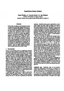
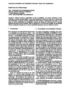
1@

2@

@ 14

@ 15

16@

@ 17

21 attributes: 1 – dam correct? 2 – sire correct? 3 – stated dam ph.gr. 1 4 – stated dam ph.gr. 2 5 – stated sire ph.gr. 1 6 – stated sire ph.gr. 2 7 – true dam ph.gr. 1 8 – true dam ph.gr. 2 9 – true sire ph.gr. 1 10 – true sire ph.gr. 2

A 18

A 19

20A

A 21

The grey nodes correspond to observable attributes.

3A

4A

5A

6A

7@

8@

9@

@ 10

11@

12@ 13@

11 12 13 14 15 16 17 18 19 20 21

– – – – – – – – – – –

offspring ph.gr. 1 offspring ph.gr. 2 offspring genotype factor 40 factor 41 factor 42 factor 43 lysis 40 lysis 41 lysis 42 lysis 43

Figure 1: Conditional independence graph of a graphical model for genotype determination and parentage verification of Danish Jersey cattle in the F-blood group system. another clique. In this case each distribution function represents the uncertainty about the values of the projections of ω0 onto the subspace corresponding to the maximal clique (i.e., the Cartesian product of the domains of the attributes contained in the maximal clique). As an example we consider an application of a graphical model for blood group determination of Danish Jersey cattle in the F-blood group system, whose primary purpose is parentage verification for pedigree registration [37]. The underlying domain is described by 21 attributes, eight of which are observable. The size of the domains of these attributes ranges from two to eight possible values. The total frame of discernment has 26 · 310 · 6 · 84 = 92 876 046 336 possible states. Therefore a decomposition of the expert knowledge about this domain is clearly necessary to make reasoning feasible. Figure 1 lists the attributes and shows the conditional independence graph of this graphical model, which was designed by human domain experts (the graphical model is a Bayesian network and thus the conditional independence graph is a directed acyclic graph). The grey nodes correspond to the observable attributes. The conditional independence graph reflects, as already said above, the conditional independences between the attributes of the underlying domain. In the case of a directed acyclic graph they can be read from the graph using a graph theoretic criterion called d-separation [35, 24]. What is to be understood by conditional independence depends on the uncertainty calculus the graphical model is based on. In the example at hand, which is a probabilistic graphical model, it means conditional stochastic independence of the random variables that are represented by the nodes of the graph. The joint probability distribution of these random variables is supposed to satisfy all independence relations represented by the conditional independence graph. Therefore, the joint probability distribution can be decomposed into a product of conditional


4

sire phenogroup 1 stated sire phenogroup 1 correct true sire F1 V1 V2 yes yes yes no no no

F1 V1 V2 F1 V1 V2

1 0 0 0.58 0.58 0.58

0 1 0 0.10 0.10 0.10

0 0 1 0.32 0.32 0.32

Table 1: Conditional probability distributions for a subgraph of the conditional independence graph shown in figure 1.

probability distributions (this is also called factorization). This product can easily be read from the conditional independence graph: There is exactly one factor for each attribute, which refers to the conditional probability distribution of the values of this attributes given an instantiation of the parents of this attribute [35, 54]. In the Danish Jersey cattle example, a decomposition of the joint probability distribution according to the conditional independence graph shown in figure 1 leads to a considerable simplification. Instead of having to determine the probability of each of the 92 876 046 336 elements of the 21-dimensional frame of discernment Ω, only 306 conditional probabilities in subspaces of at most three dimensions need to be specified. An example of a conditional probability table is shown in table 1, which is for the phenogroup 1 of the stated sire of a given calf conditioned on the phenogroup of the true sire of the calf and whether the sire was correctly identified. The numbers in this table are derived from statistical data and the experience of domain experts. The family of all 21 conditional probability tables forms the quantitative part of the graphical model for the Danish Jersey cattle example.

3

Evidence Propagation

After a graphical model has been constructed, it can be used to do reasoning. In the Danish Jersey cattle example, for instance, the phenogroups of the stated dam and the stated sire can be determined and the lysis values of the calf can be measured. From this information the probable genotype of the calf can be inferred and it is thus possible to assess whether the stated parents of the calf are the true parents. However, reasoning in a graphical model is not always completely straightforward. Considerations of efficiency make it often advisable to transform a graphical model into a form that is better suited for propagating the evidential knowledge and computing the resulting marginal distributions for the unobserved attributes. We briefly sketch here a popular efficient reasoning method known as clique tree propagation (CTP) [33, 8], which involves transforming the conditional independence graph into a clique tree. This transformation is carried out as follows: If the conditional independence graph is a directed acyclic graph, it is first turned into an undirected graph by constructing its associated moral graph [33]. A moral graph is constructed from a directed acyclic


5

1@$%() 3A

2@$%() 4A

7*%@

5A

8$@

1 C 4 8

6A

9*%@

#+@ 11

3 C 1 7

10$@ 12"@

2 C 6 10

8

2C./ 9 10

7 -C 8 11

9 -C 10 12

7

1C./

5 C 2 9

11 C012345 12 13

@!$% 13 @ 14

@ 15

16@

@ 17

A 18

A 19

20A

A 21

13 B 14

13 B 15

13B 16

13 B 17

14 B, 18

15 B, 19

16B, 20

17 B, 21

Figure 2: Triangulated moral graph (left) and clique tree (right) for the graphical model shown in Figure 1. The dotted lines are the edges added when parents were “married”. graph by “marrying” the parent nodes of all nodes (hence the name “moral graph”). This is done by simply adding undirected edges between the parents. The directions of all other edges are discarded. In general the moral graph satisfies a only subset of the independence relations of the underlying directed acyclic graph, so that this transformation may result in a loss of independence information. The moral graph for the Danish Jersey Cattle example is shown on the left in figure 2. The edges that were added when parents were “married” are indicated by dotted lines. In a second step, the undirected graph is triangulated. (If the conditional independence graph is an undirected graph right from the start, this is the first step to be carried out.) An undirected graph is called triangulated, if all cycles containing at least four nodes have a chord, where a chord is an edge that connects two non-adjacent nodes of the cycle. To achieve triangulation, it may be necessary to add edges, which may result in a (further) loss of independence information. In the Danish Jersey cattle example, however, the moral graph shown on the left in figure 2 is triangulated right away, so no new edges need to be introduced. Finally, the triangulated graph is turned into a clique tree by finding the maximal cliques, where a clique (see above) is a fully connected subgraph, and it is maximal, if it is not contained in another clique. In the clique tree there is one node for each maximal clique of the triangulated graph and its edges connect nodes that represent cliques having attributes in common. It should be noted that in general the clique tree is not unique, because often different sets of edges can be chosen. The clique tree for the Danish Jersey cattle example is shown on the right in figure 2. Detailed information on triangulation, clique tree construction and other related graph-theoretical problems can be found in [8].


6

The quantitative part of a graphical model, of course, has to be transformed, too. From the quantitative information of the original graphical model one has to compute a marginal distribution for each of the subspaces represented by the nodes of the clique tree. For the Danish Jersey cattle example, we have to compute a marginal distribution for the subspace formed by the attributes 1, 3, 7, one for the subspace formed by the attributes 1, 4, 8, and so on. That an appropriate factorization of the probability distribution can be found is ensured by the Hammersley-Clifford theorem [29]. It establishes a correspondence between the Markov properties (local, pairwise and global) of a strictly positive probability distribution P on Ω that are represented by a conditional independence graph and the factorization of P into a product of functions that depend only on the variables in the maximal cliques of the conditional independence graph. Having constructed a clique tree, which is merely a preliminary operation to make evidence propagation more efficient, we can finally turn to evidence propagation itself. Evidence propagation in clique trees is basically an iterative extension and projection process. When evidence about the value of an attribute becomes available, it is first extended to a clique tree node the attribute is contained in. This is done by conditioning the associated marginal distribution. We call this an extension, since by this conditioning process we go from restrictions on the values of a single attribute to restrictions on tuples of attribute values. Hence the information is extended from a single attribute to a subspace formed by several attributes. Then the conditioned distribution is projected to all intersections of the clique tree node with other nodes. Via these projections the information can be transferred to other nodes, where the process repeats: First it is extended to the subspace represented by the node, then it is projected to the intersections connecting it to other nodes. The process stops when all nodes have been updated. The propagation scheme outlined above and the subsequent computation of posterior marginal distributions for the unobserved attributes can easily be implemented by locally communicating node- and edge-processors. These processor also serve the task to let pieces of information “pass” each other without interaction. Such bypassing is necessary, if the propagation operations in the underlying uncertainty calculus are not idempotent, that is, if incorporating the same information twice can invalidate the results. This is the case, for example, in probabilistic reasoning. This problem is also the reason why the clique graph is usually required to be a tree: If there were loops, information could travel on two or more different paths to the same destination and thus be incorporated twice. Some other calculi, for instance, possibility theory, do not suffer from this inconvenience, so that the node- and edge-processor can be made simpler and loops do no harm (although they can make reasoning less efficient). A well-known interactive software tool for probabilistic reasoning in clique trees is HUGIN [1]. A similar approach was implemented in POSSINFER [22] for the possibilistic setting. That the propagation is efficient is obvious: If all available evidence is entered at the same time, distributing the information in the network requires only


7

two traversals of the clique tree. Of course, clique tree propagation is not the only possible propagation scheme. Others include bucket elimination [11, 57] and iterative proportional fitting [54]. Commonly used propagation algorithms differ from each other w.r.t. the network structures they support, but in most cases they are applicable independent of the given uncertainty calculus, provided, of course, the elementary operations like extension (conditioning) and projection have been adapted to this calculus [33, 35, 44]. A fairly general approach to reasoning under uncertainty in so-called valuation-based networks has been proposed in [46, 48, 47]. It can be applied, for example, to upper and lower probabilities [52], Dempster-Shafer theory of evidence [12, 13, 42, 43, 49], and possibility theory [56, 15, 16], and has been implemented in the software tool PULCINELLA [41].

4

Possibilistic Networks

Our review of graphical models in the preceding sections was strongly oriented at the well-known theory of probabilistic networks. In this section we turn to possibilistic networks, which are a much younger but very promising type of graphical models that can deal with uncertainty and imprecision. Their theory can be developed in close analogy to the probabilistic case. Technically, a possibilistic network is a graphical model whose quantitative component is a family of possibility distributions. Hence we start our discussion by briefly recalling possibility theory and its interpretations. Axiomatically, a possibility distribution π is a mapping from a reference set Ω to the unit interval. In contrast to a probability distribution, which is also defined to be such a mapping, a possibility distribution need not be normalized to one. That is, the sum (or the integral) of the degrees of possibility assigned by π to the elements of Ω need not be one. In the context of graphical models, we use a possibility distribution to specify imperfectly the current state ω0 of the domain under consideration. From an intuitive point of view, π(ω) quantifies the possibility that the proposition ω = ω0 is true: π(ω) = 0 means that ω = ω0 is impossible, whereas π(ω) = 1 means that it is possible without restriction. Any intermediary possibility degree π(ω) ∈ (0, 1) indicates that ω = ω0 is possible only with restrictions. That is, there is evidence supporting this proposition as well as evidence contradicting it. Of course, the above intuitive description is much too vague to fix a particular interpretation of degrees of possibility. Thus, similar to the probabilistic case where logical, empirical, and subjective interpretations of probability can be distinguished, there is a large variety of suggestions for semantics of a degree of possibility. Among them are the view of possibility distributions as epistemic interpretations of fuzzy sets [56], the axiomatic approach to possibility theory based on possibility measures [15, 16], and the approach that bases possibility theory on likelihoods [14]. In connection to Dempster-Shafer theory, possibility distributions are seen as contour functions of consonant belief functions [42], and in the framework of set-valued statistics, they are interpreted as falling shadows [53]. Furthermore, there are interpretations of possibility


8

theory that owe nothing to probability theory. We mention here the interpretation of possibility as similarity, which is related to metric spaces [39, 38, 40], and possibility as preference, which is justified mathematically by comparable possibility relations [17]. If one introduces possibility distributions as information-compressed representations of databases of (possibly imprecise) sample cases, as we will do in the next section, it is convenient to interpret them as (non-normalized) one-point coverages of random sets [34, 27]. This interpretation leads to very promising semantics [19, 20]. For instance, with this approach it is quite simple to establish Zadeh’s extension principle [55] as the appropriate way of extending operations on sets to operations on possibility distributions. It turns out that the extension principle is the only way of operating on possibility distributions that is consistent with this semantic background [18]. More precisely, let Ω be the set of all possible states of the world, ω0 ∈ Ω the current (but unknown) state of the world, (C, 2C , P ), C = {c1 , . . . , ck }, a finite probability space, and γ : C → 2Ω a set-valued mapping. C is seen as a set of contexts that have to be distinguished for a imprecise (set-valued) specification of ω0 . The contexts are supposed to describe different physical and observation-related frame conditions. P ({c}) is the (subjective) probability of the (occurrence or selection of the) context c. A set γ(c) is assumed to be the most specific correct set-valued specification of ω0 , which is implied by the frame conditions that characterize the context c. By “most specific set-valued specification” we mean that ω0 ∈ γ(c) is guaranteed to be true for γ(c), but is not guaranteed for any proper subset of γ(c). The resulting random set Γ = (γ, P ) is an imperfect (i.e. imprecise and uncertain) specification of ω0 . Let πΓ denote the one-point coverage of Γ (the possibility distribution induced by Γ), which is defined as πΓ : Ω → [0, 1], πΓ (ω) 7→ P ({c ∈ C | ω ∈ γ(c)}) . In a complete modeling, the contexts in C must be specified in detail, so that the relationships between all contexts cj and their corresponding specifications γ(cj ) are made explicit. But if the contexts are unknown or ignored, then πΓ (ω) is the total mass of all contexts c that provide a specification γ(c) in which ω0 is contained, and this quantifies the possibility of truth of the statement “ω = ω0 ” [19, 21]. As emphasized above, graphical models take advantage of conditional independence relations in order to reduce reasoning to operations on distributions on low-dimensional subspaces. Therefore a theoretical investigation of possibilistic graphical models has to start with the definition of an appropriate concept of conditional possibilistic independence. Such a definition allows us to introduce conditional independence graphs and to search for appropriate decomposition and factorization techniques. However, in contrast to the notion of probabilistic conditional independence, which has been well-known for a long time, there is still some discussion going on about an analogous concept for the possibilistic setting. The main reason for this is the fact that with possibility theory one can model two different kinds of imperfect knowledge: uncertainty and imprecision. Hence there are at least two alternative ways of approaching the task to define conditional possibilistic independence. In addition, different semantics for


9

possibility distributions may call for different concepts of conditional independence. For an overview, see [7]. Nevertheless, all suggestions for a concept of possibilistic conditional independence agree to the following general description: Let X, Y , and Z be three disjoint sets of attributes, X and Y non-empty. X is called independent of Y given Z w.r.t. a possibility distribution π on Ω, if for all instantiations of the attributes in Z, no information about the values of the attributes in Y changes the possibility degrees of the tuples over attributes in X. In other words: If the Z-values of ω0 are known, but arbitrary, then from additional information about the Y -values of ω0 no restrictions on the X-values of ω0 can be derived. In terms of projecting and conditioning possibility distributions we can rephrase this concept as follows: Suppose that a possibility distribution π is used to specify imperfectly the state ω0 . If crisp knowledge about the Z-values of ω0 is given, this distribution is conditioned w.r.t. the instantiations of the attributes in Z. If X and Y are independent given Z, then projecting the resulting conditional possibility distribution π directly to the attributes in X leads to the same distribution as first conditioning it first w.r.t. an arbitrary instantiation of the attributes in Y and only afterwards projecting it to the attributes in X. How conditioning and projection have to be defined depends on the chosen semantics of possibility distributions: If we view possibility theory as a special case of Dempster-Shafer theory by interpreting a possibility distribution as a representation of a consonant belief function or of a nested random set, then the concept of conditional independence can be derived from so-called Dempster conditioning [42]. If we see possibility distributions as (non-normalized) one-point coverages of random sets, we have to choose the conditioning and the projection operation in conformity with the extension principle. The resulting concept of conditional independence is conditional possibilistic non-interactivity [28]. For details, see [7]. It should be pointed out that both types of conditional independence mentioned above satisfy the semi-graphoid axioms which have been established as basic requirements for any reasonable concept of conditional independence in graphical models [35]. Possibilistic conditional independence derived from Dempster conditioning even satisfies the graphoid axioms [36], just as probabilistic conditional independence does. If we confine ourselves to conditional possibilistic non-interactivity in accordance with the interpretation of possibility distributions we preferred above, it is straightforward to define conditional possibilistic independence graphs: An undirected graph is called a conditional independence graph of a possibility distribution π, if for any three disjoint sets X, Y , and Z of nodes, X and Y non-empty, X is independent of Y given Z, if X and Y are separated by Z, i.e., if all paths from a node in X to a node in Y contain a node in Z. This definition assumes that the so-called global Markov property holds for π [54]. In contrast to probability distributions, where the equivalence of the global, local, and pairwise Markov property can be proven, in the possibilistic setting we have to rely on the global Markov property as the strongest of the three [18]. A proof of a possibilistic counterpart of the Hammersley-Clifford theorem [29] (see


10

lysis 40 lysis 41 lysis 42 lysis 43 genotype offspring {0, 1, 2} 6 0 6 V 2/V 2 0 5 4 5 {V 1/V 2, V 2/V 2} 2 6 0 6 * 5 5 0 0 F 1/F 1 Table 2: A small database with four sample cases

above) is given in [18]: A possibility distribution π on Ω has a decomposition into complete irreducible components, if it is decomposed w.r.t. a triangulated conditional independence graph G of π. The factorization of π w.r.t. this decomposition uses the minimum instead of the product, which is used in the probabilistic case, and the maximum instead of the sum. That is, π can be represented as the minimum of its maximum projections to the maximal cliques of G. It follows that evidence is propagated in possibilistic networks with a minimum/maximum scheme instead of the product/sum scheme of the probabilistic case.

5

Learning Possibilistic Networks from Data

A graphical model is a powerful tool to do reasoning—as soon as it is constructed. Its construction by human experts, however, can be tedious and time consuming. Therefore recent research in probabilistic as well as in possibilistic graphical models focused on learning them from a database of sample cases. In accordance with the two components of graphical models, one distinguishes between quantitative network induction, which serves to estimate the distribution functions of the factorization represented by a graphical model, and qualitative or structural network induction, which serves to find a conditional independence graph that captures (most) of the independences of the distribution function that is induced by the database. In possibilistic learning a special concern is to exploit the information contained in imprecise, i.e., set-valued, sample cases, which pose problems for probabilistic approaches. We start our discussion by showing how a database of imprecise sample cases induces a possibility distribution in the interpretation outlined in the preceding section. To this end we reconsider the Danish Jersey cattle example by looking at a small section of a database for this example as shown in figure 2. For simplicity, this database is reduced to five attributes. Each tuple describes one sample case, i.e., one calf. The first three tuples are imprecise, the fourth tuple is precise. The first tuple, for instance, represents the three precise tuples (0, 6, 0, 6, V 2/V 2), (1, 6, 0, 6, V 2/V 2), and (2, 6, 0, 6, V 2/V 2). This means that three states have to be regarded as possible alternatives. Analogously, the second tuple represents two alternatives which result from the imprecision in the attribute genotype offspring. The third tuple is imprecise, because it contains an unknown value, indicated by a star ‘*’, which can be interpreted


11

as representing the whole domain of the corresponding attribute. To induce a possibility distribution from this database, we interpret each tuple as corresponding to one context (see the preceding section). Assuming that the four sample cases are equally representative, it is reasonable to fix their probability of occurrence to 1/4. Note, however, that this is not enough for the probabilistic case, since it does not allow us to assign probabilities to the elementary events, i.e., the precise tuples in the domain underlying table 2. In the probabilistic setting, we may apply the insufficient reason principle, which states that alternatives in set-valued sample cases are equally likely, if no preferences are known. Assuming uniform distributions on set-valued sample cases leads to a refined database of 3 + 2 + 6 + 1 = 12 precise tuples, in which, for instance, (2, 6, 0, 6, V 2/V 2) has a probability of 1/3 ∗ 1/4 + 0 + 1/6 ∗ 1/4 + 0 = 3/24. This approach, however, unjustifiably introduces information about the relative probability of the possible values. In a possibilistic interpretation of the database, we obtain for the same tuple a degree of possibility of 1/4 + 0 + 1/4 + 0 = 1/2, since this tuple is considered to be possible in the first and in the third sample, but it is excluded in the other two. That is, no information is introduced that is not contained in the database. If we compute the possibility degrees for all tuples of the joint domain of the five attributes used in table 2, we arrive at an information-compressed interpretation of the database in the form of a possibility distribution. Quantitative Network Induction. Whereas quantitative network induction for both probabilistic and possibilistic networks is a rather trivial task, if all sample cases are precise (standard statistical techniques can be used in this case, see [50] for an overview), sample cases with missing values and especially with imprecise (set-valued) information pose a problem. This is true even for a possibilistic approach, which is better suited to handle set-valued information, since the imprecise tuples can “overlap”, thus preventing us from using simple techniques to compute maximum projections directly from the database. Fortunately, however, the database to learn from can be transformed by computing its closure under tuple intersection. From the transformed database all projections can be computed as efficiently as in the probabilistic case [5]. Qualitative Network Induction. The task to find a decomposition of the possibility distribution induced by a database of sample cases that best approximates this distribution w.r.t. a chosen class of conditional independence graphs is NP-hard for non-trivial classes of graphical models. This is true even if we confine ourselves to n-ary relations, which can be regarded as special cases of n-dimensional possibility distributions. For this reason, in analogy to learning probabilistic graphical models [9, 10, 51, 26], heuristics are unavoidable. These heuristics usually take the form of a search method and an evaluation measure. The evaluation measure estimates the quality of a given decomposition (a given conditional independence graph) and the search method determines which decompositions (which conditional independence graphs) are inspected. Often the search is guided by the value of the evaluation measure, since it is usually the goal to maximize (or to minimize) its value. [22] develops a rigid foundation of a learning algorithm for possibilistic networks.


12

It starts from a comparison of the nonspecificity of a given multivariate possibility distribution to the distribution represented by a possibilistic network, thus measuring the loss of specificity, if the multivariate possibility distribution is represented by the network. The measure of nonspecificity can be derived from Hartley information [25], in contrast to some evaluation measures for learning probabilistic networks, which are based on Shannon information [45]. In order to arrive at an efficient algorithm, an approximation for this loss of specificity is derived, which can be computed locally on the maximal cliques of the network. As the search method a generalization of the optimum weight spanning tree algorithm is used. Several other heuristic local evaluation measures for learning possibilistic networks, which can be used with different search methods, are discussed in [3, 4]. Implementations based on these theoretical results have successfully been applied to the Danish Jersey cattle example. For details, see [18, 4].

6

Conclusions

In this paper we reviewed the state of the art of possibilistic graphical models w.r.t. evidence propagation and learning and indicated similarities and differences to probabilistic graphical models. To summarize, probabilistic approaches serve for the exact modeling of uncertain, but precise data, since imprecise data cannot be represented by a single probability distribution. Possibilistic approaches serve for the approximate (information-compressed) modeling of uncertain and/or imprecise data. Therefore, probabilistic and possibilistic graphical models are useful in quite different domains of knowledge representation, which makes them cooperative rather than competitive. A topic of future work is to study in which way probabilistic and possibilistic data, obtained from expert knowledge and/or databases of sample cases, can be combined and then be represented as the quantitative part of a unified type of graphical model.

7

Acknowledgments

The concepts and methods of possibilistic graphical modeling presented in this paper were applied within the CEC-ESPRIT III BRA 6156 DRUMS II project (Defeasible Reasoning and Uncertainty Management Systems) and in a cooperation with Deutsche Aerospace for the design of a data fusion tool [2]. Furthermore, the learning algorithms have been implemented during the design of a data mining tool that is developed in the research center of DaimlerChrysler in Ulm, Germany.

References [1] S.K. Andersen, K.G. Olesen, F.V. Jensen, and F. Jensen. HUGIN — A Shell for Building Bayesian Belief Universes for Expert Systems. Proc. 11th Int. J.


13

[2]

[3]

[4]

[5]

[6] [7]

[8] [9]

[10]

[11]

[12] [13] [14] [15] [16]

Conf. on Artificial Intelligence (IJCAI’89, Detroit, MI, USA), 1080–1085. Morgan Kaufman, San Mateo, CA, USA 1989 J. Beckmann, J. Gebhardt, and R. Kruse. Possibilistic Inference and Data Fusion. Proc. 2nd European Congress on Fuzzy and Intelligent Technologies (EUFIT’94, Aachen, Germany), 46–47. Verlag Mainz, Aachen, Germany 1994 C. Borgelt and R. Kruse. Evaluation Measures for Learning Probabilistic and Possibilistic Networks. Proc. 6th IEEE Int. Conf. on Fuzzy Systems (FUZZ-IEEE’97, Barcelona, Spain), Vol. 2:1034–1038. IEEE Press, Piscataway, NJ, USA 1997 C. Borgelt and R. Kruse. Some Experimental Results on Learning Probabilistic and Possibilistic Networks with Different Evaluation Measures. Proc. 1st Int. J. Conf. on Qualitative and Quantitative Practical Reasoning (ECSQARU/FAPR’97, Bad Honnef, Germany), 71–85. Springer, Berlin, Germany 1997 C. Borgelt and R. Kruse. Efficient Maximum Projection of Database-Induced Multivariate Possibility Distributions. Proc. 7th IEEE Int. Conf. on Fuzzy Systems (FUZZ-IEEE’98, Anchorage, Alaska, USA), IEEE Press, Piscataway, NJ, USA 1997 W. Buntine. Operations for Learning Graphical Models. J. of Artificial Intelligence Research 2:159–224, 1994 L.M. de Campos, J. Gebhardt, and R. Kruse. Axiomatic Treatment of Possibilistic Independence. In: C. Froidevaux and J. Kohlas, eds. Symbolic and Quantitative Approaches to Reasoning and Uncertainty (LNCS 946), 77–88. Springer, Berlin, Germany 1995 E. Castillo, J.M. Gutierrez, and A.S. Hadi. Expert Systems and Probabilistic Network Models. Springer, New York, NY, USA 1997 C.K. Chow and C.N. Liu. Approximating Discrete Probability Distributions with Dependence Trees. IEEE Trans. on Information Theory 14(3):462–467. IEEE Press, Piscataway, NJ, USA 1968 G.F. Cooper and E. Herskovits. A Bayesian Method for the Induction of Probabilistic Networks from Data. Machine Learning 9:309–347. Kluwer, Dordrecht, Netherlands 1992 R. Dechter. Bucket Elimination: A Unifying Framework for Probabilistic Inference. Proc. 12th Conf. on Uncertainty in Artificial Intelligence (UAI’96, Portland, OR, USA), 211–219. Morgan Kaufman, San Mateo, CA, USA 1996 A.P. Dempster. Upper and Lower Probabilities Induced by a Multivalued Mapping. Ann. Math. Stat. 38:325–339, 1967 A.P. Dempster. Upper and Lower Probabilities Generated by a Random Closed Interval. Ann. Math. Stat. 39:957–966, 1968 D. Dubois, S. Moral, and H. Prade. A Semantics for Possibility Theory based on Likelihoods. Annual report, CEC–ESPRIT III BRA 6156 DRUMS II, 1993 D. Dubois and H. Prade. Possibility Theory. Plenum Press, New York, NY, USA 1988 D. Dubois and H. Prade. Fuzzy Sets in Approximate Reasoning, Part 1: Inference


14

[17] [18] [19]

[20]

[21]

[22]

[23] [24] [25] [26]

[27]

[28] [29] [30]

[31]

with Possibility Distributions. Fuzzy Sets and Systems 40:143–202. North Holland, Amsterdam, Netherlands 1991 D. Dubois, H. Prade, and R.R. Yager, eds. Readings in Fuzzy Sets for Intelligent Systems. Morgan Kaufman, San Mateo, CA, USA 1993 J. Gebhardt. Learning from Data: Possibilistic Graphical Models. Habilitation Thesis, University of Braunschweig, Germany 1997 J. Gebhardt and R. Kruse. A New Approach to Semantic Aspects of Possibilistic Reasoning. In: M. Clarke, S. Moral, and R. Kruse, eds. Symbolic and Quantitative Approaches to Reasoning and Uncertainty (LNCS 747), 151–159. Springer, Berlin, Germany 1993 J. Gebhardt and R. Kruse. On an Information Compression View of Possibility Theory. Proc. 3rd IEEE Int. Conf. on Fuzzy Systems (FUZZ-IEEE’94, Orlando, FL, USA), 1285–1288. IEEE Press, Picataway, NJ, USA 1994 J. Gebhardt and R. Kruse. POSSINFER — A Software Tool for Possibilistic Inference. In: D. Dubois, H. Prade, and R. Yager, eds. Fuzzy Set Methods in Information Engineering: A Guided Tour of Applications, 407–418. J. Wiley & Sons, New York, NY, USA 1996 J. Gebhardt and R. Kruse. Tightest Hypertree Decompositions of Multivariate Possibility Distributions. Proc. Int. Conf. on Information Processing and Management of Uncertainty in Knowledge–Based Systems (IPMU’96), 923–927. Granada, Spain 1996 J. Gebhardt and R. Kruse. Automated Construction of Possibilistic Networks from Data. J. of Applied Mathematics and Computer Science, 6(3):101–136, 1996 D. Geiger, T.S. Verma, and J. Pearl. Identifying Independence in Bayesian Networks. Networks 20:507–534. J. Wiley & Sons, Chichester, England, 1990 R.V.L. Hartley. Transmission of Information. The Bell Systems Technical Journal 7:535–563, 1928 D. Heckerman, D. Geiger, and D.M. Chickering. Learning Bayesian Networks: The Combination of Knowledge and Statistical Data. Machine Learning 20:197–243, Kluwer, Dordrecht, Netherlands, 1995 K. Hestir, H.T. Nguyen, and G.S. Rogers. A Random Set Formalism for Evidential Reasoning. In: I.R. Goodman, M.M. Gupta, H.T. Nguyen, and G.S. Rogers, eds. Conditional Logic in Expert Systems, 209–344. North-Holland, Amsterdam, Netherlands 1991 E. Hisdal. Conditional Possibilities, Independence, and Noninteraction. Fuzzy Sets and Systems 1:283–297. North Holland, Amsterdam, Netherlands 1978 V. Isham. An Introduction to Spatial Point Processes and Markov Random Fields. Int. Statistics Review 49:21–43, 1981 F. Klawonn, J. Gebhardt, and R. Kruse. Fuzzy Control on the Basis of Equality Relations with an Example from Idle Speed Control. IEEE Transactions on Fuzzy Systems 3:336–350. IEEE Press, Piscataway, NJ, USA 1995 R. Kruse, J. Gebhardt, and F. Klawonn. Foundations of Fuzzy Systems. J. Wiley


15

& Sons, Chichester, England 1994 [32] R. Kruse, E. Schwecke, and J. Heinsohn. Uncertainty and Vagueness in Knowledge Based Systems: Numerical Methods. Springer, Berlin, Germany 1991 [33] S.L. Lauritzen and D.J. Spiegelhalter. Local Computations with Probabilities on Graphical Structures and Their Application to Expert Systems. Journal of the Royal Statistical Society, Series B 2(50):157–224. Blackwell, Oxford, United Kingdom 1988 [34] H.T. Nguyen. Using Random Sets. Information Science 34:265–274, 1984 [35] J. Pearl. Probabilistic Reasoning in Intelligent Systems: Networks of Plausible Inference (2nd edition). Morgan Kaufmann, San Mateo, CA, USA 1992 [36] J. Pearl and A. Paz. Graphoids — A Graph Based Logic for Reasoning about Relevance Relations. In: B.D. Boulay et al., eds. Advances in Artificial Intelligence 2, 357–363. North-Holland, Amsterdam, Netherlands 1991 [37] L.K. Rasmussen. Blood Group Determination of Danish Jersey Cattle in the Fblood Group System. Dina Research Report 8, Dina Foulum, Tjele, Denmark 1992 [38] E.H. Ruspini. The Semantics of Vague Knowledge. Rev. Internat. Systemique 3:387–420, 1989 [39] E.H. Ruspini. Similarity Based Models for Possibilistic Logics. Proc. 3rd Int. Conf. on Information Processing and Management of Uncertainty in Knowledge Based Systems (IPMU’96), 56–58. Granada, Spain 1990 [40] E.H. Ruspini. On the Semantics of Fuzzy Logic. Int. J. of Approximate Reasoning 5. North-Holland, Amsterdam, Netherlands 1991 [41] A. Saffiotti and E. Umkehrer. PULCINELLA: A General Tool for Propagating Uncertainty in Valuation Networks. Proc. 7th Conf. on Uncertainty in Artificial Intelligence (UAI’91, Los Angeles, CA, USA), 323–331. Morgan Kaufman, San Mateo, CA, USA 1991 [42] G. Shafer. A Mathematical Theory of Evidence. Princeton University Press, Princeton, NJ, USA 1976 [43] G. Shafer and J. Pearl. Readings in Uncertain Reasoning. Morgan Kaufman, San Mateo, CA, USA 1990 [44] G. Shafer and P.P. Shenoy. Local Computations in Hypertrees (Working Paper 201). School of Business, University of Kansas, Lawrence, KS, USA 1988 [45] C.E. Shannon. The Mathematical Theory of Communication. The Bell Systems Technical Journal 27:379–423. 1948 [46] P.P. Shenoy. A Valuation-based Language for Expert Systems. Int. J. of Approximate Reasoning 3:383–411. North-Holland, Amsterdam, Netherlands 1989 [47] P.P. Shenoy. Valuation Networks and Conditional Independence. Proc. 9th Conf. on Uncertainty in AI (UAI’93), 191–199. Morgan Kaufman, San Mateo, CA, USA 1993 [48] P.P. Shenoy and G.R. Shafer. Axioms for Probability and Belief-Function Propagation. In: R.D. Shachter, T.S. Levitt, L.N. Kanal, and J.F. Lemmer. Uncertainty


16

in Artificial Intelligence 4, 169–198. North Holland, Amsterdam, Netherlands 1990 [49] P. Smets and R. Kennes. The Transferable Belief Model. Artificial Intelligence 66:191–234. Elsevier, Amsterdam, Netherlands 1994 [50] D. Spiegelhalter, A. Dawid, S. Lauritzen, and R. Cowell. Bayesian Analysis in Expert Systems. Statistical Science 8(3):219–283, 1993 [51] T.S. Verma and J. Pearl. An Algorithm for Deciding if a Set of Observed Independencies has a Causal Explanation. Proc. 8th Conf. on Uncertainty in Artificial Intelligence (UAI’92, Stanford, CA, USA), 323–330. Morgan Kaufman, San Mateo, CA, USA 1992 [52] P. Walley. Statistical Reasoning with Imprecise Probabilities. Chapman & Hall, New York, NY, USA 1991 [53] P.Z. Wang. From the Fuzzy Statistics to the Falling Random Subsets. In: P.P. Wang, ed. Advances in Fuzzy Sets, Possibility and Applications, 81–96. Plenum Press, New York, NY, USA 1983 [54] J. Whittaker. Graphical Models in Applied Multivariate Statistics. J. Wiley & Sons, Chichester, England 1990 [55] L.A. Zadeh. The Concept of a Linguistic Variable and Its Application to Approximate Reasoning. Information Sciences 9:43–80, 1975 [56] L.A. Zadeh. Fuzzy Sets as a Basis for a Theory of Possibility. Fuzzy Sets and Systems 1:3–28. North-Holland, Amsterdam, Netherlands 1978 [57] N.L. Zhang and D. Poole. Exploiting Causal Independence in Bayesian Network Inference. Journal of Artificial Intelligence Research 5:301–328, 1996


17