Potential impact of sea surface temperature on rainfall over the ...

Dado and Takahashi Progress in Earth and Planetary Science (2017) 4:23 DOI 10.1186/s40645-017-0137-6

Progress in Earth and Planetary Science

RESEARCH ARTICLE

Open Access

Potential impact of sea surface temperature on rainfall over the western Philippines Julie Mae B. Dado1*

and Hiroshi G. Takahashi1,2

Abstract The study used a 5 km-resolution regional climate model, the Advanced Research Weather Research and Forecasting Model, to quantify the potential impact of sea surface temperature (SST) west of the Philippines on summer monsoon rainfall on the northwestern coast of the country. A set of control simulations (CTL) driven by ERA-Interim reanalysis data and the monthly National Oceanic and Atmospheric Administration Optimum Interpolation SST dataset was performed for the months of June to August of 1982–2012. A second set of simulations driven by climatological SST values was performed for the same period. The difference between these two simulation sets is analyzed to determine the sensitivity of rainfall to interannual variations in local SST, not remote SST, via a regional climate model. The CTL simulations represented spatial and temporal variations in rainfall well, yielding realistic climatological rainfall values with high spatial correlations with observations. The interannual correlation of monthly rainfall over the northwestern region of the Philippines was also high when compared to observations. The results showed that positive SST anomalies west of the Philippines induced positive rainfall anomalies in the northwestern Philippines via an increase in latent heat flux from the sea surface, implying that summer monsoon rainfall in the northwestern Philippines is modulated by interannual variations in SST west of the Philippines. The impact of SST on latent heat flux and rainfall were 20–40%, greatly exceeding the 7% approximation from the Clausius–Clapeyron equation, which can be explained by the enhancement of low-level winds and a weak warming of surface air temperature over the ocean. Keywords: Summer monsoon, Rainfall, Sea surface temperature, Regional climate model

Introduction The Philippines is located in an area primarily affected by the Asian summer monsoon. Specifically, the northwestern side of the country is affected by this system, which is known locally as the southwest monsoon (SWM). The SWM is part of the western North Pacific Monsoon within the Asian-Pacific summer monsoon system (Wang and LinHo 2002). The subsystems within the Asian summer monsoon are known to interact with each other. The monsoon onset of regions to the west of the Philippines, specifically Indochina Peninsula and South China Sea (SCS), is associated with the development in the circulation and convective features in the tropical East Indian Ocean (Ding and Chan 2005). The Asian monsoon is a complex system, but the past decade have seen significant advances in understanding climate * Correspondence: [email protected]; [email protected] 1 Department of Geography, Tokyo Metropolitan University, Minami-Osawa 1-1, Hachioji, Tokyo 192-0397, Japan Full list of author information is available at the end of the article

over the region through the Monsoon Asian HydroAtmosphere Scientific Research and Prediction Initiative (MAHASRI) project (Matsumoto et al. 2016). Rainfall is an important characteristic of the SWM season because these winds carry warm, moist air, which has a higher potential for convective activity. The northwestern regions of the Philippines experience a rainy season during June to September. A significant percentage (43%) of the mean annual rainfall in the Philippines is associated with the SWM season, which is essential for supplying water for agriculture, energy, and domestic use (Asuncion and Jose 1980; Cayanan et al. 2011). Although there has been a general decline in the SWM mean rainfall over northwestern Philippines (Cruz et al. 2013), intense rainfall episodes still occur during the SWM season, which can result in heavy flooding. The oceans surrounding the Philippines have a major impact on its regional climate. Large-scale oceanic impacts, including El Niño–Southern Oscillation (ENSO, Lyon and Camargo 2009; Villafuerte and

© The Author(s). 2017 Open Access This article is distributed under the terms of the Creative Commons Attribution 4.0 International License (http://creativecommons.org/licenses/by/4.0/), which permits unrestricted use, distribution, and reproduction in any medium, provided you give appropriate credit to the original author(s) and the source, provide a link to the Creative Commons license, and indicate if changes were made.

Dado and Takahashi Progress in Earth and Planetary Science (2017) 4:23

Matsumoto 2015), have been examined in many studies. However, the impact of local sea surface temperature (SST) on the country is not well understood. Thus, there is a need to examine the local SST impact on regional rainfall over the Philippines. Studies have noted the relationship between SST and atmosphere through the exchange of surface fluxes (Deser et al. 2010). The amount of near-surface moisture for convective rainfall is sensitive to SST through the Clausius–Clapeyron relationship and is strongly associated on interannual timescales over oceanic regions (Wentz and Schabel 2000). In general, higher SSTs correspond to increases in precipitation (Vecchi and Harrison 2002; Trenberth and Shea 2005). In addition, a recent study showed that precipitation tends to increase linearly with increasing SST over tropical monsoon basins, suggesting a noticeable impact of SST on tropical precipitation (Roxy 2014). In the western North Pacific (WNP) region, the correlation between local rainfall and SST in the boreal summer is negative indicating that atmospheric dynamics are more dominant than ocean conditions in determining the rainfall variability of this region (Trenberth and Shea 2005; Wang et al. 2005). This relationship may be explained by the monsoon activity during this season. The summer monsoon drives rainfall but it also leads to SST cooling, hence the negative correlation between local rainfall and SST. Moreover, Trenberth and Shea (2005) also showed the covariability between surface temperature and precipitation, and although relationship is negative in WNP, it would be interesting to isolate the SST effect alone. Note that impact of local SST on rainfall variation in this region has not been evaluated yet, although these previous studies have indicated that SST cannot be the main driver of rainfall in this region. However, it is difficult to quantify the impact of SST on rainfall from observational datasets because of strong air– sea interactions (Peralta and Narisma 2014). This is similar to a mid-latitude winter monsoon case over the Sea of Japan (Takahashi and Idenaga 2013; Takahashi et al. 2013), although the range in surface air temperature is quite different. Higher SSTs bring higher latent heat fluxes under the same atmospheric conditions due to higher water vapor pressures on the sea surface, which is explained by the Clausius–Clapeyron equation. At the same time, the evaporation over the sea surface decreases the SST. In SWM condition, the strong monsoon westerly also increases latent heat flux which brings abundant rainfall to the northwestern Philippines. And since rainfall on the northwestern Philippines is predominantly controlled by the SWM airflow, the SST effect is seemingly hidden in all these dynamics. These dynamics are highly coupled, and while it is difficult to isolate the one-way impacts from observational data alone,

Page 2 of 12

numerical experiments are useful for understanding and quantifying such one-way impacts. The SWM months also coincide with high tropical cyclone (TC) activity in the WNP basin including the Philippines (Cinco et al. 2016; Lyon and Camargo 2009; Takahashi and Yasunari 2006). This high frequency of TC makes a substantial contribution on rainfall over the monsoon trough (Takahashi et al. 2015a), especially in the northern island of Luzon (Cinco et al. 2016). It has also been shown that SWM rainfall is enhanced in the presence of TCs (Cayanan et al. 2011; Kubota and Wang 2009), and as such, this study also attempts to isolate the TC effect in the analysis of SWM rainfall. To determine the contribution of SST to rainfall in a statistically robust manner, long-term or multiple-case experiments are required, as the atmospheric response to SST anomalies can vary under different atmospheric conditions (Peng et al. 1997). Moreover, long-term climate simulations can be used to investigate the extent to which interannual variations in SST affect regional climate. In this study, we examined the response of rainfall associated with the SWM from SST forcing located west of the Philippines. We attempted to isolate the impact of SST alone, neglecting feedback from the atmosphere to the ocean, by applying SST as the boundary condition in a regional climate model. We focused on the effects of SST located west of the Philippines, as SWM winds pass through this area before arriving on the northwestern coast of the country. The SST–rainfall relationship is important in further understanding the hydroclimate within this region which translates in its significance in economic sectors such as agriculture. The methodology is discussed in detail in the “Methods/Experimental” section, and an evaluation of the performance of the model and quantification of the SST impact is described in the “Results” section. Changes in latent heating and the lack of a tropical cyclone (TC) effect are discussed in the “Discussion” section, and a summary is presented in the “Conclusions” section.

Methods/Experimental Model and experimental setup

We used a non-hydrostatic regional climate model, the Advanced Research Weather Research and Forecasting Model (WRF) ver. 3.6.1 with the Advanced Research WRF dynamical core (Skamarock et al. 2008) to examine the impact of SST on precipitation. The initial and lateral boundary conditions used were from the ERAInterim reanalysis data (Berrisford et al. 2009) of the European Centre for Medium-Range Weather Forecasts, and SST data were from the Optimum Interpolation Sea Surface Temperature (OISST) ver. 2 (Reynolds et al. 2002). A set of control simulations (CTL) was performed for the months of June to August for the years 1982–


2012. Temporally interpolated monthly values of SST were prescribed every 6 h. Multi-year simulations were performed to investigate the robustness of the atmospheric response to SST forcing under various atmospheric conditions. The simulation period was from May 27 to September 1 of each year. The first 5 days served as the simulation warm-up time and were not included in the analysis. The horizontal grid resolution of the first domain was 25 km, while that of the two-way nested domain was 5 km. Both domains had 33 terrain-following levels. Figure 1 shows the model domains. The cumulus convective parameterization (CCP) scheme was not applied to the two domains in this study because a series of test simulations with CCP yielded unrealistic amounts of rainfall. Previous studies have shown that WRF is able to capture rainfall in Asian monsoon regions without convective parameterization (Sugimoto and Takahashi 2017; Sugimoto and Takahashi 2016;

Page 3 of 12

Takahashi et al. 2010). Three schemes were used: the WRF single-moment six-class microphysics scheme (Hong and Lim 2006), the Mellor–Yamada–Janjić planetary boundary layer scheme (Janjić 1994), and the unified Noah land surface model (Tewari et al. 2004). High-resolution model can represent topography and land–sea contrast in detail; thus, analysis of the SST impact was carried out using the 5 kmmodel results. Sensitivity experiments

To analyze the effect of interannual variations in SST, we performed a set of sensitivity experiments. In this experiment, the 31-year mean monthly climatological SST was computed using OISST, and then applied to the same 31-year time period as the CTL simulations (hereinafter referred to as the CLM runs). The numerical designs of the CTL and CLM runs were the same, except for application of the SST. The

Fig. 1 Topographical map of the study area showing the domains used in the model. The gray shading indicates elevation in meters. Domain 1 (D01) and domain 2 (D02) have grid resolutions of 25 and 5 km, respectively. The red dashed box shows the reference region for sea surface temperature (WSST; 12–18° N, 115–120° E), and the blue dashed box shows the reference region for rainfall (WPH; 14–19° N, 119.5–121° E)


difference between the CTL and CLM runs represented the atmospheric response to the interannual SST variability. This experimental design was based on a previous study to detect local SST impact (Takahashi et al. 2015b). The local SST impact can be isolated using this design with the remote SST effect already included in the large-scale atmospheric conditions used as lateral boundary forcing for both the CTL and CLM experiments. Observational datasets used for the evaluation

The simulated rainfall from the CTL runs was evaluated using data from the Asian Precipitation Highly-Resolved Observational Data Integration Towards Evaluation (APHRODITE) of Water Resources (Yatagai et al. 2012) and the Global Precipitation Climatology Project (GPCP) ver. 2.2 (Adler et al. 2003), and the low-level circulations were compared with data from the Japanese 55-year Reanalysis (JRA55; Kobayashi et al. 2015), which differed from the driving atmospheric datasets used in the simulations. Figure 1 shows the regions selected for a targeted analysis of the effect of SST on the climate of the northwestern Philippines. The red dashed box shows the reference region for SST (hereinafter referred as

Page 4 of 12

WSST; 12–18° N, 115–120° E), and the blue dashed box shows the reference region for rainfall (hereinafter referred as the northwestern region of the Philippines (WPH); 14–19° N, 119.5–121° E). Tropical cyclone (TC) track data

The number of unique TCs crossing the first domain of the simulation (D01) in Fig. 1 is counted for the months of June–August of 1982–2012 based on the best track data from the Joint Typhoon Warning Center (JTWC). For each month, years with TC counts below the mean were considered as low-TC years, which we assumed to be more representative of the SWM climate. The SST impact under this low-TC condition is explained in detail in the “Discussion” section.

Results Evaluation of CTL simulations

First, we evaluated the performance of the simulated regional climate over the northwestern Philippines. The simulated 850 hPa horizontal winds in domain 2 were compared with JRA55, which differed from the ERA-Interim boundary forcing data. The low-level monsoon southwesterlies were

a

b

c

d

e

f

Fig. 2 Climatological monthly 850 hPa level winds (m s−1) from 1982 to 2012 over domain 2, calculated by the CTL simulation (d–f) and compared with the JRA55 (a–c). Monsoon strength, denoted by the zonal wind component, is shown as shaded contours in the figure


well simulated for the months of June, July, and August (Fig. 2). Furthermore, the model captured the monsoon strength, denoted by the zonal wind component. The spatial pattern of the simulated rainfall in the CTL experiment was evaluated by comparing the climatological monthly total for each month with the APHRODITE dataset (Fig. 3). APHRODITE has data for 1950–2007; however, we only considered the years 1982–2007 to remain consistent in reproducing climatological values for both simulations and observations. We verified that the results were nearly the same when using climatological rainfall values for 1982–2012. To facilitate the comparison between the observations and simulations, the simulated rainfall over the ocean was masked because the APHRODITE dataset was limited to the terrestrial region. The spatial distribution of climatological rainfall was represented well by the CTL. It was able to show the west–east gradient in rainfall in the assessed months. In addition, the spatial distribution of higher rainfall values in the northwestern portion was noted in both the observational and simulated data. However, peaks in rainfall differed slightly, and the model produced higher rainfall values, predominantly in areas with high elevations. This may represent a positive bias of the simulated rainfall over high-elevation

Page 5 of 12

regions. In addition, the APHRODITE data were mostly obtained from coastal observation stations which can result in its underestimation of rainfall in high-elevated regions. In addition, we validated the climatological simulated rainfall against the GPCP data, which were produced from different observations, and noted a spatial distribution similar to that for APHRODITE (not shown). The CTL monthly rainfall values in the northwestern Philippines (WPH in Fig. 1) were compared with APHRODITE monthly rainfall values for 1982–2007. Similarly, the GPCP monthly mean rainfall was obtained for the same WPH region for the years 1982–2012. Ocean grid points in the WPH region were included when comparing the CTL rainfall with the GPCP rainfall. The seasonal variation in the climatological monthly rainfall was simulated well by the model when compared with APHRODITE and GPCP data, and the WRF rainfall showed a similar seasonal peak in August (not shown). Furthermore, we analyzed the interannual rainfall variations in the region west of the Philippines (WPH in Fig. 1) for both the observational and simulated data as scatter plots of the observed and simulated monthly precipitation for the WPH region (Fig. 4). The comparison revealed a high correlation between the monthly total

a

b

c

d

e

f

Fig. 3 Climatological monthly terrestrial precipitation (mm month−1) from 1982 to 2007 over domain 2, calculated by the CTL simulation (d–f) and compared with the APHRODITE dataset (a–c)


a

b

Fig. 4 a Scatter plot of the monthly total rainfall (mm month−1) from the CTL simulations compared with APHRODITE data for 1982–2007. b Scatter plot of monthly mean of daily rainfall (mm day−1) from the CTL simulations compared with GPCP data for 1982–2012

rainfall from APHRODITE and the CTL simulation for the years 1982–2007 for the WPH region (Fig. 4a). The interannual seasonal mean (June to August) correlation coefficient was 0.69. In addition, the comparison revealed a high correlation between the monthly means of daily rainfall from the GPCP data and the CTL simulation (Fig. 4b) for the WPH region, with an interannual correlation of the seasonal mean of 0.80. These interannual correlations were statistically significant at a 99.9% confidence limit, determined using Student’s t test. These results indicate that the CTL runs captured the summer rainfall in the WPH region well. Despite differences in the amount of monthly rainfall, the WRF CTL runs were able to capture the interannual and seasonal variations in precipitation in the WPH region; for the purpose of this study, the model demonstrated acceptable performance.

Page 6 of 12

Sensitivity of rainfall to SST variability

To estimate the local impact of SST on rainfall spatially, we generated regression maps using Theil–Sen method to show the interannual variation in the sensitivity of monthly rainfall with area-averaged SST anomalies in the WSST region for the months of June, July, and August (Fig. 5). The sensitivity of rainfall to SST was defined as the difference between the CTL and CLM experiments. The regression coefficient was calculated using the sensitivity of the meteorological variables and the area-averaged SST anomalies. Because we used the same atmospheric boundary conditions for the CTL and CLM experiments, we could not extract the impact of remote SST. Therefore, we only evaluated the impact of SST within the model domain. The simulated results were transformed into coarser values at each 1-degree grid point from the original 5 km output to minimize noise. Similarly, the SST anomaly was defined as the difference between the CTL and CLM values averaged over the WSST region (Fig. 1). Positive rainfall sensitivity to 1 K SST warming was noted over the whole calculation domain (Fig. 5), which can be explained by the increase in latent heat flux due to the increase in SST. A detailed description of the process underlying rainfall sensitivity to changes in SST is given in the “Discussion” section. Higher and statistically significant sensitivity was observed for oceanic rainfall near the WSST region. Statistically significant values were noted in the WPH region, and August had the highest regression coefficient (Fig. 5). These maps show that monthly rainfall in the WPH increased by ~100 mm K−1 SST warming in the WSST. Because the interannual standard deviation of SST over the WSST was between 0.4 and 0.6 K, 40–60 mm of interannual variation in monthly rainfall could be attributed to the interannual variation of SST over the WSST (Fig. 5). Because the average climatological rainfall was ~500 mm per month in this region, the contribution of SST to interannual rainfall variation was not negligible. To understand the interannual relationship between SST and rainfall over and around the Philippines, we examined the time series of the SST anomaly over the WSST region and rainfall sensitivity (CTL − CLM) over the WPH region for June, July, and August (Fig. 6). A positive or negative SST anomaly generally corresponded to positive or negative rainfall sensitivity, respectively. This relationship is evident in the scatter plots (Fig. 6d–f), which clearly show that the sensitivity of rainfall in the WPH region increased with SST in the WSST region. Because the relationship is almost linear, the impact of SST on rainfall can be quantified on an interannual timescale. Using the Theil–Sen slope estimator method, the calculated regression coefficient of rainfall in the WPH region on the area-averaged SST over the WSST region increased


a

b

Page 7 of 12

c

Fig. 5 Spatial map of the regression coefficients (mm K−1) of the sensitivity of monthly rainfall to the monthly SST anomaly of the WSST reference region for 1982–2012 for the months of a June, b July, and c August. Significant values at the 90% significance level are marked with plus signs, as determined by the correlation coefficients based on 29 degrees of freedom. The rainfall anomalies were remapped to a 1° grid resolution

by 80.65, 78.86, and 99.69 mm K−1 SST warming in the WSST region for the months of June, July, and August, respectively. This accounted for 23–37% of the climatological monthly rainfall in the WPH region, depending on the month considered. These results indicate that it is important to account for the impact of SST on rainfall in the WPH region. The mechanism behind this relationship is discussed in the following section.

Discussion Quantification of the sensitivity of latent heat flux to SST

The major sources of water vapor for rainfall in the WPH region are the evaporation from the western

seas of the Philippines, which is windward of the Philippines in the summer, and water vapor transport due to the monsoon southwesterlies, especially during the SWM season. In our experiment, water vapor transport from the lateral boundary (see the western lateral boundary of Fig. 1) should have been the same, because the same lateral boundary conditions were used. Therefore, any changes in water vapor should be explained by changes in the evaporation, which is directly related to latent heat flux, within the calculation domains. Similarly, we regressed the interannual latent heat flux sensitivity to area-averaged SST anomaly in the WSST

a

b

c

d

e

f

Fig. 6 Time series (a–c) and scatter plots (d–f) of the area-averaged monthly mean SST anomalies in the WSST region and monthly precipitation difference (PCTL − PCLM) in the WPH region for June, July, and August, respectively. The dashed line in the scatter plot indicates the linear relationship between SST anomaly and rainfall sensitivity estimated using the Theil–Sen method


a

b

Page 8 of 12

c

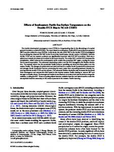
Fig. 7 Spatial map of the regression coefficients of the sensitivity of latent heat flux (lhf) to the monthly SST anomaly of the WSST reference region for 1982–2012 for the months of a June, b July, and c August. The values are shown in percentage relative to the 31 yr.-mean lhf from CTL

region for the months of June, July, and August. The values are expressed in percentage relative to the 31year mean latent heat from CTL experiment. The latent heat flux increased by 20–40% per 1 K SST warming in the WPH region, with larger increases in the seas west of the Philippines (Fig. 7). This increase in the latent heat flux was higher than the simulated change in rainfall in the WPH region. Because the relative humidity change at 2 m height was very small (within −2–2%) in most of the domain (Fig. 8), we can infer that the increase in water vapor due to the increase in latent heat was mostly converted into rainfall. To analyze this large increase in latent heat in the domain, the bulk formula for the latent heat flux from the sea into the atmosphere can be given as. lE = lρβCHU(qsat(Ts) − q), where l is the latent heat of vaporization, E is the amount of evaporation, ρ is the density of air, β is the efficiency of evaporation which is 1 over water, CH is a mixing constant,

a

b

U is the wind velocity, and Ts is the SST over the western seas of the Philippines. qsat is the saturated specific humidity at Ts, and q is the specific humidity of the lower atmosphere. Therefore, latent heating can be explained by wind velocity and the difference between the saturated specific humidity at SST and the surface specific humidity. Changes in wind speed and specific humidity are likely critical in explaining the much larger sensitivities in latent heat flux over the WSST regions than expected from the Clausius–Clapeyron equation. The changes in the wind speed per 1 K SST warming were mostly positive (within 10%), which increased the latent heat flux over the WSST region by 5–10% percent (Fig. 9). This increase in wind speed was associated with a downward transport of momentum due to the development of the planetary boundary layer height (e.g., Stull 2006) and enhancement of regional circulation that is accompanied by latent heating and convective activity. The 2 m air temperature increase was