Practical and Economic Aspects of the Ex-Situ ... - ACS Publications

Article pubs.acs.org/EF

Practical and Economic Aspects of the Ex-Situ Process: Implications for CO2 Sequestration Sohrab Zendehboudi,*,† Alireza Bahadori,‡ Ali Lohi,§ Ali Elkamel,† and Ioannis Chatzis† †

Department of Chemical Engineering, University of Waterloo, Waterloo, Ontario, Canada School of Environment, Science and Engineering, Southern Cross University, Lismore, NSW, Australia § Department of Chemical Engineering, Ryerson University, Toronto, Ontario, Canada ‡

S Supporting Information *

ABSTRACT: The risk of CO2 leakage and the very slow rate of CO2 dissolution in brine present major technical challenges for secure implementation of CO2 sequestration at large scale in saline aquifers. To tackle these issues, a new technology based on Ex-Situ Dissolution Approach (ESDA) was developed recently aiming at dissolving CO2 in brine phase prior to injection into the aquifer to eliminate or minimize the risk of leakage and accelerate CO2 dissolution rate in brine. The ESDA is based on the mass transfer from CO2 droplets into brine in cocurrent pipeline flow. This paper presents mass transfer modeling associated with the ESDA process concerning the evolution of the droplet size and the pressure change along the pipeline. In addition, a technical and economic feasibility of the ESDA in comparison with the standard carbon capture and storage (CCS) technologies is presented. Various aspects such as CO2 displacement, geochemical reactions, CO2 leakage, pressure build-up, well spacing, and dissolution efficiency for the ESDA are also discussed. This study enables the evaluation of the ESDA process for CO2 sequestration through a systematic way.

1. INTRODUCTION In the past few decades, carbon capture and storage (CCS) has been an attractive and a viable option to lower the CO2 concentration emitted into the atmosphere.1−4 The global potential for storing CO2 in deep saline formations was estimated between 400 and 10000 Gt of CO2 by the International Energy Agency Greenhouse Gas (IEAGHG) research and development program in early 1990s.1−4 Thus, CCS in deep aquifers (e.g., saline aquifers) is considered as one of the promising techniques to mitigate this issue and to lessen the growing effects of the global warming.1,2,4−7 Technically, it is now feasible to inject large amounts of CO2 in deep sedimentary basins and store it for a long time at a reasonable cost, if acceptable from the perspective of long-term environmental impacts.4,5 Over the years, scientists proposed several different methods (e.g., direct injection, mineral carbonization) to sequester CO2 into the oceans and deep formations.4,5,8 However, the process modeling and feasibility assessment of each technology has been complicated because of a lack of thorough understanding of the complex transport phenomena during the disposal process.5,8−10 Moreover, safety issues related to CO2 leakage present challenges to researches and more technical attention is required to tackle this uncertain area by nature.5,9,11,12 A number of sequestration scenarios proposed to date focused mainly on direct injection of CO2 in the form of supercritical or liquid state using injection wells at depths of 2000 m below surface or greater. Two main problems for such methodologies are that it is not easy to make sure the brine phase efficiently dissolves the injected CO2 and also that the onset time for convection regime is fairly long.5,9,11 Technologies currently available for the CO2 storage in saline aquifers face some technical challenges and issues.8,9,11,13 In the current practice for CCS technology, it is assumed that CO2 is injected as a free single phase into the target formation. This © 2012 American Chemical Society

phase is typically 10−40% less dense than the resident brine. Hence, driven by density contrasts, CO2 flows upward by buoyancy forces, collecting at the top of the formation, and it can leak through fractures or through abandoned wells to the surface. CO2 leaking out of the subsurface is the most important potential problem due to the fact that the buoyancy-driven movement of CO2 can lead to a decrease in the amount of the immobilized CO2.10,14 The leakage causes the CO2 to proceed upward and the local high concentration at surface conditions could have consequences such as harmful health effects on the humans, animals, and ecosystems.4,5,11,15 Simulation of the subsurface migration of CO2 has led to a better understanding of the travel and trapping mechanisms of the buoyant CO2.4,11,16−18 On the other hand, careful monitoring at a storage site for the buoyant CO2 will be required during the decades of injection and for 1000−10 000 years after injection if the direct CO2 injection approach is applied.15,19 Therefore, in addition to the technical challenges, the economic feasibility of the buoyant CO2 migration, monitoring, verification of storage, and remediation should be investigated in a comprehensive manner for the conventional CO2 sequestration technique.4−8,17 Hence, significant efforts are still needed to address these technical challenges. The Ex-Situ Dissolution Approach (ESDA) can be considered as a potential promising storage strategy with a fairly low degree of uncertainties.11,20,21 Burton (2008) addressed some technical and economical features of this technique; however, important aspects such as droplet hydrodynamics, time or volume required for full dissolution, pressure build-up, and extensive economic Received: July 31, 2012 Revised: November 6, 2012 Published: November 13, 2012 401

dx.doi.org/10.1021/ef301278c | Energy Fuels 2013, 27, 401−413

Energy & Fuels

Article

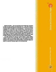
Figure 1. Schematic of the Ex-Situ Dissolution Approach (ESDA).

evaluation are missing from this study.21 The mixing tank that was employed by Burton is not practically required due to the presence of turbulent eddies within the pipeline and/or injection well.11,20,21 Zendehboudi et al. (2011) proposed a mathematical model to predict the CO2 droplet size versus time in a horizontal pipeline employed for the ESDA.20 The effect of gravity on mass transfer between the CO2 liquid droplets and the brine phase is investigated in this study for conditions whether the pipe is vertical or inclined. In addition to the role of mass transfer, it was found that the effect of pressure changes on the liquid droplet shrinkage is very important in this technology. Therefore, understanding these effects seems necessary to capture important aspects of the ESDA under turbulent flow conditions in the pipeline to injection well. The ESDA includes mixing of CO2 into brine along the pipeline and then injecting the mixture into the target formation. Since the CO2−brine system is hydrodynamically unstable, the liquid CO2 injected in the pipeline, with brine being the continuous phase, will break up into droplets in the brine phase. Understanding the behavior of a dispersed system is useful for the design and scaling up purposes. This is due to the fact that the interfacial area of droplets, physical properties of the ambient phase, and the flow regime affect the transport phenomena. In this paper, a formulation of mass transfer from suspended liquid CO2 droplets is presented. A mathematical expression is developed to estimate the droplet size along the pipeline prior to injection of the CO2−brine mixture into the target formation. Moreover, a quantitative analysis is conducted using experimental data available in the literature to validate the proposed mathematical model. Using an example, the droplet transport in the turbulent flow is demonstrated to examine the implementation and feasibility of the introduced methodology for geological sequestration of CO2. This paper also highlights the technical and economic feasibility of the ESDA in comparison with the standard CCS technologies. Important issues such as CO2 displacement, geochemical reactions, pressure build-up, well spacing, leakage of CO2, and dissolution efficiency are also addressed. Results from this study are presented and discussed in greater details throughout the paper.

2. THE EX-SITU CO2 DISSOLUTION PROCESS The Ex-Situ Dissolution Approach (ESDA) includes producing the brine from a saline aquifer, sparging CO2 into the brine phase in a pipeline with enough length to maintain a good mixing for CO2 dissolution, and then reinjecting the CO2-saturated brine into the saline aquifer.11,20 The described process reduces the risk of the buoyancy-driven leakage of CO2, due to the fact that CO2saturated brine has a slightly greater density than the in situ conditions brine. The proposed process is designed in a way that a CO2-rich phase will never exist as an immiscible with brine phase in the saline aquifer. This technique can be implemented for the large scale CO2 sequestration into saline aquifers at various depths.11,20,21 Unlike other CO2 sequestration techniques, it is possible to sequester notable amounts of CO2 in shallow and deep saline aquifers through this method, which allows more CO2 storage as a supercritical phase. Indeed, this is a significant advantage for the proposed technique over most of the common methods of massive CO2 sequestration, which are not efficient enough for CO2 sequestration in shallow formations.11,20,21 In theory, the proposed process meets the current regulations of the wastewater disposal. A schematic of the process is demonstrated in Figure 1. 2.1. Advantages of ESDA. The reduction of pressure buildup for a CO2 injection well is one of the benefits of using the ESDA technology. Safety regulations in the North America hinder injection rates to maintain the formation pressure below the overlying fracture pressure in order to avoid occurrence of leakage.4,12,13,21 Injection well pressure normally should not be over 80−90% of the estimated fracture pressure.4,12,13,15 Accurate control of this pressure build-up makes possible greater injection rates and thus a more effective CO2 sequestration scheme. Another operational advantage of the ESDA comes from lowering the CO2 leakage potential via abandoned wells when brine production is linked to large amount of CO2 injection. The CO2 leakage issue is central in oil and gas fields having many production wells. Another issue is related to the plume steering, where brine production is employed to influence the flow direction of the CO2 plume by changing the formation pressure.11−21 Efficient plume steering could have important 402


Energy & Fuels

Article

implications when possible remediation plans are considered in employing the ESDA. Last but not least, this new CO2 sequestration technique has a high potential to improve the storage capacity of the underground aquifer formation to store more CO2.

3. TECHNICAL AND SAFETY CHALLENGES IN CCS TECHNOLOGIES Issues such as CO2 injection, transportation, and leakage potential in CCS technologies are briefly described in this section with special reference on the ESDA technology. Geochemical reactions between rock and potential leakage pathways (e.g., fractures, faults, layer contacts) leading to alteration of well injectivity in the formation and increase in leakage potential are considered as a serious concern in CO2 sequestration techniques.4,12−15,21 Induced stress gradients due to injection result in the creation of new fractures or reactivation of existing fractures and faults. In addition, CO2 or resident brine leakage can affect the freshwater aquifers, unsaturated soil region, and the atmosphere.4,11−15,21 3.1. Important Parameters. There are a number of important parameters that affect the dissolution efficiency, capital cost, and power consumption of the ESDA technology. The main parameters include PVT of the fluid streams, injection and production flow rates, water salinity, selection of the EOS, wellbore expenses, and pipeline length.4,20,21 The contribution of each variable on target functions and uncertainty is independently examined. An artificial neural network (ANN) system combined with the particle swarm optimization (PSO) method was employed in this study to estimate the ESDA efficiency and storage capacity on the basis of the results presented in the literature via simulation runs. All of the above important variables were considered as input parameters for the ANN-PSO modeling. Through a trial and error technique, the optimal structure for the ANN-PSO system was determined to have one input layer (8 neurons), one hidden layer (10 neurons), and one output layer (2 neurons). After implementing training and testing phases, a reasonable match was observed between the literature data11,20,21 and predictive outputs, as shown in Figure 2. The contribution of each input parameter on the ESDA performance was obtained through employing a method suggested by Garson (1991)22 for connectionist weights. The relative significance of inputs, RI, was computed by eq 1. The higher correlation between any input variable and the output variable implied greater importance of the variable on the value of the dependent factor. n ⎡⎛ ivj ⎞ ⎤ ∑ j =H 1 ⎢⎜ ∑nv i ⎟Wj ⎥ ⎣⎝ k =1 kj ⎠ ⎦ RI = ⎤ ⎡ n n ⎡⎛ ivj ⎞ ⎤ ∑i =v 1 ⎢∑ j =H 1 ⎢⎜ ∑nv i ⎟Wj ⎥⎥ ⎣⎝ k =1 kj ⎠ ⎦⎦ ⎣

Figure 2. Real versus predicted ESDA performance for the ANN-PSO model: (a) training; (b) testing.

Figure 3. Relative impacts of main variables on the ESDA performance.

According to the PVT behavior of the CO2−brine system, it is common that an error of ±6 °C happens in predicting the temperature of the mixture. Temperature variation changes the amount of solubility and flow rate of required brine for the ESDA. The flow rate of brine significantly influences the operational and capital costs, and the energy consumption. Error percentage of ∼9% is reported between the experimental PVT data and the results obtained from the models developed by Duan and Sun (2003) and Spycher et al.(2003).20,21,23−26 The existing error definitely alters the thermodynamic status of the mixture, brine flow rate, energy expenditure, and capital expenses. Also, an error of ±4−8% is usually practical for salinity uncertainty.4,20,21,23−26 Such an alteration in salinity percentage affects brine flow rate, CO2 solubility, process design of the equipment, power consumption, and capital costs. Well design predictions for the injection and production wells vary for various regions and depths. Error in estimating well

(1)

Here, nH represents the number of hidden neurons, nv is the number of input neurons, ikj stands for the absolute value of input connection weights, and Wj is the absolute value of connection weights between the hidden and output layers. Figure 3 shows the relative importance of input variables on the target variables (e.g., ESDA performance). Temperature and injection flow rate, followed by pressure, were the most important parameters contributing in the ESDA CO2 sequestration. 403


Energy & Fuels

Article

high as three times more for the ESDA process compared to conventional CCS methods. Mineral precipitation in brackish water mixtures may happen as well, because the new ions and carbonic acid are introduced in the CO2−brine solution, and these reactions affect pH value, physical properties of solutions, and material properties.11,21 Furthermore, mineral precipitation in the pipeline, the injection/production wells, or the nearwellbore area of the porous medium alters the well injectivity.11,20,21 Moreover, the reactions between CO2, brine, and rock minerals can lower the injection rate by lowering the effective permeability of existing phases and intrinsic permeability of the target aquifers and/or formations. It is also a proven fact that the mineral dissolution in fractures impairs the effective fracture permeability. 3.5. CO2 Leakage. The driving forces for CO2 leakage generally are buoyancy force and pressure build-up due to fluid injection into the formation. The leakage occurs through faults, fractures, and active and/or abandoned wells. Leakage to shallower geological formations is a concern for drinking water resources contamination. Also, the leaked CO2 finally reaches the shallow subsurface area, resulting in high CO2 concentrations. This causes health and environmental risks at the ground surface.4−10,20,21,27 Assessment of such threats is an important factor in regulatory approval process and public acceptance. On the other hand, conducting health and safety evaluation is timeconsuming and costly. Several studies regarding CO2 injection and migration modeling associated with the leakage issue have been conducted.10,12−15,20,21,27 Employing the ESDA eliminates or minimizes leakage risks involved in CO2 sequestration technologies due to the nature of the processes involved. 3.6. Well Integrity. In principle, dealing with the mixture of brine and CO2 in large scale geological sequestration of CO2 into saline aquifers poses the risk of CO2 leakage through wells while applying any of CCS technologies. The CO2−brine mixture can lead to deterioration of well integrity through weakening of the cement, steel, and other materials used for well construction or casing such that the liquid solution lowers their strength, causing steel corrosion, and increases the cement permeability, resulting in fracturing and creating a passage-way for CO2 to leak.28,29 Thanks to many decades of oil industry experience in CO2 EOR, a basic knowledge is already available to tackle this issue during large scale geological sequestration of CO2.28,29 There are special cements available commercially that have high resistance in acidic environments and for high temperatures.29−31 However, using such materials may increase the cost of well construction and completion. Corrosion resistant materials such as 314 stainless steel and Hastelloy, along with casing corrosion prevention techniques, are now widely used, especially in the U.S.29−31 This technological advancement can be used in large scale geological CO2 sequestration practices to enhance the well integrity through lessening the risk of CO2 leakage when dealing with such corrosive mixtures. 3.7. CO2 Monitoring. CO2 monitoring is a crucial process during and after CO2 storage. Reservoir simulations and geophysics investigations are taken into account as two main approaches to monitor the CO2 flow in the underground formations.5,27 Running modeling simulations provides beneficial information on how is the CO2 distribution in the subsurface porous medium during and after storing CO2. Regional, crosswell, and/or single well mapping of CO2 phase are provided by geophysics measurement tools including seismic, electrical, and gravity measurement methods. The success of the geophysical measurements is dependent on a number of parameters such as

expenses strongly affects the capital costs and may cause a significant change while selecting a proper CCS technology. An error of ±50 to 150 m usually occurs when calculating pipeline length required for full dissolution of CO2 into the brine. Such an uncertainty influences the sequestration performance and the operational and capital expenses of the ESDA. The uncertainty of the injection/production rate is often in the range ±250 000−300 000 tonnes per year per well.11,20,21 The error in the prediction of injection rate, well spacing, and number of wells and pumps required for injecting brine affects project footprint, breakthrough phenomenon, and operational and capital costs. 3.2. PVT Behavior of CO2−Brine Mixture. Proper modeling of the CO2 sequestration in underground saline aquifers necessitates a precise PVT model. Acceptable predicted data for the thermodynamic and transport characteristics of brine and CO2 are very essential for estimating the CO2 solubility and storage capacity of sedimentary basins while employing various CO2 sequestration technologies such as ESDA. The thermodynamic behavior of CO2−brine at equilibrium condition has been addressed broadly in the literature. In this paper, the Duan and Sun (2003)25 and Spycher et al. (2003)26 PVT models are used to obtain component compositions at various temperatures and pressures while running simulation programs to calculate pressure build-up and well spacing. However, bubbly turbulent flow exhibits nonequilibrium conditions and phase transition in some parts of the pipeline (e.g., entrance length) over the ESDA. Having these conditions, the PVT data computation results in convergence issues and output reliability issues. Thus, the thermodynamic properties obtained from the simulation runs may not have a reasonable accuracy. This drawback implies the need of a sophisticated compositional simulator that includes an appropriate Equation Of State (EOS), such as modified Peng− Robinson, for modeling of transport and thermodynamics phenomena involved in the ESDA. 3.3. CO2 Displacing Brine. Besides the uncertainties in numerical and analytical modeling, some concerns for the ESDA are similar to those experienced in EOR processes. Injecting a huge amount of brine into an aquifer during a certain period of time is comparable with waterflooding operations in the oil reservoirs. The main problems for waterflooding operations include early water breakthrough, channeling, sweep efficiency, and viscous fingering effects.4,11,20,21 Similar problems for the ESDA dealing with the CO2−brine mixture are anticipated, while more complicated issues still remain unresolved about multiphase flow in porous media, particularly heterogeneous porous media.11,20,21 It is believed that a line-drive well configuration permits much flexibility in regulating injection and production flow rates such that a uniform fluid displacement is made in a proper manner.21 As hydrodynamic dispersion is a vital feature in EOR projects, onset of diluted CO2−brine mixture at the brine production wells (CO2 breakthrough in the brine producing well) returns CO2 to the ground, leading to performance reduction of the CCS plant and finally the operation shutdown.21 3.4. Geochemical Reactions and Carbonic Acid. When CO2 is dissolved in brine, the formation of carbonic acid takes place. The carbonic acid is reactive toward process elements such as pipeline, valves, seals, cement, and injecting wells in the ESDA technology.4,11,20,21 Therefore, precise safety considerations for equipment design, surface facilities, and injection/production wells are essential. Considering the cost of various materials, the costs for the apparatus and required wells will increase significantly, such that the equipment price might become as 404


Energy & Fuels

Article

In this section, the well spacing for the ESDA is computed at CO2 breakthrough. To do this, the breakthrough time is set for 50 years, while the porosity and permeability are assumed to be 20% and 40 mD (40 × 10−15 m2), respectively. The flow rate is set at 1.05 Mt/y per well, and 20 well pairs were used for this purpose. Using the CMG (the Computer Modeling Group software), simulations for this system were run to calculate the well spacing in a 3-D model. In the CMG simulation program, a value for spacing between injectors is chosen first and then a value is obtained for well spacing between the producers. The program then moves to the next value of the spacing of injection well and calculates the new value for the spacing between production wells. Figure 4 shows the spacing between wells in terms of the formation thickness.

the difference between physical properties of CO2 and porous medium fluids, temperature and pressure of the fluids, pressure distribution, well spacing, injection configuration, and the lithology and structure of the basin. As it is clear from the above statement, such a monitoring procedure should be conducted for conventional CCS technologies where the bulk CO2 is injected into the formation. To do this, higher costs and massive amount of time are required, considering there are still uncertainties in the magnitudes of fluid and formation characteristics even if an extensive study is performed. Based on the physics of the ESDA, a main part of this monitoring process is not required and more attention is given to design of surface facilities and process engineering. 3.8. Uncertainty Analysis. Prior to implementation of a particular CO2 sequestration method, the impacts of formation type (e.g., homogeneous, heterogeneous, carbonate, or sandstone type aquifer), injection strategy, injection rate, fluid properties, and well spacing are normally studied on the process performance. In general, various 3-D simulation runs are carried out to investigate the above aspects. This kind of simulations is practical and desired; however, accurate geological and reservoir engineering data are needed to estimate CO2 sequestration performance and storage capacity that are key for economic and technical analysis. Various factors such as CO2 price, energy cost, operational expenses, drilling and completion costs, and discounted rate of project economics have a significant effect on project economics. Almost all of the cost elements involve a great degree of uncertainties and variabilities. One of the useful techniques is a combination of a comprehensive design of experiments and the response surface method to conduct a study for analyzing of uncertainties. Collecting reservoir parameters and economic factors is necessary to attain acceptable outputs from an uncertainty analysis study. Much effort in this area should be made for CCS technologies to achieve planned goals. The economic and technical burden of uncertainty analysis in CO2 sequestration is reduced considerably through employing the ESDA. 3.9. Single Well CCS. Safety procedures of drilling and also a study of remediation alternatives make impossible utilization of a single well to inject several Mt CO2/y into an underground formation while using a CCS technique.4,5,11,20,21,27,32 Many CCS research and demonstration plants consist of only a single well. Employing just one injection well for a particular formation causes a number of technical and public acceptance issues. For instance, if the initial plan faces a complication issue, a time period of 5−14 days might be required to finish drilling another injection well. This could be difficult as the CCS plant needs to be operating continuously. Furthermore, many uncertainties in the underground formation parameters, lack of accurate and sufficient geological data, and necessity of characterization and history matching are other drawbacks of using a single well injection plan. On the other hand, drilling of additional wells will add significant extra costs to the CO2 sequestration operations. 3.10. Well Spacing. Determination of well spacing is vital in the line-drive well configuration. If the injection well is drilled very close to the brine production well, it is expected that early breakthrough of the CO2 will happen; however, the injectivity is of a high value.11,20,21,32 The well interference problem will occur and this will lower the magnitude of injection rate when the well spacing is very short. The small swept area between the injection and production wells will lead to premature breakthrough, as well. Hence, the spacing between wells is necessary to be computed appropriately when employing the ESDA.

Figure 4. Injector/producer well spacing versus injector/injector spacing at various formation thickness (m).

As shown in Figure 4, for any formation thickness, there is a specific spacing for injectors after which the well spacing between the production and injection wells remains almost unchanged. This characteristic value decreases as the formation thickness increases. The optimum well spacing should be obtained based on the process design and cost estimates for all setup components involving in the ESDA such that both technical and economic optimum conditions are attained. Then, the minimum footprint of the ESDA can be determined. 3.11. Pressure Build-up for the ESDA. An appropriate calculation is presented here in order to evaluate the effect of brine production during the ESDA technique on pressure buildup, considering 3-D simulations and various well configurations (see Figure 5 for more information). This model includes constant pressures for production and injection wells. In addition, one boundary condition at infinity is taken into account for the simulation runs. A 3-D model appears to be more reasonable than the radial system for modeling the pressure build-up around an injector. As brine production is started, a cone of pressure drop will grow around the producer. Once joined with a brine−CO2 injector, a combined cone of pressure build-up will develop at this stage; a point in distance between the two wells will be at a constant pressure that does not vary with time. Applying an infinity condition and a fixed production rate and pressure, the simulation model considered here clearly depicts the effect of rings of brine producers during the ESDA. Based on five various 405


Energy & Fuels

Article

facilitates injection at a constant flow rate with a lower compression cost. 3.12. CO2 Dissolution Efficiency. One of the important parameters in evaluation of the ESDA is the dissolution efficiency (η), which can be defined as the ratio of the mass (volume) of dissolved CO2 because of ex-situ dissolution to the initial mass of injected CO2. During the standard CCS operations involving bulk injection of CO2 (e.g., 1.0 Mt CO2/y) without brine, 6.5% CO2 is dissolved during 20 years of CO2 injection and only an additional 1.5% dissolves over 300 years according to numerical simulations reported in the literature.11 However, with brine injection at a rate of 20 Mt/y flowing through the pipeline, over 95% CO2 is dissolved within about 165 s because of the convectiveturbulence mechanism (refer to the example presented in this study). Figure 5. Effect of pressure control space on the injector pressure for the ESDA compared with conventional method (no brine production) [Total injection rate: 21 Mt/y. Thickness: 150 m. Permeability: 40 mD. Porosity: 20%].

4. MASS TRANSFER ASPECTS In this section, mass transfer from CO2 droplets during the ESDA is examined mathematically. According to Zendehboudi et al. (2012),33 the following relationship is obtained to determine the evolution of CO2 droplets along the pipeline length during the ESDA.

simulation runs, time evolution of pressure for the injection well is presented in Figure 5; where the constant-pressure boundary of the injectors changes from 2 to 16 km. BT refers to breakthrough time in Figure 5. As expected, as the pressure boundary condition approaches to the injection well, the pressure reduction for the injecting well will be greater. The CO2 plume arrives at about 11.5 km after 50 years of injection when there is no brine production. Breakthrough is defined here as the onset of the CO2 plume at the position of the constant pressure boundary condition. Breakthrough of the CO2 occurs for boundary distances smaller than 12 km, in the case studied here. It is clear that such close patterns of the producers also offer the most declines in the pressure of the injection well. The practical trade-off between having an effect and preventing breakthrough calls for production plans with either a horizontal well or multiple vertical production wells could be taken into account when implementing the ESDA. However, even when the constant pressure boundary condition of the wells is at 12 km, the reduction in pressure is usually considerable above the 50 years time limit. As soon as any large pressure alterations move toward the constant pressure boundary, afterward, the pressure of injection well lowers, as depicted in Figure 5. At the beginning, no pure brine flow basically exists at the pressure external boundary because compressibility within the area is prevailing. As time proceeds, considerable brine flow rate happens through the boundary, improved by the fixed pressure boundary made by the producers. When this phenomenon takes place, the brine−CO2 phase is substituting the pure brine in the swept area. This leads to reduction of total resistance for fluid flow in the domain due to maintaining of higher driving force. It is evident from Figure 5 that the pressure build-up at the injection well can be controlled by brine production using the newly introduced ESDA technology. At 50 years, it can decrease the pressure of injection well by nearly 19% between the no production case (conventional approach) and the first option without occurrence of breakthrough. It should be mentioned here that the main restriction on injection rate is to keep the formation pressure constant due to the injection at less than the fracture pressure. At the injection well pressure, the reduction of transient pressure can give the potential for greater injection rates at later times. In addition, lowered pressure at the injector well

d(d p) dt +

d p ρBrine 3ρp

3⎤ ⎡ 2kϕ0 ⎢ ρp,0 ⎛ d p ⎞ ⎥ 2kCs ⎟⎟ =− + − ⎜⎜ 1 − ϕ0 ⎢⎣ ρp ρp ⎝ d p,0 ⎠ ⎥⎦

⎞ M wpU ⎛ f U 2 − g⎟ ⎜ ZavgRTavg ⎝ D 2 ⎠

(2)

where k is the mass transfer coefficient, Cs is the saturation concentration of CO2 on the droplet surface, ρp is the droplet density, ϕ0 is the initial volumetric fraction of CO2 in the mixture, ρBrine is the brine density, Zavg is the average compressibility factor, Mwp molecular weight of CO2 droplets, U is the average mixture velocity, Tavg is the average temperature of the mixture, f is the friction factor, and D is the pipe diameter. R and g are the universal gases constant and gravitational force, respectively. All the 0 in subscripts refer to the initial or inlet conditions. The Supporting Information presents the derivation of eq 2 in detail. 4.1. Mass Transfer Coefficient. It is very important in convective mass transfer of droplets to have an appropriate selection of the empirical correlations for Sh, defined as kdp/ DCO2−Brine. where DCO2−Brine is the diffusion coefficient for the CO2 in brine (refer to the Supporting Information for calculation of the diffusivity coefficient). Two groups of correlations are employed here alternatively. Assuming the CO2 droplet as a rigid sphere, the following equations can be used for fully turbulent regime: Ranz and Marshal (1952):34 Sh = 2 + 0.6Re 0.5Sc 0.33

(3)

Kress and Keyes (1973):35 ⎛ d p ⎞2 0.5 Sh = 0.34⎜ ⎟ Re 0.94 f Sc ⎝D⎠

(4)

Assuming the droplet as a fluid sphere with a tangentially mobile surface, the following correlation is found proper for the high values of Re:36−38 406


Energy & Fuels Sh =

Article

2 [1 − (2.89 + 2.15β 0.64 )Re−0.5]0.5 (ReSc)0.5 π

range of Reynolds number (Re).36 In the case of fully developed turbulent flow (e.g., high values of Re), the minimum stable droplet diameter can be estimated according to the following equation:36

(5)

where β denotes the CO2-to-water viscosity ratio. The rigid sphere approximation is basically suitable for hydrate-coated droplets. The approximation of fluid sphere is practical for hydrate-free droplets if their surface is free from any obstacles in their tangential motion, such as surfactant pollutants, or a mechanical droplet-holding device. It should be noted here that eq 5 appears to be more realistic for the case under study. Therefore, this equation substitutes eq 17 presented in our previous publication.20

d p,min =

6. OPERATING AND CAPITAL EXPENSES CO2 capture and compression are usually the most expensive stages of a CCS plant. The expense of these two steps is in the range of 50−80% of the CCS total cost, depending on the process and CO2 characteristics.41 CO2 transportation cost by pipeline varies between 0.5 and 7 $/t CO2 for different pipe materials and CCS processes.41,42 This cost is around 8−12% of the total cost of a typical CCS plant.5,21,27,41,42 The expenses of CO2 storage consist of drilling injection/production wells and pumping facilities. Depending on geologic characteristics, the sequestration cost is typically estimated to be 1−9 $/t CO2.42−44 The monitoring cost is usually lower than 0.1 $/t CO2.44−47 The main capital expenses for CO2 geological storage include drilling and construction of wells, surface facilities, and plan management. The operating expenses also come from maintenance, fuel, and manpower costs. The costs for site selection, licensing, and reservoir characterization are estimated to be $1.685 million for saline aquifers.21,45−47 The capital, operating, and site characterization expenses are about 0.5 $/t CO2 for CO2 storage in onshore saline formations.45−48 This estimate does not include the expenses for monitoring, remediation, and long-term liabilities. The costs for basic and advanced monitoring packages are in the ranges 0.04−0.05 and 0.069−0.085 $/t CO 2 , respectively, for a 50-year CO 2 sequestration process in saline aquifers.45−48 Number of wells, well spacing, well expenses, and cost of ground and underground CCS facilities are functions of CO2 sequestration type, depth, and formation characteristics. The well cost is a major component in the storage part. Each single well costs around $ 200 000 for onshore plants; however, this cost for offshore horizontal wells may increase to $ 25 million.47,48 It should be also noted that the cost of well integrity monitoring is assumed to be about $15 million, considering injection/production wells with depth of 7500 ft.47,48 In addition to CCS costs mentioned above, IPCC (2011) reports the following bottom-up cost estimates for CCS plants to sequester CO2 in geological formations:49 (1) The total cost of CCS technology in power plants varies from 40 to 80 $/t CO2.49 (2) The cost for capturing CO2 from a coal and/or gas fired plant varies between 30 to 60 $/t CO2.49 (3) Transportation section costs in the range of 1−8 $/t CO2.49

(6)

where dp,max is the maximum stable droplet diameter in a turbulent flow of intensity ε,̅ and ρc and σ are the density and interfacial tension of the continuous phase, respectively. Sleicher (1962) carried out experiments on break up in a turbulent pipe flow and concluded that the assumption of homogeneous isotropic turbulence is only applicable in the core of the pipe, not in the area where break-up takes place. Hence, eq 6 cannot be used to determine dp,max in a turbulent pipe flow.40 Sleicher (1962) proposed a semiempirical correlation that takes into account effect of the dispersed phase viscosity, μd:40 d p,max ρc U 2

μc U

σ

σ

⎡ ⎛ μ U ⎞0.7 ⎤ = 38⎢1 + 0.7⎜ d ⎟ ⎥ ⎝ σ ⎠ ⎥⎦ ⎢⎣

(8)

where E is an empirical constant and ρd is the density of the dispersed phase. According to the values of minimum and maximum stable droplet diameters, a wide range of initial droplet sizes is now available to find out the effect of droplet size on the mass transfer during ex-situ dissolution process. The correlations employed in this paper for estimation of minimum and maximum stable sizes have higher accuracy and applicability for the bubbly flow in vertical pipelines compared to the relationships defined in our previous work.20,33,36−40

5. MAXIMUM AND MINIMUM STABLE DROPLET SIZE Finding the minimum and maximum stable sizes of droplets, break-up or/and coalescence frequency, and droplets size distribution is essential in characterization of break up and coalescence mechanisms during bubbly flow processes such as ESDA.36−38 Surface tension and dynamic forces are the two main forces that apply to droplets or bubbles in a turbulent flow with dispersion. The theoretical basis to assess stable droplet sizes is based on the balance between these forces (e.g., Levich, 196236). This balance dictates the values of minimum and maximum stable diameter of the droplets flowing in a bubbly turbulent flow. Also, it should be noted here that the size of pores in a sparger, usually employed in the bubbly flow regime, can affect droplet size distribution between these two specific diameter sizes but does not change the magnitudes of those characteristic sizes considerably. Identification of the maximum droplet diameter (dp,max) that opposes breakup in a turbulent flow regime is a well-addressed subject in the literature.36−38 However, this is meant to be used for cases that often occur in industrial pipe flows. Some researchers have related dp,max with the Sauter mean diameter, which is frequently employed as a measure of available specific surface area in dispersions.36−40 Hinze (1955) proposed the following empirical expression based on experimental data for the maximum stable size of droplets:39 ⎛ ρ ⎞3/5 d p,max ⎜ c ⎟ ε ̅ 2/5 = 0.725 ⎝σ ⎠

1 ⎛ U2 ⎞ E⎜ ⎟(ρ ρ2 )1/3 3 ⎝ σ ⎠ c d

(7)

where U is the mean velocity in the pipe. Equation 7 is valid for the viscosity range 0.3 mPa·s < μd < 30 mPa·s.40 Similarly to breakup, coalescence has also been associated with a characteristic droplet size, the minimum droplet diameter, dp,min, that can resist coalescence. For the calculation of the minimum stable size of the droplets, Levich (1962) suggested different expressions, depending on the 407


Energy & Fuels

Article

(4) Expenses for CO2 storage and its monitoring and verification vary between 5 and 10 $/t CO2, depending on various factors such as number of wells, type of formation, and so on.49 Comparing ESDA with conventional CCS methods, careful consideration in selecting pipeline and pumps materials is required for the ESDA. Table 1 shows the appropriate materials along with their costs for various fluids contributing in CO2 sequestration processes. Table 1. Proper Materials and Their Costs for the Fluids in the ESDA50,51 fluid

material

price

brine

304 stainless steel and/or 314 stainless steel

CO2 (dry)

carbon steel

CO2 (wet)

304 stainless steel

carbonic acid

304 stainless steel and/or 440 stainless steel

pipeline: 2800−3500 $/t pump: 40 000−80 000 $/set pipeline: 750 $/t pump: 10 000−30 000 $/set pipeline: 2800−3500 $/t pump: 40 000−80 000 $/set pipeline: 2800−3500 $/t pump: 40 000−80 000 $/set

As shown in Table 1, a significant reduction in equipment price is observed for conventional CCS technique compared to the ESDA if CO2 fluid is free of water prior to injection into the formation. This case is uncommon in CCS processes, since CO2 mostly contains water from previous stages such as its capture. According to the cost estimates reported in this section, IEAGHG (2007) and Burton (2008),20,21,41−52 the operating (OPEX) and capital (CAPEX) expenditures for the ESDA process in saline aquifers are given in Figure 6, if average values of the costs for CCS elements are used in the economical calculation. The OPEX in terms of the power plant is ∼49% of the power output, and the CAPEX is about $955 000 per MW of the power plant.20,21,41−52 For a power plant with an output of 1000 MW, about 490 MW is required to operate the capture and compression processes. Also, the CAPEX estimated for this case would be around $955 M. It is important to note that all costs are adopted for year 2012. Based on the estimates presented in Figure 6, and the costs for conventional techniques (as shown in Figure 7), the ESDA technique has greater OPEX compared with the standard processes by about 9% of the power plant output. As depicted in Figure 7, the new CO2 sequestration method proposed in this study decreases the costs of project monitoring and remediation by up to 65%. It is also seen that the ESDA has higher CAPEX than the standard processes because of an additional 57% of total cost required for running an ex-situ dissolution plant. Although the ESDA is more expensive than other processes that deal with injection of bulk CO2 into saline aquifers, the higher dissolution efficiency obtained through using this technique minimizes the risk of CO2 leakage risks and increases the formation capacity that can be available to store CO2.

Figure 6. OPEX (a) and CAPEX (b) for ESDA.

suitable CCS technique, since this formation, which is a part of the Michigan and Appalachian basins, is located in southwestern Ontario.53−55 As this aquifer consists of various regions with different depths that are either greater than 800 m or less, the ESDA process can be employed safely to sequester CO2, even into the areas that have a permeable caprock and/or a shallow depth. This advantage allows installing the capture facility as close as possible to the power plants, leading to cost reduction for capture and transportation stages. Thus, it can compensate a part of extra expenses that are required to run the ESDA process compared to the conventional CCS techniques. On the other hand, the ESDA offers an efficient CO2 sequestration process with lower leakage risks and a higher storage capacity for Mt. Simon aquifer. However, further technical and economic investigations are required prior to implementation of this new technology for saline aquifers (e.g., Mt. Simon) in Canada and U.S.A.

8. CASE STUDY Efficiency of the proposed method is examined employing a case study in real scale. Suppose that liquid CO2 from a cylinder and a brine stream are introduced into a pipeline. The purity of the liquid CO2 is assumed to be 100%. The brine phase and CO2 are at a desired temperature equal to 20 °C, and the input pressure is 70 bar. The flow rate of the high-pressure saline water is 20 Mt/y and the volumetric fraction of CO2 is about 5% in the mixture.

7. APPLICATION OF THE ESDA IN ONTARIO, CANADA The Nanticoke generation plant and other power plants situated around Sarnia, Ontario, Canada, are producing more than 20 Mt CO2/y.53−55 To mitigate such a large amount of CO2 emissions, the Mt. Simon sandstone formation as a saline aquifer could be an appropriate candidate for CO2 sequestration through a 408


Energy & Fuels

Article

Figure 9. Droplet size versus time at two different initial sizes for a specific correlation of the Sherwood number (Sh = 2).

Figure 7. OPEX (a) and CAPEX (b) for conventional CCS technique versus ESDA.

Using a numerical technique, the volumetric flow (Q) of the brine phase was considered 0.665 m3/s in a pipeline with diameter (D) of 0.15 m. The inner turbulence scale (I ∝ 5.3DRef−3/4) in this case is obtained equal to 0.002 mm. As the Reynolds number for the above parameters is high (e.g., Re = 23 400 000), the differences in Sherwood numbers calculated by using different relationships would be very significant. The variations of the diameter of a single CO2 droplet during the time period t = 1500 s for four different initial droplet sizes dp = 0.02, 0.002, 0.0002, and 0.000002 m are shown in Figures 8, 9 and 10. It should be noted here that the droplet behavior changes considerably, depending on whether the Sherwood number is given by eq 4 or eq 5 or Sh = 2. Therefore, the results obtained

Figure 10. Droplet size versus time according to eq 5.

using eq 4 are presented in Figure 8, while Figures 9 and 10 depict the droplet evolution while employing Sh = 2 and eq 5, respectively. Since the mass transfer rate in the case of eq 5 is very high, the size of the droplets decreases. It should be mentioned here that the smallest droplets considered here (dp = 0.000002) were completely dissolved at the length of lower than 100 m. In general, the smaller the droplet size the stronger its tendency to be dissolved. The main reason is that smaller droplets are characterized by higher specific rate of the CO2 dissolution compared with the larger droplets. The change in droplet size for an upward pipe is the result of two competing factors: (i) CO2 mass transfer to the ambient brine that causes droplet shrinkage and (ii) the pressure drop expands the droplets in terms of size. Equation 4 and Sh = 2, in contrast to eq 5, exhibit the low mass transfer rates, leading to the droplet growth for any initial droplet size if the injection well is located at upper level with respect to the ground level of the CO2 capture facilities. However, an increase is observed in pressure along the pipe length due to the hydrostatic pressure, while injecting the CO2−brine mixture into the well. Thus, an increase in both pressure and mass transfer rate accelerates the droplet shrinkage.

Figure 8. dp/dp,0 versus time based on eq 4. 409


Energy & Fuels

Article

The impact of the CO2 volume fraction on the droplet size evolution is demonstrated in Figure 11, based on eq 5. As one can

Figure 11. Droplet size versus time at various CO2 hold-ups.

see from Figure 11, the mass transfer drops dramatically as the CO2 hold-up increases. Rates of the droplet size change having initial diameter dp = 0.002 m with different initial CO2 hold-ups (ϕ0 = 0.01, 0.05, 0.08, and 0.1) are compared. According to eq 5, the CO2 hold-up causes an increase in the average concentration of the CO2 dissolved in the ambient brine. As a result, the difference in concentrations between the droplet boundary and the ambient brine becomes smaller, resulting in a lowered mass transfer. The results obtained based on eq 5 clearly demonstrate the influence of the CO2 volume fraction as the droplet size varies versus time at any ϕ0. In addition, the rate of diameter change slightly increases by increasing the CO2 hold-up. Figure 12 presents a comparison between horizontal and vertical pipelines with respect to the efficiency of the exdissolution methodology for three different Sh correlations. If the vertical case is supposed to be downward, then a full dissolution occurs within the pipe length of 1120, 250, and 220 m according to eqs 3, 4, and 5, respectively. The required lengths for complete dissolution of the CO2 in a horizontal pipe are 1530 and 450 m in the worst and best cases, respectively. The main reason for such a large difference between vertical and horizontal cases is the strong effect of pressure increase on droplets shrinkage for the vertical downward pipe. It should be noted here that if the pipe goes uphill, full dissolution would happen in a longer length compared with that for downward pipe and even horizontal cases. This is because the pressure reduction causes growth in the volume of droplets. According to Figure 12, it can be concluded that when the mass transfer coefficient increases, the effect of potential energy on the droplet shrinkage decreases. This leads to a difference between the dissolution behaviors of droplets flowing through a vertical pipe. A lower difference was observed for eq 5 compared with eqs 3 and 4. This is due to the fact that eq 5 predicts higher value for mass transfer coefficient when the bubbly turbulent dissolution is established in the process. Although the mass transfer phenomenon is more dominant in size reduction of the droplets within a vertical pipeline undergoing a fully turbulent flow, increasing pressure that happens along a downward pipe enhances droplet shrinkage, basically. Thus, the model developed here enables analyzing the droplet behavior if a proper correlation for the mass transfer is known. To quantify the effects of pressure difference and mass transfer on the droplet shrinkage, Figure 13 is plotted. It is obvious from the figure that the effect of pressure on droplet shrinkage increases as the CO2

Figure 12. Droplet diameter versus time during the ESDA for vertical and horizontal pipes, (a) eq 3, (b) eq 4, and (c) eq 5.

droplets move forward and approach to the end point of the pipeline. Although the effect of pressure change is small compared to that of mass transfer on the droplet shrinkage, this factor affects the droplet volume considerably when the pipeline is long enough or the saline aquifer is deep (e.g., height or length >1000 m). In addition, Figure 13 shows that no significant change in the droplet size is observed and the mass transfer driving force tends to diminish when the droplet volume becomes very small. This condition corresponds to a fairly long time duration that the CO2 droplets are in touch with the brine phase. In this case, the effects of both parameters remain almost constant as the mixture goes down along the pipeline or well length. This numerical example also indicates that the uncertainty in the Sherwood number caused by the absence of conclusive data 410


Energy & Fuels

Article

9. CONCLUSIONS The following seven key conclusions can be drawn based on the results of this study: (1) The brine flow rate, liquid CO2 hold up, pipeline orientation, and PVT behavior of the mixture affect droplet size and, consequently, the shrinkage of the liquid CO2 droplets during the ESDA. The ANN-PSO technique showed that the mixture temperature and flow rate have the highest impacts on the ESDA performance (2) A numerical method was employed to predict the droplet size along a pipeline when a bubbly flow regime is established for a turbulent dispersed system. (3) In a diffusion-dominated system, about 70% of the CO2 phase becomes dissolved in a pipe with 3000 m length, whereas almost full dissolution will occur in the convective dominant systems such as the ESDA if the same pipe length is employed. (4) The numerical example presented here showed that it is technically feasible to attain full dissolution of CO2 into the brine stream along the injector before the CO2 − brine mixture arrives at the underground aquifer. (5) The variation in droplet size results from two opposing features: mass transfer from the CO2 droplets to the ambient brine phase leading to the droplet shrinkage and pressure drop causing the CO2 droplet growth. Therefore, total pressure change for a downward vertical pipe enhances the droplet shrinkage. (6) The ESDA provides obvious advantages in terms of pressure management in the target formation through brine production. The brine production also minimizes the water requirements for the operation. (7) The ESDA is a practical technique for CO2 sequestration in saline aquifers at a wide range of depths. Estimations of capital expenses per tonne of CO2 stored indicated that the ESDA is about 57% more expensive than the standard techniques; however, the new process has much higher dissolution efficiency, and it is much safer with respect to leakage issue.

Figure 13. Contribution of mass transfer and pressure in CO2 droplet shrinkage based on eq 5.

for the case of pipeline flow inhibits reliable assessment of the droplets behavior under the conditions of pressure drop or increase. It should be mentioned here that the stratification effect and/ or slip effect between the liquid (ambient phase) and droplets is considered for upward and downward vertical fluid bubbly flow in order to calculate the mixture velocity and pressure drop. In this case study, the contribution of slip effect was considered while calculating pressure drop along the pipeline in the first runs of the MATLAB program; however, no considerable difference was observed in terms of the pressure drop, and the ESDA performance compared to the case that no slip flow was assumed. The main reason is that the brine−CO2 mixture is a dilute solution that contains just 5% CO2 during the ESDA process. It was found here that it is technically feasible in practical cases to have complete dissolution of CO2 into the brine phase along the injection well before the mixture reaches the formation. Hence, a CO2 capture facility can be established in the vicinity of the injection well in the ESDA and the horizontal pipeline or mixing tank for premixing under turbulent conditions is no longer needed. It is important to note that the ratio (dp/dp,0) in this example was directly related to the percentage dissolution of CO2 droplets (see point no. 3 in the Conclusions). This assumption is erroneous if a high concentration of CO2 exists in the brine phase and the entrance length of the pipeline with transition state is the pipe element under study. However, the concentration of CO2 in brine is almost 5% in the real cases undergoing the ESDA; thus, the possibility of coalescence occurrence is low. Number of the droplets can be also considered constant, since this study is dealing with the developed pipeline flow. It should be noted here that the assumption appears to be acceptable for dilute bubbly solutions, while it is incorrect because of presence of breakage and coalescence phenomena while using concentrate CO2−brine mixture. Further research is necessary in order to address the different aspects of the ESDA before its field implementation for largescale geological sequestration of CO2. Research projects are underway to address the interaction between CO2 droplets (e.g., break-up process) and also assess economic feasibility of the ESDA with more details.

■

ASSOCIATED CONTENT

S Supporting Information *

Derivation of the mass transfer governing equation (e.g., eq 2) and the proper correlations to calculate important parameters such as diffusion coefficient and CO2 solubility in brine. This information is available free of charge via the Internet at http:// pubs.acs.org/.

■

AUTHOR INFORMATION

Corresponding Author

*E-mail: [email protected]. Notes

The authors declare no competing financial interest.

■

ACKNOWLEDGMENTS The authors acknowledge the Mitacs Elevate and Natural Sciences and Engineering Research Council (NSERC) of Canada for financial support of this study.

■

NOMENCLATURE

Acronyms

ANN = artificial neural network 411


Energy & Fuels

Article

ϕ = CO2 hold-up v = μ/ρ = kinematic viscosity of liquid, (m2/s) α = salting-out coefficient β = CO2-to-water viscosity ratio Δ = difference operator ε = energy dissipation per unit mass in turbulent stream, (m2/ s3) η = dissolution efficiency ρ = density of fluid, (kg/m3) ρBrine = density of brine, (kg/m3) ρp = density of CO2 droplet, (kg/m3) σ = surface tension, (N/m)

BT = breakthrough time CAPEX = capital expenditures CCS = carbon capture and storage CMG = computer modeling group cte = constant EOS = equation of state IEAGHG = International Energy Agency Greenhouse Gas ESDA = Ex-Situ Dissolution Approach IPCC = Intergovernmental Panel on Climate Change OPEX = operational expenditures PSO = particle swarm optimization PVT = pressure−volume−temperature

Subscripts

Variables 2

A = surface area of droplet, (m ) a, b, c = arbitrary constants defined in the paper C = concentration of CO2, (kg/m3) C∞ = CO2 concentrations in brine, (kg/m3) Cs = CO2 concentrations at the droplet-liquid interface, (kg/ m3) D = pipe diameter, (m) DCO2−Brine = diffusivity of CO2 in brine, (m2/s) or (cm2/s) DCO2−W = diffusivity of CO2 in water, (m2/s) or (cm2/s) dm/dt = mass flux on droplet boundary, (kg/s) dp = droplet diameter, (m) f = friction factor g = acceleration due to gravity, (m/s2) I ∝ 5.3DRef−3/4 = inner turbulence scale, (m) ikj = absolute value of input connection weights k = coefficient of mass transfer, (m/s) L = pipeline length, (m) m = mass, (kg) Mw = molecular weight, (kg/kg.mol) nH = number of hidden neurons nv = number of input neurons P = pressure, (Pa) or (bar) Q = volumetric flow rate, (m3/s) R = gases constant, (j/gmol.K) r = spherical coordinate Rb = solubility of CO2 in brine, (mol/cm3) RCell = cell radius, (m) Ref = UD/v = Reynolds number based on pipe diameter Rep= Udp/v = Reynolds number based on droplet diameter RI = relative importance in eq 1 Ro = roughness of pipe, (m) Rp = drop (droplet) radius, (m) RW = solubility of CO2 in water, (mol/cm3) S = salinity in weight percent, % Sc = v/DCO2−Brine = Schmidt number Sh = kdp/DCO2−Brine = Sherwood number T = temperature, (°C) or (K) t = time, (s) tmax = residence time of droplet in pipeline, (s) U = average flow velocity, (m/s) VCell = cell volume, (m3) VL = liquid volume in a cell, (m3) Vp = CO2 droplet volume, (m3) Wj = absolute value of connection weights x = x-axis Z = compressibility factor

■

avg = average c = continuous Cell = droplet cell d = dispersed f = fluid L = liquid max = maximum min = minimum 0 = inlet (initial) pipe conditions p = droplet S = surface W = water

REFERENCES

(1) Marchetti, C. On geoengineering and the CO2 problem. Climate Change 1977, 1 (1), 59−68. (2) Halmann, M. M.; Steinberg, M. Greenhouse Gas Carbon Dioxide Mitigation; Lewis: Boca Raton, 1999. (3) Herzog, H. J. What future for carbon capture and sequestration. Environ. Sci. Technol. 2001, 35 (7), 148A−153A. (4) Burton, M.; Bryant, S. L. Eliminating buoyant migration of sequestered CO2 through surface dissolution: Implementation costs and technical challenges. SPE Reservoir Eval. Eng. 2009, 12 (3), 399−407. (5) Intergovernmental Panel on Climate Change (IPCC). Climate Change: The Physical Science Basis; Cambridge University Press: Cambridge, 2007. (6) Eccles, J.; Pratson, L.; Newell, R. G.; Jackson, R. B. Physical and economic potential of geological CO2 storage in saline aquifers. Environ. Sci. Technol. 2009, 43, 1962−1969. (7) Liu, B.; Zhang, Y. CO2 modeling in a deep saline aquifer: A predictive uncertainty analysis using design of experiment. Environ. Sci. Technol. 2011, 45, 3504−3510. (8) Benson, S. M.; Myer, L. Monitoring to ensure safe and effective geologic storage of carbon dioxide. Intergovernmental Panel on Climate Change (IPCC) Workshop on Carbon Sequestration, Regina, Saskatchewan, Canada, Nov., 2002. (9) Keith, D. W.; Hassanzadeh, H.; Pooladi-Darvish, M. Reservoir engineering to accelerate dissolution of stored CO2 in brines. 7th International Conference on Greenhouse Gas Control Technologies, IEA Greenhouse Gas Program, Cheltenham, U.K., 2004. (10) Dentz, M.; Tartakovsky, D. M. Abrupt-interface solution for carbon dioxide injection into porous media. Trans. Porous Media 2009, 79, 15−27. (11) Leonenko, Y.; Keith, D. W. Reservoir engineering to accelerate the dissolution of CO2 stored in aquifers. Environ. Sci. Technol. 2008, 42, 2742−2747. (12) Nordbotten, J. M.; Celia, M. A.; Bachu, S. Injection and storage of CO2 in deep saline aquifers: analytical solution for CO2 plume evolution during injection. Trans. Porous Media 2002, 58, 339−360. (13) Little, M.; Jackson, R. Potential impacts of leakage from deep CO2 geo-sequestration on overlying freshwater aquifers. Environ. Sci. Technol. 2010, 44, 9225−9232.

Greek Letters

μ = dynamic viscosity, (mPa·s) ≈ = sign of proportionality 412


Energy & Fuels

Article

(14) Pau, G. S. H.; Bell, J. B.; Pruess, K.; Almgren, A. S.; Lijewski, M. J.; Zhang, K. High-resolution simulation and characterization of densitydriven flow in CO2 storage in saline aquifers. Adv. Water Res. 2010, 33 (4), 443−455. (15) Bruant, R. G.; Celia, M. A.; Guswa, A. J.; Peters, C. A. Safe storage of CO2 in deep saline aquifers. Environ. Sci. Technol. 2002, 36 (11), 240A−245A. (16) Hassanzadeh, H.; Pooladi-Darvish, M.; Keith, D. W. Stability of a fluid in a horizontal saturated porous layer: Effect of nonlinear concentration profile, initial, and boundary conditions. Trans. Porous Media 2006, 65, 193−211. (17) Adams, J. J.; Bachu, S. Equations of state for basin geofluids: Algorithm review and intercomparison for brines. Geofluids 2002, 2 (4), 257−271. (18) Riaz, A.; Hesse, M.; Tchelepi, H. A.; Orr, F. M. Onset of convection in a gravitationally unstable diffusive boundary layer in porous media. J. Fluid Mech. 2006, 548, 87−111. (19) Seto, C. J.; McRae, D. G. Reducing risk in basin scale CO2 sequestration: A framework for integrated monitoring design. Environ. Sci. Technol. 2011, 45, 845−859. (20) Zendehboudi, S.; Khan, A.; Carlisle, S.; Leonenko, Y. Ex-situ dissolution of CO2: A new engineering methodology based on mass transfer perspective for enhancement of CO2 sequestration. Energy Fuels 2011, 25 (7), 3323−3333. (21) Burton, M. Surface dissolution: Addressing technical challenges of CO2 injection and storage in brine aquifers. M.Sc Thesis, The University of Texas at Austin, 2008. (22) Garson, G. D. Interpreting neural-network connection weights. Artificial Intelligence Expert 1991, 6, 47−51. (23) U.S. Environmental Protection Agency (U.S. EPA). Determination of maximum injection pressure for class I wells. United States Environmental Protection Agency Region 5−Underground Injection Control Section Regional Guidance #7; U.S. EPA: Washington, DC, 1994. (24) Hangx, S. J. T. Behaviour of the CO2−H2O system and preliminary mineralisation model and experiments. CATO Work Package 188, WP 4.1; Shell International E&P: Houston, TX, 2005. (25) Duan, Z.; Sun, R. An improved model calculating CO2 solubility in pure water and aqueous NaCl solutions from 273 to 533 K and from 0 to 2000 bar. Chem. Geol. 2003, 193, 257−271. (26) Spycher, N.; Pruess, K.; Ennis-King, J. CO2−H2O mixtures in the geological sequestration of CO2. I. Assessment and calculation of mutual solubilities from 12 to 100 °C and up to 600 bar. Geochim. Cosmochim. Acta 2003, 67 (16), 3015−3031. (27) Intergovernmental Panel on Climate Change (IPCC). Special Report on Carbon Dioxide Capture and Storage; IPCC: Geneva, Switzerland, 2005. (28) Watson, T. L.; Bachu, S. Evaluation of the potential for gas and CO2 leakage along wellbores. E&P Environmental and Safety Conference, Galveston, TX, March 5−7, 2007; SPE 106817. (29) Moritis, G. SWP advances CO2 sequestration, ECBM, EOR demos. Oil Gas J. 2008, 106 (37), 60−63. (30) Meyer, J. P. Summary of carbon dioxide enhanced oil recovery (CO2 EOR) injection well technology. API Special Rep. 2008, 62. (31) Barlet-Gouédard, V.; Ayache, B.; Rimmelé, G. Cementitious material behavior under CO2 environment: A laboratory comparison. 4th Meeting of the Well Bore Integrity Network, Paris, France, March 18− 19, 2008. (32) Buscheck, T. A.; Sun, Y.; Hao, Y.; Wolery, T. J.; Bourcier, W.; Tompson, A. F. B.; Jones, E. D.; Julio Friedmann, S.; Aines, R. D. Combining brine extraction, desalination, and residual-brine reinjection with CO2 storage in saline formations: Implications for pressure management, capacity, and risk mitigation. Energy Proc. 2011, 4, 4283− 4290. (33) Zendehboudi, S.; Leonenko, Y.; Shafiei, A.; Soltani, M.; Chatzis, I. Modeling of CO2 droplets shrinkage in ex situ dissolution approach with application to geological sequestration: Analytical solutions and feasibility study. Chem. Eng. J. 2012, 197, 448−458. (34) Ranz, W. E.; Marshall, W. R. Evaporation from drops. Chem. Eng. Prog. 1952, 48 (3), 141−146.

(35) Kress, T. S.; Keyes, J. J. Liquid phase controlled mass transfer to bubbles in co-current turbulent pipeline flow. Chem. Eng. Sci. 1973, 28, 1809−1823. (36) Levich, V. G. Physicochemical Hydrodynamics; Prentice-Hall: Englewood Cliffs, NJ, 1962. (37) Clift, R.; Grace, J. R.; Weber, M. E. Bubbles, Drops, and Particles; Academic Press: New York, 1978. (38) Nigmatulin, R. I. Dynamics of Multiphase Media; Hemisphere Publication Corporation: New York, 1991. (39) Hinze, J. O. Fundamentals of the hydrodynamic mechanism of splitting in dispersion processes. AIChE J. 1955, 13, 289−295. (40) Sleicher, C. A. Maximum stable drop size in turbulent flow. AIChE J. 1962, 8 (4), 471−477. (41) Carbon Capture: Beyond 2020; U.S. Department of Energy (DOE): Gaithersburg, MD, 2010. (42) McCoy, S.; Rubin, E. An engineering-economic model of pipeline transport of CO2 with application to carbon capture and storage. Int. J. Greenhouse Gas Control 2008, 2 (2), 219−229. (43) McCoy, S. The economics of CO2 transport by pipeline and storage in saline aquifers and oil reservoirs. Carnegie Mellon University, Pittsburgh, 2008. (44) McCoy, S.; Rubin, E. Variability and uncertainty in the cost of saline formation storage. Energy Proc. 2009, 1 (1), 4151−4158. (45) Benson, S. M. From a geological perspective. Third Annual Conference on Carbon Capture and Sequestration; VA Monitor Exchange Publications: Alexandria, VA, 2004. (46) Benson, S. M. Lessons learned from industrial and natural analogs for health, safety, and environmental risk assessment for geologic storage of carbon dioxide. Carbon Dioxide Capture for Storage in Deep Geologic Formations. Results from the CO2 Capture Project, Vol. 2: Geologic Storage of Carbon Dioxide with Monitoring and Verification; Benson, S.M., Ed.; Elsevier: London, 2005; pp 1133−1141. (47) Benson, S. M. Monitoring geological storage of carbon dioxide. In Carbon Capture and Sequestration: Integrating Technology, Monitoring, and Regulation; Wilson, E., Gerard, D., Eds.; Blackwell: Oxford, 2007. (48) Bock, B.; Rhudy, R.; Herzog, H.; Klett, M.; Davison, J.; De la Torre Ugarte, D.; Simbeck, D. Economic Evaluation of CO2 Storage and Sink Options, DOE Research Report DE-FC26-00NT40937; Department of Energy: Washington, DC, 2003. (49) Intergovernmental Panel on Climate Change (IPCC). Special Report on Renewable Energy and Climate Change Mitigation, IPCC: Abu Dhabi, U.A.E., 2011. (50) Chemical Resistance Chart; Omega Engineering Co.; Stamford, CT, 2012; http://www.omega.com/pdf/tubing/technical_section/ chemical_chart_1.asp (accessed Oct. 25, 2012). (51) (a) ASTM Standards for Price Indexes. http://www. worldsteelprices.com (accessed Oct. 25, 2012). (b) API Standards for Price Indexes. http://www.alibaba.com (accessed Oct. 25, 2012). (52) International Energy Agency Greenhouse Gas R7D Programme (IEAGHG). Remediation of Leakage from CO2 Storage Reservoirs; IEAGHG: Cheltenham, Glos., U.K., Sept. 11 2007. (53) Ontario Power Generation (OPG) Greenhouse Gas Action Plan 2000; submitted to Canada’s Climate Change Voluntary Challenge and Registry, Inc.; Ontario Power Generation: Toronto, Ontario, Canada, Oct. 2001. Available online: www.ghgregistries.ca/registry/out/C0022OPG2001-PDF.PDF (accessed Oct. 25, 2012). (54) Shafeen, A.; Douglas, P. L.; Croiset, E.; Chatzis, I. CO2 sequestration in Ontario, Canada. Part I: Storage evaluation of potential reservoirs. Energy Convers. Manage. 2004, 45, 2645−2659. (55) Shafeen, A.; Douglas, P. L.; Croiset, E.; Chatzis, I. CO2 sequestration in Ontario, Canada. Part II: Cost estimation. Energy Convers. Manage. 2004, 45, 3207−3217.

413
