Now calculate the mean and standard deviation of the values in each column. ...
Calculate the 95% confidence interval for the sample mean. Standard Error ...
Solution for Session 3 Sampling & Confidence Intervals
1 Generating Random Samples
1
Generating Random Samples
In this part of the practical, you are going to repeatedly generate random samples of varying size from a population with known mean and standard deviation. You can then see for yourselves how changing the sample size affects the variability of the sample mean. 1. Ensure there is no data in stata’s memory by entering the command clear 2. Set the sample size to 5 with the command set obs 5 3. Generate a variable x with a mean of 0 and a standard deviation of 1, using the command generate x = invnorm(uniform()) 4. Obtain the mean of x in this sample from the command summarize x 5. Record the mean for this sample in Table 1.1 at the end of the handout. 6. Repeat steps 1-5 10 times until the first column of Table 1.1 is complete. 7. Now repeat the procedure a further ten times, but using set obs 25 in step 2, to complete column 2 of Table 1.1 8. Complete column 3 of Table 1.1 using the command set obs 100 in step 2. 9. Now calculate the mean and standard deviation of the values in each column. The easiest way to do this is to use the commands clear edit to get a spreadsheet view of an empty stata dataset, and type the values in as three columns. Stata will call the three variables var1, var2 and var3. You can rename them by double clicking on the name, and typing a new name in the dialog box that appears. When you have entered the data, click on the cross in the right hand top corner to close the spreadsheet view. (Once upon a time, stata would not carry out commands when a spreadsheet view was open. Current statas will, but the sheet will hide the results window). Now you can use the command summarize var1 var2 var3 to get the mean and standard deviation of these variables.
2
Means
If the standard deviation √ of the original distribution is σ, then the standard error of the sample means is σ / n, where n is the sample size.
3
2.1
2.2
If the standard deviation of measured heights is 9.31 cms, what will be the standard error of the mean in:
i
a sample of size 49 ?
ii
a sample of size 100 ?
√ 9.31/ 49 = 1.33
√ 9.31/ 100 = 0.931
Imagine we only had data on a sample of size 100, where the sample mean was 166.2cm and the sample standard deviation was 10.1cm.
i
Calculate the standard error for this sample mean (using the sample standard deviation as an estimate of the population standard deviation). √ Standard Error = 10.1/ 100 = 1.01cm
ii
Calculate the interval ranging 1.96 standard errors either side of the sample mean. 95% Confidence Interval = Mean ± 1.96 × Standard Error = 166.2cm ± 1.96 × 1.01cm = 164.2cm, 168.2cm
2.3
Imagine we only had data on a sample size of 36 where the sample mean height was 163.5 cm and the standard deviation was 10.5cm.
i
Within what interval would you expect about 95% of heights from this population to lie (the reference range)? Reference Range = 163.5cm ± 1.96 × Standard Deviation = 163.5cm ± 1.96 × 10.5cm = (142.9cm, 184.1cm)
4
2 Means ii
Calculate the 95% confidence interval for the sample mean.
Standard Error = = ⇒ Confidence Interval = =
√ 10.5cm/ 36 1.75 163.5cm ± 1.96 × 1.75cm (160.1cm, 166.9cm)
Fraction
.23
0 43.1
103.5 weight now (kg)
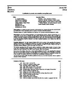
Figure 1.1: Weights in a random sample of 100 women
2.4
Figure 1.1 is a histogram of measured weight in a sample of 100 individuals. i
Would it be better to use the mean and standard deviation or the median and interquartile range to summarize this data ? The data appears to be positively skewed, so the median and inter-quartile range would provide a better summary than the mean and SD.
ii
If the mean of the data is 69.69kg with a standard deviation of 12.76kg, calculate a 95% confidence interval for the mean.
Standard Error = = ⇒ Confidence Interval = =
√ 12.76kg/ 100 1.276kg 69.69kg ± 1.96 × 1.276 (67.2kg, 72.2kg)
5
iii
3
Why is it not sensible to calculate a 95% reference range for this data ? This data is not normally distributed, so a reference range is not appropriate
Proportions
Again using our height and weight dataset of 412 individuals, 234 (56.8%) are women and 178 (43.2%) are men. If we take a number of smaller samples from this population, the proportion of women will vary, although they will tend to be scattered around 57%. Figure 1.2 represents 50 samples, each of size 40.
Fraction
.2
0 0
.25
.5 prop
.75
1
Figure 1.2: Proportion of Women in 50 samples of size 40
6
3 Proportions 3.1
What would you expect to happen if the sample sizes were bigger, say n=100 ? ................................................................................ ................................................................................ Larger samples would lead to less variation in the sample means
3.2
In a sample of 40 individuals from a larger population, 25 are women. Calculate a 95% confidence interval for the proportion of women in the population. ................................................................................
Proportion p = = ⇒ Standard Error = = = ⇒ Confidence Interval = =
25 40 0.625 s p(1 − p) n s 0.625 × 0.375 40 0.07655 0.625 ± 1.96 × 0.07655 0.475, 0.775
Note: When sample sizes are small the use of standard errors and the normal distribution does not work well for proportions. This is only really a problem if p (or (1-p)) is less than 5/n (i.e. there are less than 5 subjects in one of the groups).
3.3
From a random sample of 80 women who attend a general practice, 18 report a previous history of asthma.
7
i
Estimate the proportion of women in this population with a previous history of asthma, along with a 95% confidence interval for this proportion.
Proportion p = = ⇒ Standard Error = = ⇒ Confidence Interval = =
ii
18 80 0.225 s 0.225 × 0.775 80 0.04669 0.225 ± 1.96 × 0.04669 (0.133, 0.317)
Is the use of the normal distribution valid in this instance ? ......................................................................... Yes, since there are more than 5 subjects in each of the two groups (with and without asthma).
3.4
In a random sample of 150 Manchester adults it was found that 58 received or needed to receive treatment for defective vision. Estimate the proportion of adults in Manchester who receive or need to receive treatment for defective vision, a 95% confidence interval for this proportion.
i
ii
Proportion Proportion p =
58 150
= 0.387
95% Confidence interval
Proportion p = = ⇒ Standard Error = = ⇒ 95% Confidence Interval = =
8
58 150 0.387 s 0.387 × 0.613 150 0.03977 0.387 ± 1.96 × 0.03977 (0.309, 0.465)
4 Confidence Intervals in Stata
4
Confidence Intervals in Stata
Load the blood pressure data in its wide form into stata with the command sysuse bpwide This is fictional data concerning blood pressure before and after a particular intervention. 4.1
Use the command histogram bp_before to see if this variable is normally distributed. What do you think ? No: the data is positively skewed
4.2
Create a new variable to measure the change in blood pressure and find its mean value with the commands generate bp_diff = bp_after - bp_before summarize bp_diff What is the mean change in blood pressure ?
4.3
-5.09
Create a confidence interval for the change in blood pressure with the command ci bp_diff Does the intervention reduce blood pressure in general ? Yes, the confidence interval for the mean change in the population is (-8.1, -2.1), suggesting that there has been a reduction in blood pressure.
4.4
Look at the histogram of changes in blood pressure using the command histogram bp_diff Does this confirm your answer to the previous question ? The bulk of the histogram is to the left of 0, suggesting there has been an overall reduction in blood pressure
4.5
Create a new variable to measure whether blood pressure went up or down in a given subject using the command generate down = bp_after < bp_before Use the tabulate command to see how many subjects, and what proportion, showed a decrease in blood pressure. 73 subjects, 60.8%
4.6
Create a confidence interval for the proportion of subjects showing a decrease in blood pressure with the command ci down, binomial Does this confirm the effect of the intervention on blood pressure ? The confidence interval is (51.5%, 69.6%), suggesting that in the population more than half and possibly as many as two thirds of subjects will have a reduction in blood pressure.
9
Repeat
Sample Size 5 Sample Size 25 Sample Size 100
1
2
3
4
5
6
7
8
9
10
Mean
Standard Deviation Table 1.1: Means of random samples of different sizes
10