Practical Hierarchical Reinforcement Learning in Continuous Domains

THESIS submitted in partial fulfillment of the requirements for the degree of

MASTER OF SCIENCE IN ARTIFICIAL INTELLIGENCE

Practical Hierarchical Reinforcement Learning in Continuous Domains

Author: Sander van Dijk 1267493

14th January 2009

Supervisors: Prof. Dr. Lambert Schomaker (University of Groningen)

Drs. Tijn van der Zant (University of Groningen)

ii

Contents Abstract

v

Acknowledgements 1 Introduction 1.1 Learning . . . . . . . 1.2 RoboCup . . . . . . 1.3 3D Simulation . . . . 1.3.1 Environment 1.3.2 Agent . . . . 1.3.3 Percepts . . . 1.3.4 Actions . . . 1.4 2D Simulation . . . . 1.5 Problem Description 1.6 Organization . . . .

vii . . . . . . . . . .

. . . . . . . . . .

. . . . . . . . . .

. . . . . . . . . .

. . . . . . . . . .

. . . . . . . . . .

. . . . . . . . . .

. . . . . . . . . .

. . . . . . . . . .

. . . . . . . . . .

. . . . . . . . . .

. . . . . . . . . .

. . . . . . . . . .

. . . . . . . . . .

. . . . . . . . . .

. . . . . . . . . .

. . . . . . . . . .

. . . . . . . . . .

. . . . . . . . . .

1 1 3 4 4 5 5 7 9 10 10

2 Reinforcement Learning in Continuous Domains 2.1 Introduction . . . . . . . . . . . . . . . . . . . . . . 2.2 Methods . . . . . . . . . . . . . . . . . . . . . . . . 2.2.1 Markov Decision Processes . . . . . . . . . 2.2.2 Value Learning . . . . . . . . . . . . . . . . 2.2.3 Exploration . . . . . . . . . . . . . . . . . . 2.2.4 Reverse Experience Cache . . . . . . . . . . 2.2.5 RL in Continuous Environments . . . . . . 2.2.6 HEDGER . . . . . . . . . . . . . . . . . . . 2.3 Experiments . . . . . . . . . . . . . . . . . . . . . . 2.3.1 2D Environment . . . . . . . . . . . . . . . 2.3.2 3D Environment . . . . . . . . . . . . . . . 2.4 Results . . . . . . . . . . . . . . . . . . . . . . . . . 2.5 Discussion . . . . . . . . . . . . . . . . . . . . . . .

. . . . . . . . . . . . .

. . . . . . . . . . . . .

. . . . . . . . . . . . .

. . . . . . . . . . . . .

. . . . . . . . . . . . .

. . . . . . . . . . . . .

. . . . . . . . . . . . .

. . . . . . . . . . . . .

. . . . . . . . . . . . .

. . . . . . . . . . . . .

. . . . . . . . . . . . .

. . . . . . . . . . . . .

. . . . . . . . . . . . .

. . . . . . . . . . . . .

. . . . . . . . . . . . .

. . . . . . . . . . . . .

. . . . . . . . . . . . .

. . . . . . . . . . . . .

13 13 14 14 15 16 16 17 18 21 21 21 23 27

3 Hierarchical Reinforcement Learning 3.1 Introduction . . . . . . . . . . . . . . . . 3.2 Methods . . . . . . . . . . . . . . . . . . 3.2.1 Semi Markov Decision Problems 3.2.2 Options . . . . . . . . . . . . . . 3.2.3 Value Function . . . . . . . . . . 3.2.4 Learning an Option’s Policy . . . 3.3 Experiments . . . . . . . . . . . . . . . . 3.3.1 2D Environment . . . . . . . . . 3.3.2 3D Environment . . . . . . . . . 3.4 Results . . . . . . . . . . . . . . . . . . .

. . . . . . . . . .

. . . . . . . . . .

. . . . . . . . . .

. . . . . . . . . .

. . . . . . . . . .

. . . . . . . . . .

. . . . . . . . . .

. . . . . . . . . .

. . . . . . . . . .

. . . . . . . . . .

. . . . . . . . . .

. . . . . . . . . .

. . . . . . . . . .

. . . . . . . . . .

. . . . . . . . . .

. . . . . . . . . .

. . . . . . . . . .

. . . . . . . . . .

29 29 31 31 31 32 33 33 33 34 34

. . . . . . . . . .

. . . . . . . . . .

. . . . . . . . . .

. . . . . . . . . .

. . . . . . . . . .

. . . . . . . . . .

. . . . . . . . . .

. . . . . . . . . .

. . . . . . . . . .

. . . . . . . . . .

. . . . . . . . . .

iii

. . . . . . . . . .

. . . . . . . . . .

. . . . . . . . . .

. . . . . . . . . .

. . . . . . . . . .

. . . . . . . . . .

. . . . . . . . . .

. . . . . . . . . .

. . . . . . . . . .

. . . . . . . . . .

. . . . . . . . . .

iv

CONTENTS 3.5

Discussion . . . . . . . . . . . . . . . . . . . . . . . . . . . . . . . . . . . . . . . . .

4 Sub-Goal Discovery 4.1 Introduction . . . . . . . . . . . . . . . . . . . . . 4.2 Methods . . . . . . . . . . . . . . . . . . . . . . . 4.2.1 Multiple-Instance Learning Problem . . . 4.2.2 Diverse Density . . . . . . . . . . . . . . . 4.2.3 Sub-Goal Discovery using Diverse Density 4.2.4 Continuous Bag Labeling . . . . . . . . . 4.2.5 Continuous Concepts . . . . . . . . . . . . 4.2.6 Filtering Sub-Goals . . . . . . . . . . . . 4.3 Experiments . . . . . . . . . . . . . . . . . . . . . 4.3.1 2D Environment . . . . . . . . . . . . . . 4.3.2 3D Environment . . . . . . . . . . . . . . 4.4 Results . . . . . . . . . . . . . . . . . . . . . . . . 4.5 Discussion . . . . . . . . . . . . . . . . . . . . . .

. . . . . . . . . . . . .

. . . . . . . . . . . . .

. . . . . . . . . . . . .

. . . . . . . . . . . . .

. . . . . . . . . . . . .

. . . . . . . . . . . . .

. . . . . . . . . . . . .

. . . . . . . . . . . . .

. . . . . . . . . . . . .

. . . . . . . . . . . . .

. . . . . . . . . . . . .

. . . . . . . . . . . . .

. . . . . . . . . . . . .

. . . . . . . . . . . . .

. . . . . . . . . . . . .

. . . . . . . . . . . . .

. . . . . . . . . . . . .

. . . . . . . . . . . . .

. . . . . . . . . . . . .

39 41 41 42 42 43 43 45 46 47 50 50 52 52 56

5 Discussion

57

6 Future Work

59

A Functions A.1 Sine . . . . . . . . . . . . . . . . . . . . . . . . . . . . . . . . . . . . . . . . . . . . A.2 Distance . . . . . . . . . . . . . . . . . . . . . . . . . . . . . . . . . . . . . . . . . . A.3 Kernel Functions . . . . . . . . . . . . . . . . . . . . . . . . . . . . . . . . . . . . .

61 61 63 64

B Bayes’ Theorem

65

C Statistical Tests

67

D Nomenclature

69

E List E.1 E.2 E.3

73 73 74 75

of Symbols Greek Symbols . . . . . . . . . . . . . . . . . . . . . . . . . . . . . . . . . . . . . . Calligraphed Symbols . . . . . . . . . . . . . . . . . . . . . . . . . . . . . . . . . . Roman Symbols . . . . . . . . . . . . . . . . . . . . . . . . . . . . . . . . . . . . .

Abstract This study investigates the use of Hierarchical Reinforcement Learning (HRL) and automatic sub-goal discovery methods in continuous environments. These are inspired by the RoboCup 3D Simulation environment and supply navigation tasks with clear bottleneck situations. The goal of this research is to enhance the learning performance of agents performing these tasks. This is done by implementing existing learning algorithms, extending these to continuous environments and by introducing new methods to improve the algorithms. Firstly, the HEDGER RL algorithm is implemented and used by the agents to learn how to perform their tasks. It is shown that this learning algorithm performs very well in the selected environments. This method is then adapted to decrease computational complexity, without affecting the learning performance, to make it even more usable in real-time tasks. Next, this algorithm is extended to create a hierarchical learning system that can be used to divide the main problem in easier to solve sub-problems. This hierarchical system is based on the Options model, so only minor adjustments of the already implemented learning system are needed for this extension. Experiments clearly indicate that such a layered model greatly improves the learning speed of an agent, even at different amounts of high level knowledge about the task hierarchy supplied by the human designer. Finally, a method to automatically discover usable sub-goals is developed. This method is a thoroughly improved extension of an existing method for discrete environments. With it the agent is able to discover adequate sub-goals and to build his own behavior hierarchy. Even though this hierarchy is deduced without any extra high level knowledge introduced by the designer, it is still shown that it can increase the speed of learning a task. In any case it supplies the agent with solutions for sub-tasks that can be reused in other problems. At every step of the research experiments show that the new algorithms and adaptations of existing methods increase the performance of an agent in tasks in complex, continuous environments. The resulting system can be used to develop hierarchical behavior systems in order to speed up learning, for tasks such as robotic football, navigation and other tasks in continuous environments where the global goal can be divided into simpler sub-goals.

v

vi

ABSTRACT

Acknowledgements Even though my name is printed on the front of this dissertation, the completion of it would not have been possible without the support of others. Firstly I thank my supervisors, Prof. Dr. Lambert Schomaker and Drs. Tijn van der Zant, for giving me advice and inspiration during my research, though still giving me the opportunity to venture out into new areas of the field of Artificial Intelligence. I also am very grateful to the people who took the time to proofread my thesis and drown me in useful critique and tips, specifically Mart van de Sanden and Stefan Renkema, which helped greatly in improving the document you have in front of you. Much thanks also goes out to Martin Klomp, with who I was able to share the ordeals of producing a thesis during our many well deserved and highly productive coffee breaks. During my research I was able to gain a lot of experience, both in the field of AI as in general life, by participating in the RoboCup championships. I would like to thank the University of Groningen, its relevant faculties and the department of AI for the financial support that made it possible to attend these competitions. Eternal gratitude also goes out to the team members of the RoboCup 3D Simulation team Little Green BATS, of which I am proud to be a member, for the unforgettable times during these adventures and for their work on the award winning code base that formed a base for my research. Many thanks to them and anybody else who is part of the wonderful RoboCup experience. Last but not least I would like to thank my parents, Wybe and Olga van Dijk. Their wisdom and unconditional love and support during my educational career and any of my other choices powered me to develop myself, pursue my dreams and to handle any challenge in life.

vii

viii

ACKNOWLEDGEMENTS

Chapter 1

Introduction 1.1

Learning

Although they may have the reputation of being unreliable and flukey and people project human attributes on them, such as stubbornness, autonomy and even outright schadenfreude, computers are actually very reliable. They will do exactly what they are programmed to do, except in case of hardware failure. This property is important in high risk situations where you do not want the machine to do unforeseen things. However, in some cases a little bit of creativity on the side of the machine would not hurt. For instance, when hardware failure does occur it would be nice if the machine could adapt to it and still do its job right. More generally, in any case where the system can encounter unforeseen situations, or where the environment it has to work in is just too complex for the designer to account for every detail, a traditional preprogrammed machine will probably behave suboptimally. Here the system would benefit if it had the capability to learn. Learning is well described by Russell and Norvig [42]: The idea behind learning is that percepts should be used not only for acting, but also for improving the agent’s ability to act in the future. Learning takes place as a result of the interaction between the agent and the world, and from observation by the agent of its own decision-making processes. The term agent will be used throughout this thesis. There has been a lot of discussion about the correct definition [54], but for this thesis I will use the following simple definition, again by Russell and Norvig [42]: Definition 1 An agent is something that perceives and acts. Note that this definition includes humans, dogs and other animals, but also artificial systems such as robots. Moreover it makes no distinction between things in the real world and things in a virtual world inside a computer. What exactly entails perceiving and acting is also a huge, philosophical point of discussion in its own right, but for this thesis most common sense definitions will suffice. Traditionally learning tasks are divided into several types of problems: Supervised Learning In supervised learning an agent has to map input to the correct output (or perceptions to the correct actions) based upon directly perceivable input-output pairs. The agent receives an input and gives a prediction of the correct output. After that it directly receives the correct output. Based on the difference between the predicted and the correct output he can learn to perform better in the future by improving his prediction process. A stockbroker for instance predicts the worth of a stock for the next day based upon the information he has about recent stock development. The next day he perceives the actual worth and uses this to improve his prediction method. 1

2

CHAPTER 1. INTRODUCTION

Unsupervised Learning When there is no hint at all about what the correct output is or which the right actions are, learning is said to be unsupervised. In these cases the problem consists of finding relationships in and ordering unlabeled data. An example could be ordering letters on a scrabble rack. There is no ’right’ or ’wrong’ way to do this and it can be done based on letter worth, alphabetic order or the number of people you know with the letters in their name. Reinforcement Learning On the scale of amount of feedback, between supervised and unsupervised learning we find Reinforcement Learning (RL). Agents in a RL problem receive some feedback on the success of their actions, but not in as much detail as in supervised tasks. The agent for instance is told his output or actions are good, mediocre or bad, but has to find out what exactly the best option is on his own. Also, often he only gets a delayed reward, i.e. he only gets feedback after performing a series of actions but is not told directly which of those actions was most responsible for this reward. Think of a chess player who only gets the feedback ’you won’ or ’you lost’ at the end of a game and has to figure out which intermittent board states are valuable and which of his moves were mostly responsible for the outcome of the game. Biological agents, such as us, perform very well in all three of these learning problems. Throughout our lifes we learn new abilities, improve old ones and when not to use some of our abilities. Even much simpler animals like mice have a great ability to adapt to new situations. Artificial agents on the other hand are far behind on their biological examples. In many experiments it is not unusual for an agent to require thousands, or even millions of tries before he has learnt a useful solution or a certain behavior. Getting machines to learn on their own is one of the major tasks in the field of Artificial Intelligence (AI). In the early years of this research field the focus was on game-like problems, such as tic-tac-toe, checkers or, most importantly, chess. These problems usually have some of the following properties in common [42]: Accessible An agent has access to the full state of the environment. A chess player can see where all the pieces are on the board. Static The world does not change while the agent is thinking about his next move. Discrete There is a limited amount of distinct, clearly defined possible inputs and outputs, or percepts and actions, available to the agent. There is only a limited amount of possible combinations of piece positions on a chessboard and the possible moves are restricted by the type and position of these pieces. In other words: it is possible to give each and every state and action a distinct, limited number. The overall consensus was that the ability to handle these kinds of problems sets us apart from other animals. Unlike, say, chimpanzees we are able to perform the discrete, symbolic, logical reasoning needed to play a game such as chess, so this was seen as real intelligence. If an artificial system could solve these problems too, we would have achieved AI. Thanks to research on these problems a lot of innovative ideas and solutions to machine game playing came about, finally resulting in the victory of a chess playing computer over the human world champion. However, this victory was due to the massive amount of computing power available to the artificial player, not so much thanks to what most people would think of as intelligent algorithms. Even though the human player said the play of the computer seemed intelligent, creative and insightful, this was only the result of being able to process millions of possible future moves in a matter of seconds. At this time, AI researchers also found out that the traditional symbolic methods used to solve these kinds of problems do not work well when trying to control a robot in a real world environment. The real world is infinitely more complex and ever changing, exponentially increasing the processing power needed to handle it on a symbolic level. Moreover, the real world does not easily and unambiguously translate into nicely defined, discrete symbols. Attempts to create

1.2. ROBOCUP

3

intelligent robots that act upon the real world resulted into big piles of electronics, moving at less than a snail like pace, getting totally confused when the world changed while they were contemplating what to do next. In the 1980’s the realization that things should change kicked in. The most expensive robots were terribly outperformed by simple animals with much less computing power, such as fish and ants. The focus shifted towards more realistic every day worlds. These environments have much more demanding properties, as opposed to those listed earlier for game-like problems [42]: Inaccessible Not all information about the environment is readily available to an agent. A football player cannot see what is going on behind him, he has to infer this from his memory and from ambiguous percepts such as shouting by his teammates. Dynamic The world changes while the agent thinks. The other football players do not stand still and wait while an agent is contemplating to pass the ball to a team member. Continuous There is an infinite number of possible states and sometimes also an infinite number of possible actions. You cannot number the positions of a football player in the field. Between each two positions is another position, between that one and the other two arr two others, et cetera ad infinitum. Early breakthroughs showed that using much simpler subsymbolic solutions is much more efficient. Simple direct connections between sensors and actuators already result in complex, fast and adaptive behavior [9, 10]. This shift of focus also meant that the field needed a new standard problem to replace the old chessboard.

1.2

RoboCup

This new problem became RoboCup, the Robot World Cup Initiative. One of the important reasons why the chess problem pushed AI research forward was the element of competition. In 1997 the RoboCup project was started to introduce this same element into the new generation of smart machines: RoboCupTM is an international joint project to promote AI, robotics, and related field. It is an attempt to foster AI and intelligent robotics research by providing a standard problem where a wide range of technologies can be integrated and examined. RoboCup chose to use the football game as a central topic of research, aiming at innovations to be applied for socially significant problems and industries. The ultimate goal of the RoboCup project is: By 2050, develop a team of fully autonomous humanoid robots that can win against the human world champion team in football. In order for a robot team to actually perform a football game, various technologies must be incorporated including: design principles of autonomous agents, multi-agent collaboration, strategy acquisition, real-time reasoning, robotics, and sensor-fusion. RoboCup is a task for a team of multiple fast-moving robots under a dynamic environment. RoboCup also offers a software platform for research on the software aspects of RoboCup. One of the major application of RoboCup technologies is a search and rescue in large scale disaster. RoboCup initiated the RoboCupRescue project to specifically promote research in socially significant issues. [2] The RoboCup project is divided into several leagues, each focusing on different parts of the overall problem. Here I will describe some of them. Middle Size League The Middle Size League (MSL) uses fast, wheeled robots that are about 3 feet high and is usually the most exciting and popular league to watch. These robots play in a field of 18x12 meters, the largest field of all real world leagues. The main challenges in this league are fast and reliable ball handling, fast paced strategies and machine vision in real world lighting conditions.

4

CHAPTER 1. INTRODUCTION

Humanoid Leagues At the moment there are 3 Humanoid Leagues: Kid Size (KHL) and Teen Size (THL), with robot sizes about 60cm and 120cm respectively, and the Standard Platform League (SPL). Whereas the teams of the first two leagues construct their own robots, all teams in the SPL use the same type of robot. Therefor the first puts more weight on the engineering aspect while in the second the actual intelligence and strategies used determine a team’s success. Simulation Leagues As discussed earlier, the whole idea behind RoboCup is to push the fields of AI and Robotics into the real world. However, already at the beginning of the effort the organizers understood the importance of simulation [25]. Ideas can be tested in software simulations before applying them to the real world leagues. This way teams do not have to risk the usually very pricey real robots to test new ideas. Virtual robots do not break when you for instance try hundreds of experimental walking gaits on them. Also in simulations you can already work on higher level solutions before the real world leagues are ready for them. You can for instance work on a kicking strategy based on a stereoscopic vision system while the real robots still only use one camera and transfer the obtained knowledge to the other leagues when they have advanced far enough. Finally, the simulation leagues give a low cost entry into the RoboCup world for teams with low budgets, making sure talent is not wasted due to financial issues. The simulation leagues started with the 2D Simulation League (2DSL). In this league virtual football players, abstract discs, play in a 2-dimensional field. It is the only league with full 11 versus 11 games and the main focus is on high level team play. Games in the 2DSL are fast paced with a lot of cooperation and coordination. In 2003 the 3D Simulation League (3DSL) was introduced. Here simulations are run in a full 3-dimensional environment with natural Newtonian physics. In the first few years the agents in the 3DSL were a simple adaptation from the 2D agents: simple spheres that could move omnidirectional and ’kick’ the ball in any direction. However, in 2006 and 2007 a great effort was made to replace these spheres by full fledged humanoid robot models. This meant the teams had to shift focus from high level strategies to low level body control. Nevertheless this was a great step forward in terms of realism and the community is on its way to return to the main goal of the simulation leagues: to research high level behavior which is not yet possible or feasible on real robots. In 2008 the league used a virtual robot modeled after the Nao robot that is used in the SPL. The RoboCup championship has grown a lot over the years and is now one of the largest events in the fields of AI and Robotics in the world. Every year hundreds of teams participate, spread over more than a dozen leagues, attracting thousands of interested visitor. The RoboCup problem receives a lot of attention from the scientific world and is considered an important and valid field of research. It provides a good testbed for Reinforcement Learning, the base framework of this thesis. RL has been researched and used to train many aspects of the robots used, such as gaits for both biped as quadruped robots, standing up, team strategy, et cetera [4, 26, 41, 48, 49]. Due to the realistic nature, large amount of scientific background and ease of measuring performance through competition, the RoboCup problem is a natural choice as a testbed for new learning methods. In this thesis I will specifically use the 3D Simulation framework, as it offers a realistic, complex environment and does not suffer from hardware related problems like wear and tear when performing large amounts of test runs. Section 1.3 will describe the 3D Simulation framework in more detail and how I will use it as an experimental environment to test solutions.

1.3 1.3.1

3D Simulation Environment

The RoboCup 3D Simulation League uses a simulator program, called the server, which uses the Open Dynamics Library (ODE) to simulate a football game [38]. The dynamics of the simulation

1.3. 3D SIMULATION

5

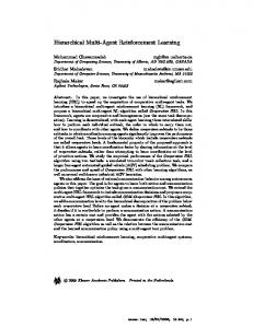
Figure 1.1: The 3D Football simulation field. The field is 12x8 meters in size and contains two colored goals and the ball. Two humanoid agents are placed in the field. At the top of the simulator window the scores, game state and game time are shown.

include realistic, Newtonian physics such as gravity, friction and collisions. The environment that is simulated consists of a simple football field, modeled after the fields used in the real world leagues (see Figure 1.1). The field contains two goals and a ball. The simulation has a built in referee that can enforce football rules, including goals and outs, half times and player and ball positions. For instance, when the ball leaves of the field, the opponents of the team touch the ball last get a free kick at the field line. Players of the other team cannot get close to the ball until the kick in is taken.

1.3.2

Agent

The agents used in the 3D Simulations are models of humanoid robots. It is based on the Nao robot and has realistic sizes, weights, et cetera. Figure 1.3 shows the simulated agent in the football field along with his joints that make up its Degrees Of Freedom (DOFs). The agents are controlled by separate, standalone programs, or clients, that connect to the server through a TCP/IP connection. This allows the server and clients to be run on different computers, distributing the computational load. Information between the server and the clients is done through text based, LISP-like structures called S-expressions, such as those shown in figure 1.2.

1.3.3

Percepts

The virtual robot has a number of ways to get information about his environment. Just like the real Nao robot he has several sensors through which he receives percepts about his body and objects in the field:

6

CHAPTER 1. INTRODUCTION

( (time (now 131.15)) (GS (t 0.00) (pm BeforeKickOff)) (GYR (n torso) (rt -43.86 -15.00 39.54)) (See (G1L (pol 2.93 -135.07 -10.50)) (G2L (pol 4.20 -125.57 -8.63)) (G2R (pol 11.33 -42.24 30.93)) (G1R (pol 10.92 -34.42 32.82)) (F1L (pol 1.62 124.25 -37.28)) (F2L (pol 7.38 -113.48 -11.96)) (F1R (pol 10.65 -13.23 30.94)) (F2R (pol 12.85 -55.43 22.53)) (B (pol 5.65 -55.57 20.83))) (HJ (n hj1) (ax -0.00)) (HJ (n hj2) (ax 0.00)) (HJ (n raj1) (ax -90.00)) (HJ (n raj2) (ax -0.00)) (HJ (n raj3) (ax -0.00)) (HJ (n raj4) (ax -0.00)) (HJ (n laj1) (ax -90.00)) (HJ (n laj2) (ax -0.00)) (HJ (n laj3) (ax -0.00)) (HJ (n laj4) (ax -0.00)) (HJ (n rlj1) (ax -0.00)) (HJ (n rlj2) (ax -0.00)) (HJ (n rlj3) (ax 64.53)) (HJ (n rlj4) (ax -38.73)) (HJ (n rlj5) (ax 6.90)) (HJ (n rlj6) (ax -0.00)) (HJ (n llj1) (ax -0.00)) (HJ (n llj2) (ax 0.00)) (HJ (n llj3) (ax 56.24)) (HJ (n llj4) (ax -61.27)) (HJ (n llj5) (ax 33.25)) (HJ (n llj6) (ax -0.00)) (FRP (n lf) (c 0.04 0.08 -0.02) (f -14.74 -6.94 -1.85)) (FRP (n rf) (c 0.03 0.08 -0.02) (f -15.73 -27.71 111.58)) ) Figure 1.2: Example of information sent to an agent by the simulation server. The data contains game state information, including the current time and play mode, as well as sensory data. This sensory data consists of the angular velocity measured by a gyroscopic sensor (GYR), vision information of objects in the field such as goals (G1L etc.), corner flags (F1L etc.) and the ball, joint angle values (HJ) and foot pressure measured by the Force Resistance Perceptors (FRP).

(a) Front

(b) Side

Figure 1.3: RoboCup 3D Simulation humanoid agent. 1.3a shows the agent’s front, 1.3b his side. The agent’s leg and head joints are also depicted.

7

1.3. 3D SIMULATION Number 1 2 3 4 5 6 7 8 9 10 11 12 13 14 15 16 17 18 19 20 21 22

Name HEAD1 HEAD2 LLEG1 LLEG2 LLEG3 LLEG4 LLEG5 LLEG6 RLEG1 RLEG2 RLEG3 RLEG4 RLEG5 RLEG6 LARM1 LARM2 LARM3 LARM4 RARM1 RARM2 RARM3 RARM4

Description Neck, z-axis Neck, x-axis Left hip, xz-axis Left hip, x-axis Left hip, y-axis Left knee, x-axis Left ankle, x-axis Left ankle, y-axis Right hip, xz-axis Right hip, x-axis Right hip, y-axis Right knee, x-axis Right ankle, x-axis Right ankle, y-axis Left shoulder, x-axis Left shoulder, y-axis Left shoulder, z-axis Left elbow, x-axis Right shoulder, x-axis Right shoulder, y-axis Right shoulder, z-axis Right elbow, x-axis

Range (deg) (-120, 120) (-45, 45) (-90, 1) (-25, 100) (-25, 45) (-130, 1) (-45, 75) (-45, 25) (-90, 1) (-25, 100) (-45, 25) (-130, 1) (-45, 75) (-25, 45) (-120, 120) (-1, 95) (-120, 120) (-90, 1) (-120, 120) (-95, 1) (-120, 120) (-1, 90)

Table 1.1: Description of the joints of the 3D simulation robot. For placement of most joints see figure 1.3.

Joint Sensors Each joint of the robot has a sensor connected to it that measures the current angle of the joint. Gyroscopic Sensor A gyroscopic sensor in the robot’s torso gives the agent a measure of his angular velocity around the x, y and z axis. Force Resistance Perceptor On the sole of each foot the robot has a Force Resistance Perceptor (FRP), which measures the total force vector on it and gives a position on the foot where the force acts upon. Vision The robot has a camera in his head that gives him the ability to perceive other objects in the world. It is assumed that the robot has a built in state of the art vision processor that can extract details about these objects. This processor gives information about the relative position to the agent of the ball, goal posts, field corners and of other players. At the moment the agent can see everything, 360 degrees around him, so called omnivision, without any noise in the information. To make the simulation more realistic, the official RoboCup simulation will move to a vision system with a restricted viewing angle and will add noise to the output. Hearing Because direct communication between the clients through for instance TCP/IP connections is not allowed, the robots are given hearing perceptors and complementing speech effectors. Using this the agents can communicate by shouting short messages to each other.

1.3.4

Actions

An agent is able to affect the environment he is in through effectors. He can use these to make changes in the world. The 3D Simulation agent has access to several effectors.

8

CHAPTER 1. INTRODUCTION

Joint motors Each joint has a motor connected to it. The agent can set desired rotational velocities for each motor, which the simulator will try to achieve as fast as possible, limited by a maximum possible amount of torque that the motor can generate. These motors are the most important effectors for the agent and he should control them all harmoniously to create useful motion. Speech As mentioned in the previous section, each agent is able to shout short messages. These can be heard by other agents up to a certain distance. Agents can use this ability to coordinate their actions or inform each other about the environment when the restricted vision system is used. Using the joint motors agents can generate wide ranges of high level actions, for instance waving, kicking and walking. The latter is the most important skill for this thesis, since the football environment is large and the agent has to move around a lot to play successfully. To humans walking seems very easy. We perform this task daily, without consciously thinking about it. But actually walking is a very complex behavior, created by controlling and intimately coordinating the movement of muscles throughout our bodies, mediated by information of a huge amount of perceptors. We not only use our legs, but also our hips, back and arms to stabilize, with input from for instance pressure perceptors in our feet, joint angle perceptors and the otolithic organ in our ears. To develop such a movement method for humanoid, bipedal robots is a whole research field in its own right. Many researchers try many different methods to develop stable, fast walking gaits for humanoid robots [22, 46, 55]. Such a robot is usually a much simpler system than a human body, making whole body control easier. However, they still usually have several dozens of DOFs and perceptors, making the entire state and action space huge. Though, ironically, most humanoid robots could use even more DOFs to achieve human-like behavior. For instance, most robots cannot turn their torso relative to their hip, which is a very important part of human walking. In this thesis I will use a simple open loop walking gait. This means that the robot does not use any feedback from its sensors, such as foot pressure or angular velocity, to stabilize itself. Since the surface is perfectly flat and the agent will not turn or change directions rapidly, such an open loop method is sufficient for these experiments. The gait used is one of the walking gaits of the Little Green BATS RoboCup 3D simulation team developed for and used during the 2007 and 2008 RoboCup World Championships [1]. It is based upon the observation that a walking gait is cyclic, i.e. after a swing of the left and then the right leg the movement starts over again. To achieve this oscillating kind of motion, the most basic oscillating function is used to control the agent’s joints. Each joint is controlled separately by a sinusoidal pattern generator: αdi (t) =

N X j=1

Aij sin(

t 2π + ϕij ) + Cij . Tij

(1.1)

Here αdi (t) is the desired angle for joint i at time t, Aij is the amplitude of the swing of the joint, T is the period of a single swing, ϕij is the phase offset of the oscillation and C is a constant offset angle around which the joint will oscillate. By increasing N the motion can be made as complex as desired, however for the gait used here N ≤ 2 is sufficient to create reliable directed movement. Different parameters are used to create gaits for walking forwards, backwards, left and right. To create these, first an in-place stepping pattern is created using the parameters given in table 1.2. This pattern causes up and down movement of the feet. By adding joint movement that is out of phase with this stepping pattern we can add horizontal movement of the feet, making the robot move. The parameters for this overlayed movement are given in table 1.3. The RoboCup 3D Simulation robot is controlled by setting the angular velocity of the joint motors. To determine these velocities based on the outcome of equation 1.1 a simple proportional controller is used: ωi (t) = γ(αdi (t) − αi (t)), (1.2)

9

1.4. 2D SIMULATION Joint 2 4 5

A(deg) 4 -8 4

T (s) 0.5 0.5 0.5

ϕ 0 0 0

C(deg) 60 -50 18

Table 1.2: Parameters for the sinusoidal joint control using equation 1.1 to create an in-place stepping pattern, where A is the amplitude of the joint swing, T the period, ϕ the phase and C a constant offset. Joint descriptions are given in table 1.1 and figure 1.3. For the right leg the same parameters are used, but with a phase offset of π.

Joint 2 5

A(deg) -4 -4

T (s) 0.5 0.5

ϕ 1 2π 1 2π

C(deg) 0 0

Joint 2 5

(a) Forward

Joint 3 6

A(deg) -4 4

T (s) 0.5 0.5 (c) Left

A(deg) 4 4

T (s) 0.5 0.5

ϕ 1 2π 1 2π

C(deg) 0 0

ϕ 1 2π 1 2π

C(deg) 0 0

(b) Backward

ϕ 1 2π 1 2π

C(deg) 0 0

Joint 3 6

A(deg) 4 -4

T (s) 0.5 0.5

(d) Right

Table 1.3: Parameters for the sinusoidal joint control using equation 1.1 to create directed walking patterns, where A is the amplitude of the joint swing, T the amplitude, ϕ the phase and C a constant offset. The sinusoidal functions using these parameters are added to those of the stepping pattern of table 1.2. Joint descriptions are given in table 1.1 and figure 1.3. For the right leg the same parameters are used, but with a phase offset of π.

where ωi (t) is the angular velocity of joint i at time t, γ = 0.1 is a gain parameter and αi (t) is the joint angle of joint i at time t.

1.4

2D Simulation

As mentioned earlier, RL may need many runs before the system converges to a solution. Because the RoboCup 3D simulation runs in real time, this can take many days for complex tasks. So to speed up testing I will also use a simpler continuous environment. For this I have developed a 2D continuous simulation environment. The world consists of a 2 dimensional space in which obstacles can be placed to restrict an agent’s movement. There are no physical effects such as drag or gravity, making the environment very simplistic. Therefor, this environment will only be used as a preliminary ’proof of concept’ framework. Final usability and performance will be tested in the 3D simulation environment. The 2D environment is similar to those used in many earlier RL research. However, in most of this earlier research the environment is discrete. The 2D environment used in this thesis on the other hand is continuous. Obstacles can in theory have every possible shape instead of being built up by discrete blocks. The agent is a dimensionless point in the environment with a continuous, 2D position. His action space consists of four moves: up, down, left, right. When the agent performs one of these actions he is moved 5 meters into the selected direction. When an obstacle is in the way, the action fails and the agent remains at the same position. The percepts of the agent only consist of his own x,y-position within the environment.

10

CHAPTER 1. INTRODUCTION

1.5

Problem Description

In this thesis I will develop, implement and improve learning methods for artificial agents. Specifically, these agents deal with Reinforcement Learning problems in complex, continuous, real time environments. As mentioned above, one of the largest problems is that learning in this kind of environment can be very slow. Experiments where it takes thousands, even millions of runs to find a good solution are not at all unfamiliar in these settings. Therefor in this thesis I will mainly research methods that are intended to speed up learning of tasks in these environments, focusing on the following questions: 1. How can traditional RL algorithms be extended to reduce the number of trials an agent needs to perform to learn how to perform a task? 2. How can the computational processing complexity of these algorithms be minimized? By answering the first question, an agent will be able to learn more efficiently from initial attempts at performing a task. A football playing agent learning to shoot the ball at a goal for instance may need less kicking trials before becoming a prime attacker. By keeping the second question in mind, it is ensured that a learning method can be run on-line, in real time as the agent is acting in the environment. For agents learning in a simulated environment that can run faster than real time, this means the run time per trial, and thus the total learning time, is reduced. However, agents acting in a fixed time environment with limited processing power also benefit from the fact that less computational intensive learning methods allow for spare computational power to perform other tasks in parallel. So to test the performance of learning methods two measures will be used: 1. Number of trials performed before sufficiently learning a task. 2. Computation time needed by the method per trial. The usage of the term ‘sufficiently’ seems to make the first measure subjective, however it will be shown that it can be measured objectively when describing the experiments in the next chapters.

1.6

Organization

The rest of this thesis will be concerned with answering the questions put forward in the previous section. This will be done in three stages, each presented in one of the next three chapters. Firstly, in chapter 2 I will give a formal introduction to RL, implement and test a RL algorithm for agents acting in the 2D and 3D environments described earlier and introduce an adaptation to the algorithm to make it perform better based on the performance measures of the previous section. Secondly, I will extend this RL algorithm to a hierarchical method in chapter 3 to accommodate for temporally extended actions, sub-goals and sub-tasks. The performance of this system is tested against that of the simpler algorithm of chapter 2, using different amount of initial knowledge about the action hierarchy introduced by a designer. Finally, in chapter 4 I will describe a method for the agent to build up an action hierarchy automatically, introduce several novel adaptations of this method to make it more usable generally, and specifically in the continuous environments used in this thesis and again test its performance. Note that each chapter presents a separate, independent piece of research. Therefor each chapter is organized to have an introduction, a section formally describing the methods that are used, a description of the experiments done to test the methods of that chapter and a presentation and a discussion of the results obtained with these experiments. In chapter 5 all results of these three chapters are gathered and discussed in a global setting. The final chapter, chapter 6, will give pointers to future work. To help the reader, several appendices are added to this thesis. Appendices A, B and C give a more thorough introduction into some of the basic concepts that are used in this thesis. Next to

1.6. ORGANIZATION

11

that, throughout this thesis technical terms and abbreviations are introduced and used. To help the reader remember the definition of these, a short description of all emphasized terms is given in appendix D. Finally, appendix E lists and describes all variables used in the equations, pieces of pseudo code and text of this thesis.

12

CHAPTER 1. INTRODUCTION

Chapter 2

Reinforcement Learning in Continuous Domains 2.1

Introduction

The main goal of this thesis is to allow agents to discover sub-goals in unknown environments. However, before an agent can do this reliably, he needs a way to learn how to act in these environments. He has to find out how to achieve his goals, before he can decide upon adequate sub-goals. To direct the agent’s learning, he will be presented rewards when he manages to achieve a goal. The task of using rewards to learn a successful agent function is called Reinforcement Learning (RL) [42]. The problem to solve in this task is to find out which actions resulted in these rewards. A chess player may play a game perfectly, except for one bad move half way which causes him to lose in the end. After the game he has to figure out which move was the bad one. Humans, dogs and other animals are very good at solving this kind of problems and over the years a lot of progress is made in the field of artificial intelligence on developing RL methods for training controllers of artificial agents. One of the first examples of RL is Donald Michie’s Matchbox Educable Noughts And Crosses Engine (MENACE) ’machine’ [34] which learns the best strategy for the game of tic-tac-toe. This machine consisted of approximately 300 matchboxes, one for each possible board state, filled with 9 colors of marbles, one for each possible move in that state. At every move Michie selected the correct matchbox and took a random marble out of it, representing the move that the machine makes, after which the marble is put on top of the matchbox. If the machine wins, the marbles of the last game are put back into their boxes, along with 2 extra marbles of the same color. If he loses, the marbles are removed. This way the probability of performing moves that were successful in earlier games rises, resulting in an improved strategy. More recently, RL is used to develop controllers for highly non-linear systems. For instance, Morimota and Doya [37] present a RL system that learns how a simplified humanoid robot can stand up from lying on the floor. They do this using a double layered architecture to split the difficult problem into several parts. The first layer learns what body positions are adequate subgoals, the second learns how to achieve these positions. However, though these examples are very interesting and impressive, they still do not compare to their biological counterparts. They still need a massive amount of trials to learn tasks compared to biological agents. For instance, the 3 segment swimming agents of Coulom [13] needed over 2 million trials to learn good swimming policies. Also, trained controllers are not often reusable in different or even similar tasks. In this thesis learning algorithms will be introduced, implemented and tested that can help to bring artificial learning at the same level of biological learning. This chapter focuses on creating a basic RL mainframe for complex environments. Section 2.2 will introduce the theoretical background of RL and describes the HEDGER RL algorithm that is used in this thesis. After that, section 2.3 will describe the experiments used to 13

14

CHAPTER 2. REINFORCEMENT LEARNING IN CONTINUOUS DOMAINS

test this method in the environments described in chapter 1. The results of these experiments are presented and discussed in sections 2.4 and 2.5.

2.2 2.2.1

Methods Markov Decision Processes

Markov Decision Processes (MDPs) are the standard reinforcement learning frameworks in which a learning agent interacts with an environment at a discrete time scale [29]. This framework is used to describe the dynamics and processes of the environments and agents used in this thesis. An MDP consists of the four-tuple < S, A, P, R >, where S is the state space, A is the action space, P is the state-transition probability distribution function and R is the one-step expected reward. Sometimes not all actions can be executed in each state, therefore we define for each state s a set As ⊆ A of actions that are available in that state. The rest of this section is a formal description of MDPs as given by Sutton and Barto [50]. The probability distribution function P and one-step reward R are defined as follows: a Pss ′ Rass′

= P (st+1 = s′ |st = s, at = a); = E{rt+1 |st = s, at = a, st+1 = s′ },

(2.1) (2.2)

for all s, s′ ∈ S and a ∈ As , where st is the state of the world at time t, at is the action performed by the agent at time t and E{rt } is the expected reward received in state st . These two sets of quantities together constitute the one-step model of the environment. They show that the next state of the world only depends on the previous state, which is the so called Markov-property that gives MDPs their name. An MDP describes the dynamics of an agent interacting with its environment. The agent has to learn a mapping from states to probabilities of taking each available action π : S × A → [0, 1], where π(s, a) = P (at = a|st = s), called a Markov-policy. A policy determines together with the MDP a probability distribution over sequences of state/action pairs. Such a sequence is called a trajectory. The usability of a policy depends on the total reward an agent will gather when he follows this policy. This reward is defined as: Rt = rt+1 + γrt+2 + γ 2 rt+3 + ... =

1 X

γ k rt+k+1 ,

(2.3)

k=0

where γ is a parameter, 0 ≤ γ ≤ 1, called the discount rate, which determines how highly an agent values future rewards. Rt is called the total discounted future reward. Given this quantity, we can define the value of following a policy π from a state s (or: the value of being in state s when committed to following policy π) as the expected total discounted future reward an agent will receive: V π (s) = =

Eπ {Rt |st = s, π} ( 1 ) X k γ rt+k+1 |st = s, π Eπ k=0

= =

Eπ {rt+1 + γV π (st+1 )|st = s} X X a a π ′ π(s, a) Pss (s )] . ′ [Rss′ + γV a∈A

(2.4)

s′ ∈S

V π is called the state-value function for π. The last form of equation 2.4, which shows that the value of a state depends on an immediate reward and the discounted value of the next state, is called a Bellman equation, named after its discoverer Richard Bellman. When a policy has an

15

2.2. METHODS

expected reward higher than or equal to all other policies in all possible states it is called an optimal policy, denoted by π ∗ . An optimal policy selects the action that brings the agent to the state with the highest value, from each initial state, and maximizes the value function: V ∗ (s) = = =

max V π (s) π

max E {rt+1 + γV ∗ (st+1 )|st = s, at = a} a∈A X a a ∗ ′ max Pss ′ [Rss′ + γV (s )] . a∈A

(2.5)

s′ inS

From equation 2.5 it follows that the optimal policy selects the best action by predicting the resulting state s′ of the available actions and comparing the values of these states. This means that the agent following this policy needs to have access to the state-transition model P. In most tasks, including those of interest of this thesis, this information is not readily available and an agent has to do exhaustive exploration of the environment to estimate the transition model. To overcome this, the agent can use the action-value function Qπ (s, a) instead: Qπ (s, a) = =

Eπ {Rt |st = s, at = a} ( 1 ) X k Eπ γ rt+k+1 |st = s, at = a k=0

=

X

"

a Rass′ + γ Pss ′

s′ ∈S

X

#

π(s′ , a′ )Qπ (s′ , a′ ) .

a′

(2.6)

An optimal policy also maximizes the action-value function, resulting in the optimal actionvalue function: Q∗ (s, a) = max Qπ (s, a) π h i X a a ∗ ′ ′ = Pss ′ Rss′ + γ max Q (s , a ) . ′ a

s′ inS

2.2.2

(2.7)

Value Learning

Given the MDP framework, the problem for an agent is to determine the optimal policy π ∗ to follow. If he bases his policy on a value function, e.g.: X at = arg max Psat s′ (Rast s′ + γV (s′ )), (2.8) a∈Ast

s′ inS

or at = arg max Q(st , a),

(2.9)

a∈Ast

the problem reduces to learning the optimal value function. Many different RL methods have been developed to solve this problem, for an overview see [24] and [50]. For this thesis I will focus on and use one of the most popular methods called Temporal Difference (TD) learning. This method updates the value function based on the agent’s experience and is proven to converge to the correct solution [50]. TD works by determining a target value of a state or a state action pair, based upon experience gained after performing a single action. The current value estimate is then moved towards this target: V (st ) ← V (st ) + α [rt+1 + γV (st+1 ) − V (s)] , (2.10)

16

CHAPTER 2. REINFORCEMENT LEARNING IN CONTINUOUS DOMAINS

where 0 ≤ α ≤ 1 is the learning rate. To learn quickly this value should be set high initially, after which it should decrease slowly towards 0 to ensure convergence. In this thesis however I will use fixed learning rates for simplicity. When instead of considering transitions from state to state we look at transitions between state-action pairs, the same sort of update rule is possible for Q-values: Q(st , at ) ← Q(st , at ) + α [rt+1 + γQ(st+1 , at+1 ) − Q(st , at )] .

(2.11)

Note that this update rule is highly dependant on the current policy being followed, a so-called on-policy method, by using the value of the action chosen by that policy in the next state (at+1 ). This action however may not at all be the optimal action to perform. In this case the agent does not learn the optimal value function, needed to determine the optimal policy. An off-policy method is independent from the actual policy being followed. An important off-policy method is Q-Learning [52] which uses a different update rule: "

Q(st , at ) ← Q(st , at ) + α rt+1 + γ

max

a′ inAst+1

′

#

Q(st+1 , a ) − Q(st , at ) .

(2.12)

Using this rule the learned state-action value function directly approximates Q∗ (s, a). This results in a dramatic increase of learning speed. In this thesis I will use this method as the base for the RL algorithms used by the agents to learn their policies.

2.2.3

Exploration

The previous section gives a method to learn a policy based on experience. However, an agent using this method will stick to the first successful strategy it encounters. This might result in an agent continuously taking a long detour to reach his goal. So an agent should do some exploration to try to find better ways to perform his task. There are two main methods to promote this exploration. Firstly, before the first training run Q-values could be initialized with a value qinit > 0. If this value is set high enough, any update will likely decrease the value estimate of encountered state-action pairs. This way, next time the agent will be in a familiar state, the value estimate of yet untried actions will be higher than the estimates of previously taken actions. This causes exploration especially in the initial stages of learning, until the Q-value estimates have moved towards their real values sufficiently. The second method ensures exploration throughout the whole learning process. Instead of always taking the currently thought to be best action, the agent sometimes, with a small probability called the exploration rate ǫ, performs a random action. This action is chosen uniformly from all currently available actions As . This kind of policy is called an ǫ-greedy policy. This type of exploration ensures that eventually all actions are chosen an infinitive amount of times, which is one requirement for the guarantee that the Q-value estimates converge to Q∗ .

2.2.4

Reverse Experience Cache

When using update rule 2.12 on each experience as it is acquired by the agent, the information of this experience is only backed up one step. When the agent receives a reward, it is only incorporated into the value of the previous state. Smart introduces a way to increase the effect of important experiences [45]. To make sure such an experience has effect on the value of all states in a whole trajectory, experiences are stored on a stack. When a non-zero reward is encountered, this stack is then traversed, presenting the experience to the learning system in reverse order. This greatly speeds up learning correct value functions, by propagating the reward back through the whole trajectory.

17

2.2. METHODS

2.2.5

RL in Continuous Environments

The RL methods discussed in the previous section have been mainly developed in the context of discrete environments. In these worlds the state-action value function Q(s, a) can be implemented by a look-up table. The size of this table however increases exponentially with the number of dimensions of the state and action spaces. In complex worlds this size can quickly become intractable. This curse of dimensionality becomes even worse in the continuous environments used in this thesis. Every continuous dimension can be divided into an infinite amount of values, so using a table to store all state or state-action values is already impossible with even the lowest amount of dimensions. One way out is to discretize the space. A grid is positioned over the space and all values within the same cell of this grid are aggregated into a single cell of the state-action value look-up table. However, this makes it impossible to differentiate between states within the same cell and thus to handle situations where the optimal actions to perform in these states differ. Also, it is not possible to have smoothly changing behavior. For all states in a grid cell the same action is chosen, resulting in stepwise change of behavior when moving from one cell to another. Finer grids help to some degree to overcome these problems, but increase the curse of dimensionality again, so there is a trade-off to be made. Some methods have been proposed to make this trade-off easier. Variable resolution TD learning [36] for instance uses a coarse grid with large cells by default, but makes it finer in areas where higher precision seems to be needed to be able to learn good policies. Another way is offered by Cerebral Model Arithmetic Controllers (CMACs) [35]. This method overlays several coarse grids on the input space, each shifted with respect to the others. The system then learns the values for each cell of each grid. To calculate the final value at a certain point, a weighted average is taken of the values of the cells of each grid this point is in. This results in a finer partitioning of the space with a relatively small increase of parameters. An entirely other way of dealing with continuous domains is by abandoning the grid based approach completely and use a representation of the value function that does not rely on discretization. A system is used with a fixed amount of parameters that can estimate the output, e.g. a Q-value, given the input, e.g. state-action pairs. A learning algorithm then is used to tune the parameters of this system to improve the estimations. A lot of research has been done in the field of Machine Learning on this subject of so called function approximation. One of the most widely used class of function approximation methods is that based on gradient descent [50]. In these methods Vt (s) is a smooth differential function with a fixed number of real valued parameters ~ θt = (θt,1 , θt,2 , ..., θt,n )T . These parameters are updated at time t with a new π sample st → V (st ) by adjusting them a small amount into the direction that would most reduce the error of the prediction Vt (st ): ~ = θ~t + α(V π (st ) − Vt (st ))∇~ Vt (st ), θt+1 θt

(2.13)

~t ) ~t ) T ~t ) ∂f (θ ∂f (θ (θ where ∇θ~t f (~ θt ) denotes the vector of partial derivatives (gradient ) ( ∂f ∂θt,1 , ∂θt,2 , ..., ∂θt,n ) . Gradient descent methods get their name from the fact that the change of ~θt is proportional to the negative gradient of an example’s squared error, which is the direction in which the error declines most significantly. One of the most popular function approximators using gradient descent is the Artificial Neural Network (ANN) [17] which can also be used in RL problems [28]. These approximators consist of a network of interconnected units, abstractly based on biological neurons. Input values are propagated through activation of the neurons by excitatory or inhibitory connections between the inputs and neurons, until an output neuron is reached, which determines the final value of the approximation. ANNs can approximate any smooth continuous function, provided that the number of neurons in the network is sufficiently high [21, 53]. Another important class of function approximators is that of Nearest-Neighbor based approaches. In these the function is not represented by a vector of parameters, but by a database of input-output samples. The output of a function such as V (s) is determined by finding a number of

18

CHAPTER 2. REINFORCEMENT LEARNING IN CONTINUOUS DOMAINS

samples in the database that are nearest to the query s and interpolate between the stored outputs belonging to these nearest neighbors. Approaches like this are also called lazy learning methods, because the hard work is delayed until an actual approximation is needed, training consists simply of storing the training samples into the database. Using a function approximator does not always work, in most cases the convergence guarantees for TD learning no longer necessarily hold. Even in at first glance simple cases, approximators can show ever increasing errors [7]. These problems can be caused by several properties of function approximation. Firstly, function approximators are more sensitive to relative distance of different inputs. This can lead to two different problems. Inputs that are close to each other are assumed to produce outputs similar to each other, in contrast to grid based methods where two neighboring cells can have significantly different values. In some problems, the value function is not continuous in some regions of the state space. For instance, a hungry goat between two bails of hay has two opposite optimal actions around the center between the two bails. His action-value functions are discontinuous at this point. Continuous function approximators often have trouble dealing with this. More generally, it is hard to establish a good distance metric for continuous domains. Dimensions in the state and action spaces can refer to different quantities that are difficult to compare, for instance position, color and time. Different scalings of these dimensions will give more importance to one dimension over the others and results in a different value function and a different policy. Secondly, experience gained in a certain location of the space often affects the shape of the function estimate over the whole space. Compare this to a grid based system where the learned value of one cell is totally independent from that of another cell. One consequence of this is that the system is prone to hidden extrapolation. Even though the agent may have only experienced a small part of the environment, he will also use this experience to predict the value of states outside of this area, which can be very far away from the correct value. For real time RL systems this problem of global effect of local experience can also mess up the value estimate of already visited areas. An agent usually cannot jump around the whole world quickly and will most likely stay in the same area for some time. During this time he will adjust his approximation based solely on experience of this area, possibly changing the global shape of the approximation so much that the estimations in earlier visited areas become grossly wrong.

2.2.6

HEDGER

The HEDGER training algorithm [45] offers a solution to the hidden extrapolation problem. Since it is a nearest neighbor based approach, it depends highly on the distance between data points, so it still suffers from the problem of determining a good distance metric. In this thesis however percepts consist only of relative positions in the environment, making it possible to use simple Euclidean distance as the distance metric (see appendic A for more on distance metrics): dist(x1 , x2 ) =

sX

(x1j − x2j )2 .

(2.14)

j

To predict the value of Q(s, a), HEDGER finds the k nearest neighbors of the query point ~x = s (or the combined vector ~x = (s1 , .., sn , a1 , ..., am ) when using continuous, possibly multidimensional actions) in his database of training samples and determines the value based on the learned values of these points. Hidden extrapolation is prevented by constructing a convex hull around the nearest neighbors and only making predictions of Q-values when the query point is within this hull. If the point is outside of the hull, a default ”do not know” value, qdef ault , is returned. This value is similar to the initialization value qinit discussed in section 2.2.3. Constructing a convex hull can be very computationally expensive, especially in high dimensional worlds or when using many nearest neighbors. To overcome this, HEDGER uses an approximation in the form of a hyper-elliptic hull. To determine if a point is within this hull we take

19

2.2. METHODS

the matrix K, where the rows of K correspond to the selected training data points nearest to the query point. With this matrix we calculate the hat matrix V = K(K T K)−1 K T .

(2.15)

This matrix is, among others, used in statistics for linear regression [19]. In fitting a linear model y = Xβ + ǫ, (2.16) where the response y and X1 , ..., Xp are observed values for the response and inputs, the fitted or predicted values are obtained from yˆ = Xb, (2.17) where b = (X T X)−1 X T y. This shows that the hat matrix relates the fitted (’hat’) values to the measured values by yˆ = V y, which explains its name. The hat matrix also plays a role in the covariance matrix of yˆ and of the residuals r = y − yˆ: var(ˆ y) = var(r)

=

σ2 V ;

(2.18)

2

σ (I − V ),

(2.19)

This means that the elements of the hat matrix give an indication of the size of the confidence ellipsoid around the observed data points. Due to this it turns out [12] that an arbitrary point ~x lies within the elliptic hull encompassing the training points, K, if ~xT (K T K)−1 ~x ≤ max vii , (2.20) i

where vii are the diagonal elements of V . Algorithm 1 Q-value prediction. Input: Set of training samples, S State, s Action, a Set size, k Bandwidth, h Output: Predicted Q-value, qs,a 1: ~ x←s 2: K ← closest k training points to ~ x in S 3: if we cannot collect k points then 4: qs,a = qdef ault 5: else 6: construct hull, H, using points in K 7: if ~x is outside of H then 8: qs,a = qdef ault 9: else 10: qs,a = prediction using ~x, K and h 11: end if 12: end if 13: return qs,a The full algorithm to predict Q-values is shown in algorithm 1. In line 2 the k-nearest neighbors of the current query point are selected from the set of training samples. This can be done simply by iterating through all training samples, calculate their distance to the query point and sort them based on this distance. When the training set is large, however, this can be very expensive. It

20

CHAPTER 2. REINFORCEMENT LEARNING IN CONTINUOUS DOMAINS

is therefore wise to structure the training set in such a way as to minimize the cost of nearest neighbor look-up. Analogous to [45] I will use the kd-tree structure to store data points. In a kd-tree the space is divided in two at every level in the tree by making a binary, linear division in a single dimension. To find a point in the tree, or to find the correct node at which to insert a new data point, the tree is traversed starting at the root node. At each non-leaf node the point’s value at the division-dimension is checked to decide which branch to go down next. This structure offers fast look-up and is also fast and easy to build and expand with new data in real time. In line 6, the hull H is described by the hat matrix V of equation 2.15. The test described by equation 2.20 is used in line 7 to make sure no extrapolation happens. Finally, when the training data to base the prediction on has been selected and validated, these points are used to calculate the final prediction in line 10. The original HEDGER prediction algorithm uses Locally Weighted Regression (LWR) for this. LWR is a form of linear regression used to fit a regression surface to data using multivariate smoothing [11], resulting in a locally more accurate fit of the data than achieved with traditional linear regression. When using linear regression, the Q-value is assumed to be a linear function of the query point qs,a = β~x,

(2.21)

where β is a vector of parameters. These parameters are determined by applying least-squares analysis based on the matrix of sample points K and a vector of the learned Q-values of these samples q: βˆ = (K T K)− 1K T q, (2.22) where βˆ is an estimate of β. When using LWR, each sample point is weighted based on its distance to the query point. The weight of each data point is calculated by applying a kernel function to this distance: wi = kernel(dist(Ki , ~x), h),

(2.23)

where wi is the point’s weight and h is a bandwidth parameter. Using a higher bandwidth weighs points further away heavier. A kernel function often used is the Gaussian function: d 2

gauss(d, h) = e−( h ) .

(2.24)

In this thesis I will also use the Gaussian kernel function. For more information on this choice and kernel functions in general, see appendix A. A matrix K ′ of the weighted training points is constructed by applying Ki′ = wi Ki . This ˆ Finally, the matrix is then used in equation 2.22 instead of the original matrix K to determine β. estimated Q-value of the query point is given by ˆx. qs,a = β~

(2.25)

LWR can be performed relatively quickly on the data points, but it can still be expensive when using many training points. Since the environments used in this thesis are not overly complex, Qvalue functions will probably have simple shapes. The ability of LWR to model complex functions closely therefore might not be needed. To reduce the computational complexity of the algorithm I suggest using the weighted average (WA) of the nearest neighbors’ Q-values: qs,a =

1 X wi qi , |w| i

(2.26)

where w contains the same weights as calculated for LWR by 2.23 and qi is the learned Q-value estimate of nearest neighbor Ki . Smart already suggested this measure as a more robust replacement of the arbitrarily chosen qdef ault , I will take this further and test the effect of completely replacing LWR by the WA. Algorithm 2 lists the method used to train the Q-value prediction. In lines 2 and 3 the prediction method described above is used to calculate the current Q-value predictions. Note that

2.3. EXPERIMENTS

21

Algorithm 2 Q-value training Input: Set of training samples, S Initial state, st Action, at Next state, st+1 Reward, rt+1 Learning rate, α Discount factor, γ Set size, k Bandwidth, h Output: New set of training samples, S ′ 1: ~ x ← st 2: qt+1 ← best predicted Q-value from state st+1 , based on S, k and h 3: qt ← predicted Q-value for st and at , based on S, k and h K ← set of points used in prediction k ← corresponding set of weights 4: qnew ← qt + α(rt+1 + γqt+1 − qt ) 5: S ′ ← S ∪ (~ x, qnew ) 6: for all points, (x ~i , qi ), in K do 7: qi ← qi + αk(qnew − qi ) 8: end for 9: return S ′ the nearest neighbors and their weights used in the prediction of qt are stored in order to update the values of these points in line 7. The Q-value of the new experience is calculated in line 4, compare this to equation 2.12. This new value is then also incorporated in the value of the nearest neighbors in lines 6 to 8.

2.3 2.3.1

Experiments 2D Environment

The methods of the previous section are first tested in the 2D environment described in chapter 1. The environment is divided into two areas by adding two obstacles with a small space between them, as shown in figure 2.1. At the beginning of each run the agent is placed in a random position in the left chamber: s0 = (0 ≤ s0,x ≤ 45, 0 ≤ so,y ≤ 50), the light green area in figure 2.1. His task is to move to a goal area, denoted with red, in the right room where he will receive a reward. The location of this goal area is at g = (95, 5) and is static for all experiments in this chapter. In each experiment 100 runs are performed by the agents. Each run ends after 1000 time steps or when the agent enters the goal area. A total of 30 experiments are run to collect data, between each experiment the learned values are reset. During the experiments the learning parameters are set as listed in table 2.1.

2.3.2

3D Environment

Next, the RL algorithm is tested in the 3D simulation environment. The setup is similar to that of the 2D world and is shown in figure 2.2. The field measures 5 by 5 meters and is divided in two by two obstacles that each span one third of the field’s width. The figure also shows the agent’s starting and goal area’s, depicted with light green and red respectively. Note the border between the starting area and the walls, preventing the agent from hitting a wall and falling over directly at the start of a run.

22

CHAPTER 2. REINFORCEMENT LEARNING IN CONTINUOUS DOMAINS

Figure 2.1: 2D simulation field used in RL experiment, measuring 105 by 50 meters. The light green area denotes the starting area, the red circle the goal area. Two obstacles, width 5 meters, are placed halfway, to create a doorway of 10 meters between the left and right parts of the environment.

Figure 2.2: 3D simulation field used in RL experiment. The light green area denotes the starting area, the red circle the goal area. This environment is also divided in two parts by placing obstacles. Compare to figure 2.1

23

2.4. RESULTS Parameter Learning rate (α) Discount factor (γ) Exploration rate (ǫ) Min. nearest neighbors (kmin ) Max. nearest neighbors (kmax ) Max. nearest neighbor distance (dmax ) Bandwidth (h) a Reward (rss ′)

Value 0.2 0.99 0.1 5 10 30 10 ( 1000 0

if dist(s, g) < 5 otherwise

Table 2.1: Parameters used in the 2D continuous RL experiments.

Again, the agent performs 100 consecutive runs per experiment, which end after 3600 seconds or when the agent reaches the goal area. Table 2.2 gives the values of the RL parameters used in these 3D experiments. Parameter Learning rate (α) Discount factor (γ) Exploration rate (ǫ) Min. nearest neighbors (kmin ) Max. nearest neighbors (kmax ) Max. nearest neighbor distance (dmax ) Bandwidth (h) a Reward (rss ′)

Value 0.2 0.99 0.1 5 10 5 2.5 ( 1000 0

if |f~2 | < 2 otherwise

Table 2.2: Parameters used in the 3D continuous RL experiments.

The primitive options that the agent can execute consist of the 4 directional gaits as described in section 1.3.4. When such an option is selected, it is run for 2 seconds, resulting in a movement of approximately half a meter in the chosen direction. Sometimes when the agent walks into a wall, this causes him to fall over. When this happens a primitive motion sequence is triggered to get the agent to stand up again. The state space of the 3D agent has more dimensions than that of the 2D agent. While moving around, small perturbations cause the agent to turn around. Especially when the agent makes contact with a wall, he can end up facing up to 180 degrees from his initial orientation. To be able to cope with this the agent should be given more input than just his current 2D coordinates. In these experiments he therefore will use a 4 dimensional state space. The first two dimensions represent the x-y coordinates of the field corner at the upper left of figure 2.2 relative to the agent, with the positive x-axis to his right and positive y-axis to his front. The other two dimensions consist of the same coordinates for the filed corner marking the center of the goal area in the upper right corner. The coordinates of these corners relative to the agent will be denoted by f~1 and f~2 , making the full state vector s = (f1,1 , f1,2 , f2,1 , f2,2 ).

2.4

Results

During the 2D experiments the number of steps performed by the agent until the goal area is reached are recorded for each Q-value prediction method and averaged over 30 experiments. These

24

CHAPTER 2. REINFORCEMENT LEARNING IN CONTINUOUS DOMAINS 800 WA LWR 700

600

steps to goal

500

400

300

200

100

0 10

20

30

40

50 run

60

70

80

90

100

Figure 2.3: Training results of the RL experiments in the 2D continuous environment, both for the Locally Weighted Regression (LWR) as the Weighted Average (WA) method. The horizontal axis shows the run number, starting from 0. The average steps to the goal area (STG) is plotted on the vertical axis.

results are shown in figure 2.3. To better show the difference between the methods, the cumulative number of steps to the goal are also shown, in figure 2.4. Beside this measure, also the real time it takes to run the experiments is recorded. The average cumulative results of this measure are shown in figure 2.5. To give a better indication of the distribution of both measures, table 2.4 lists the mean and variation of the cumulative values after 100 runs. For a more detailed look into the achievements of the agent, the final policies learned by the agent at the end of each experiment are also analyzed, of which an example is given in figure 2.6. The learning results of the 3D experiments are shown in figure 2.7, which plots the average time it took the agent to reach the goal area.

WA LWR

¯ X 4160 4340

s2 8.91 · 106 9.38 · 106

(a) Steps to goal

WA LWR

¯ X 97.3 116

s2 5250 7290

(b) Run time

WA LWR

¯ X 2.26 · 10−2 2.63 · 10−2

s2 3.05 · 10−4 3.21 · 10−4

(c) Run time per step

Table 2.3: Distribution of cumulative steps to goal and total run time after 100 runs for the Weighted Average (WA) and Locally Weighted Regression (LWR) Q-value prediction methods. For ¯ denotes the sample mean, s2 the each method the sample size consists of 30 experiments. X sample variance.

25

2.4. RESULTS

4000

cumulative steps to goal

3500

3000

2500

2000

1500

1000

500 WA LWR 10

20

30

40

50 run

60

70

80

90

100

Figure 2.4: Training results of the RL experiments in the 2D continuous environment, both for the Locally Weighted Regression (LWR) as the Weighted Average (WA) method. The horizontal axis shows the run number, starting from 0. The cumulative average steps to the goal area (STG) is plotted on the vertical axis.

120

cumulative run time (s)

100

80

60

40

20 WA LWR 0 10

20

30

40

50 run

60

70

80

90

100

Figure 2.5: Run time results of the RL experiments in the 2D continuous environment, both for the Locally Weighted Regression (LWR) as the Weighted Average (WA) method. The horizontal axis shows the run number, starting from 0. The cumulative run time in seconds is plotted on the vertical axis.

26

CHAPTER 2. REINFORCEMENT LEARNING IN CONTINUOUS DOMAINS

Figure 2.6: Example the agent’s policy in 2D RL experiment after 100 training runs using Weighted Average Q-value prediction. The colors depict the action the agent reckonsis most valuable in each state (see legend). The goal area is designated by a circle and ’G’.

2500

seconds to goal

2000

1500

1000

500

0 10

20

30

40

50 run

60

70

80

90

100

Figure 2.7: Training results of the RL experiment in the 3D continuous environment. The horizontal axis shows the run number, starting from 0. The average time to the goal area is plotted on the vertical axis.

2.5. DISCUSSION

27

Figure 2.8: Example policy during the second run of an experiment in the 2D environment. The colors depict the action the agent reckonsis most valuable in each state (see legend). The goal area is designated by a circle and ’G’. The trajectory of the second run is overlaid on the policy with a black line. The trajectory’s start state is designated with an open square. The agent’s policy forces him into the lower left corner, where he gets stuck.

2.5

Discussion

The first thing that can be concluded from the results obtained in the previous section, is that the RL methods used are capable of learning good policies in the continuous test environments. Figure 2.3 shows that after about 20 runs the agent is already capable of quickly and reliably finding the goal area, both when using the Locally Weighted Regression and Weighted Average Q-value predictions. Secondly, the results for both methods show an interesting effect at the start of the experiments. Both methods manage to reach the goal area within an average of less than 200 steps on the very first run, labelled run 0. After that initial run the average number of steps needed to reach the goal area rises steeply to around 600 steps, indicating that the agent fails to reach the goal in the second run in many of the experiments. I suspect that this is caused by learning from the first run too vigorously, called overfitting. The first run might be succesful, but will probably be a large detour, because the first run consists of a random walk. When the agent bases his policy for the second run on this trajectory it will not be close to optimal and will probably get him lost. Figure 2.8 shows this effect by plotting the trajectory of the second run of an experiment on the policy learned after the first run. Based on only this information the agent has learned to go down and left in the left part of the environment, which clearly got him stuck in the bottom left corner. This is a side effect of using a reverse experience stack instead of on-line learning. If the agent was allowed to update his Q-value estimates during the second run, he would devalue the left and down actions, eventually making it more valuable to move to the right, where his policy is already more likely to bring him to the goal area. A way to help overcome this early commitment when using a reverse experience stack could be to increase the exploration factor ǫ. This will also make it more likely that the agent learns a good policy in parts of the environment that otherwise are not visited. The top right of image 2.6 for instance shows a noisy policy, indicating the agent has no previous experience from visiting this area to base a policy on. However, a higher exploration rate also means a higher probability of taking suboptimal, perhaps even harmful actions. Finally, the most important conclusion comes from comparing the results of the two Q value prediction methods. The learning performance of the two are almost equal, both are able to learn good policies within about 20 runs. To better show this, the cumulative steps to goal are plotted in figure 2.4, indicating the total number of steps performed after 100 runs. The distribution of the cumulative steps to goal after 100 runs is given for each method in table 2.3a. To test whether there is a significant difference between the performance of the two methods a Welch’s t-test is performed on these distributions with the null hypothesis H0 : µstg,W A = µstg,LW R and

28

CHAPTER 2. REINFORCEMENT LEARNING IN CONTINUOUS DOMAINS

the alternative hypothesis H1 : µstg,W A µstg,LW R . This gives a p-value of 0.82, giving strong evidence for the hypothesis that the underlying distributions are the same. See appendix C for more information on statistical tests. When we look at the cumulative real run time however, of which the averages over 30 experiments are plotted in figure 2.5, the LWR method seems to take up more computing time on average than the WA method. The distributions of these measures after 100 runs are given in table 2.3b. The average difference in run times of the methods is about 20 seconds, about one fifth of the total running time. A Welch’s t-test on these distributions with H0 : µrt, W A = µstg,LW R and H1 : H0 = µrt, W A < µstg,LW R gives a p-value of 0.18. This supports the hypothesis of WA performing better in terms of run times, but still not significantly with a reasonable significance RT level of 0.05 or even 0.1. However, if we calculate the run time per step, STG , this results in the distribution given in table 2.3c. The same Welch’s t-test on these distributions gives a p-value of 2.2 · 10−11 , showing a clearly significant difference. From this we can conclude that, in the environments and for the tasks used in this thesis, using the WA prediction method over the original LWR method does not clearly perform better on the learning speed criterion set in section 1.5, but it does do better on the real-time criterion. Of course, good performance in the very simplified 2D environment is not a strong argument for the general usefulness of the implemented methods. The 3D environment is a much bigger challenge for the agent. Not only has the dimensionality of the state vectors doubled, squaring the total size of the state space, the actions in the 3D environment also are stochastic. This means that the amount of movement and the change in orientation are not fixed as they are in the 2D world, especially not when the agent comes in contact with a wall and/or falls down. Figure 2.7 however still shows a clear downwards trend in the time it takes the agent to reach the goal area, indicating that even in this complex environment the agent is able to learn a policy to perform its task. The validity of using the RL methods described in this chapter as a base for the further research for this thesis has been shown by the results presented and discussed here. Because the WA Q-value prediction method performs better based on the criteria set in section 1.5 further experiments described and performed in the rest of this thesis will use this method instead of the LWR method.

Chapter 3

Hierarchical Reinforcement Learning 3.1

Introduction

The RL methods of the previous chapter are sufficient for an agent to learn good policies. However, the goal of this thesis is to speed up learning as much as possible. Especially in complex environments, where an agent’s actions are small, learning can take very long. When an agent has to choose an action a lot of times along the way to the goal, the search area becomes very large. So in this chapter I will look at ways to speed up learning. To do this the policy space, i.e. the number of possible, distinct policies in an environment, must be decreased. The size of this space depends on the state space, the action space and the amount of decision points, i.e. the number of times a policy has to decide what action to execute. We have already seen and discarded a way to decrease the state space: discretization. Shrinking the action space limits the possibilities of an agent. In this chapter I will focus on decreasing the amount of decision points. An easy way to do this is to make actions more powerful so the agent achieves more by making a single decision. These actions will take longer than the primitive actions encountered this far, making them temporally extended. They will clearly make finding a good policy much easier. For instance, imagine that you have to navigate through a building. Being able to choose among temporally extended actions, e.g. exit-room or climb-stairs, will make you find your goal in much less steps than when you can only choose basic actions such as forward and left. Temporally extended actions have been used in the field of Artificial Intelligence in several ways. One of the first uses was the STRIPS planning language [42] in which actions can be chained together into long term plans. These actions however were purely symbolic and could not be used directly in continuous RL tasks. Some of the first learning methods to handle temporally extended actions were developed by Bradtke [8] and Mahadevan [30] by introducing continuous time instead of using discrete, fixed length time steps. This way they succeeded in developing learning methods for real world tasks with huge state spaces. Temporally extended actions can be created by dividing a task into several sub-tasks and solving these smaller problems. These solutions can then become available as higher level actions to the agent. When this is done on several levels, a hierarchy of actions is built up. It is easy to see how this can be useful to decrease learning time. The smaller sub-tasks have a smaller solution space, making them easier to solve. Then with higher level actions available, the original task has fewer decision moments, too, making that easier to learn as well. Also, temporal abstraction promotes plan commitment. When a temporally extended action is chosen by an agent, he commits himself to performing the whole action. Plan commitment is important to keep the agent from becoming too indecisive. When you decided upon going to the 29

30

CHAPTER 3. HIERARCHICAL REINFORCEMENT LEARNING

bathroom, you do not have to consider getting your car keys or looking for a certain scientist. You also only have to consider consequences of your actions that are related to your current plan, thus reducing the frame problem which is stated as the problem of limiting the beliefs that have to be updated in response to actions [32]. Another major advantage of a hierarchical system is that it is easy to transfer and replace parts of the hierarchy. If the agent has developed a higher level action in one setting he might be able to reuse that knowledge in another situation. For instance, if you have learned what sequence of actions you have to perform to open your bedroom door, you can reuse that sequence on a door that is new to you. You do not have to learn a new sequence every time you enter or exit a room. Also, when a new way to achieve something becomes available it is easy to incorporate that into an existing hierarchy. Say you always go to work by bus, but now you have a car, you can just replace the action go-by-bus by go-by-car in your hierarchy of actions that you use to go to work. The last decade several approaches have been used to take advantage of hierarchical systems in RL tasks, creating the field of Hierarchical Reinforcement Learning (HRL). One of the earlier methods is that of Hierarchical Abstract Machines (HAMs) [39]. A HAM is a finite state machine defined by a set of internal states (different from but dependant on world states), a transition function and a specification of the start state of the machine. Some of the machine’s states can be ’Call’ states where another machine is executed as a subroutine, creating a hierarchy of HAMs. This framework shows another benefit of dividing a problem in smaller sub-tasks: at each level of the hierarchy, constraints are placed on the actions that an agent can take in a certain state. This shrinks the action space for each (sub) task and thus the total policy space. The MAXQ framework [14] is another approach to hierarchical RL. Like HAMs, sub-actions are defined to solve sub-tasks which are executed as subroutines. MAXQ explicitly adds a stack of the names and parameters of calling procedures to the state of sub-tasks and sub-tasks are given their own pseudo-reward function that gives a reward when the sub-task is finished. Value functions are computed by passing so called completion values X C π (i, s, a) = Piπ (s′ , k|s, a)γ k Qπ (i, s′ , π(s′ )) (3.1) s′ ,k

up through the hierarchy whenever a sub-task finishes, where Qπ (i, s, a) is the expected return for action a (a primitive action or a child sub-task) being executed in sub-task i and then π being followed until i terminates. The HASSLE (Hierarchical Assignment of Sub-goals to Sub-policies LEarning) algorithm [5] takes a whole other approach to hierarchical RL. Each action in HASSLE is the selection of a sub-goal to be reached by a lower level policy. These sub-goals consist of high level observations that the higher level policy wants to encounter, which are more general than the observations of lower levels. A hierarchy therefore is obtained by successive generalization of the state space. For example, an agent navigating an office floor may use the room number it is in as high level observation and the exact position within the room as a lower level observation. This kind of method not only reduces the amount of decision points between start and goal, but also shrinks the policy search space significantly by reducing the state space for higher level actions. The Options framework [51] was designed to create a hierarchical RL system such as those already available at the time, with the least possible extension to traditional MDP RL methods like Q-learning. As will be shown in the next sections of this chapter, when using this model, value functions and update rules very similar to those already encountered can be used in a hierarchical setting with temporally extended actions. Moreover, it is backwards compatible, meaning that if all available actions are single step actions, the framework degrades to the exact MDP RL framework as discussed in chapter 2. Because of these properties, the systems used in the experiments of the previous chapter can be easily extended to hierarchical systems by introducing options. Therefor the Options framework will be chosen over other methods to implement hierarchical Reinforcement Learning in this thesis. For a more detailed overview of HRL methods and the recent advances made with HRL see [6]. In the next section I will give a formal background of HRL and the RL methods used in this

31

3.2. METHODS

chapter. Section 3.3 will describe the adaptation of the experiments of the previous chapter to test these methods, after which the results will be given and discussed in sections 3.4 and 3.5.

3.2 3.2.1

Methods Semi Markov Decision Problems

The MDP framework used in the previous chapter assumes actions to be of uniform duration. To be able to handle temporally extended actions, the framework has to be extended to Semi Markov Decision Problems (SMDP). A system is semi-Markov if the next state does not only depend on the current state, but also on the transition time between these states. An SMDP consists of the 5-tuple < S, O, P, R, F >. The state space S is similar to that of the MDPs of the previous chapter. In the Options framework temporally extended actions are called options and the action space is replaced by the options space O. The state transition probability distribution P and reward function R are adapted to handle temporally extended actions: o Pss ′

=

∞ X

P (k, s′ |s, o)γ k ;

(3.2)

k=1

Ross′

=

E{rt+1 + γrt+2 + γ 2 rt+3 + ... + γ k−1 rt+k |E(o, s, t)},

(3.3)

where P (k, s′ |s, o) is the probability that the option o terminates in state s′ after k time steps when initiated in state s, t + k is the random time at which o terminates and E(o, s, t) is the event of executing option o when in state s at time t. The probability function F gives the probability Fso = P (k|s, o) that the next decision point occurs within k time units when initiating option o at state s. The time t can be continuous as in the 3D simulation experiments, but in the 2D experiments in this thesis it is the discrete number of the lowest-level time steps used in the MDPs so far. The next section will give the definition of options that can be used to define an SMDP.

3.2.2

Options

As discussed in the introduction of this chapter, I will use the Options framework to represent temporally extended actions, in which an option consists of a triplet < I, π, β >. The initiation set I ⊆ S determines when an option can be started. The option is available in state st if and only if st ∈ I. When an option is selected the agent follows its policy π : S × A → [0, 1], until it terminates stochasticly according to the termination condition β : S → [0, 1]. For example, an option start-car may have an initiation set containing states in which a car is available, a policy consisting of opening a car door, put on the safety belt and turn the ignition key and a termination condition that ends the option when the car is moving. An option’s range of application is restricted by its initiation set and termination condition. The natural assumption can be made that an option can be started from any state at which the option can be continued, i.e. {s : β(s) < 1} ⊆ I. If this is taken further, it can be assumed that the option cannot continue from any state outside of I: β(s) = 1 : s ∈ / I. In this case only a policy for the option over the states in I has to be defined, reducing the size of the search space. The single-step actions of the MDPs of the previous chapter can be easily transferred to the option framework. To do this a primitive option is created for each action. The initiation set of the primitive option for a single-step action a is determined by the sets of available actions for each state: I = {s : a ∈ As }. The policy of the new option is to always take action a: π(s, a) = 1, ∀s ∈ I. Finally, because the action always ends after a single time step the termination condition is always true: β(s) = 1, ∀s ∈ I. By using this translation of actions into options, an agent’s policy can be entirely over options. Analogous to the sets As for MDP actions also Os = {o : s ∈ Io } can be defined. The total set of options then is O = ∪s∈S Os . A policy that can contain non-primitive options will be denoted by µ.

32

3.2.3

CHAPTER 3. HIERARCHICAL REINFORCEMENT LEARNING

Value Function

Analogous to MDPs, value functions can be defined for states and for state-action pairs for SMDPs with the Options framework. An agent following policy µ chooses an option to execute based on the current state and selects actions according to that option’s policy. The policy over options therefore determines a policy over single-step actions, which is called the agent’s flat policy, π = f lat(µ). The value function of this policy is like that of an MDP: V π (s) = E{rt+1 + γrt+2 + γ 2 rt+3 + ...|E(π, s, t)},

(3.4)

where E(π, s, t)} is the event of initiating policy π when in state s at time t. The value function for the policy over options is then easily defined as V µ (s) = =

V f lat(µ) E{rt+1 + ... + γ k−1 rt+k + γ k V µ (st+k )|E(µ, s, t)} X X o o µ ′ µ(s, o) Pss (s )] . ′ [Rss′ + V

=

o∈Os

(3.5)

s′

Similarly, the state-action value is defined as: Qµ (s, o) = = =

E{rt+1 + γrt+2 + γ 2 rt+3 + ...|E(oµ, s, t)} E{rt+1 + ... + γ k−1 rt+k + γk V µ (st+k )|E(o, s, t)} X E{rt+1 + ... + γ k−1 rt+k + γk µ(st+k , o′ )Qµ (st+k , o′ |E(o, s, t)} o′ ∈Os

=

X

"

Ross′

o Pss ′

s′

+

X

′

′

µ

′

′

#

µ(s , o )Q (s , o ) ,

o′ ∈Os

(3.6)

where oµ is the semi-Markov policy that follows the policy of option o until it terminates after k time steps and then continues according to µ. The optimal value functions can now also be generalized to options. The optimal value function given that we can only select from options in O is VO∗ (s)

= max V µ (s) µ

= =

max E{rt+1 + ... + γ k−1 rt+k + γ k VO∗ (st+k )|E(o, s, t)} X  o  o k ∗ ′ max P ′ Rss′ + γ VO (s ) . ss ′

o′ ∈Os

o ∈Os

(3.7)

sinS

The optimal state-option value function is Q∗O (s, o)

=

max Qµ (s, o)

=

E{rt+1 + ... + γ k−1 rt+k + γ k V ∗ )O(st+k )|E(o, s, t)}

=

E{rt+1 + ... + γ k−1 rt+k + γ k

=

X

µ

s′ ∈S



o  o Pss Rss′ + γ k ′

X

o′ ∈Ost+k

max Q∗O (st+k , o′ )|E(o, s, t)}

o′ ∈Ost+k



µ(s′ , o′ )Q∗O (s′ , o′ ) .

(3.8)

Based on these Bellman equations and their similarity to those seen in the MDPs of the previous chapter, we can define the SMDP version of the one-step update rule 2.12. The experience of selecting option o in state s, which then terminates after k time steps in state s′ , is used to update the value of selecting option o in state s by " # Q(st , ot ) ← Q(st , ot ) + α Rt+k + γ k

max Q(st+k , o′ ) − Q(st , ot ) ,

o′ ∈Ost+k

(3.9)

33

3.3. EXPERIMENTS

Pk where Rt+k = i=1 γ i rt+i is the cumulative discounted reward over k time steps. Using this rule the estimate converges to Q∗O (s, o) for all s ∈ S and o ∈ O under conditions similar to those for conventional Q-learning.

3.2.4

Learning an Option’s Policy

Up till now options have been indivisible black boxes that are readily available to an agent. The agent learns which option to execute at which state, but the policy of that chosen option is fixed. One reason to use hierarchical models however has been to be able to learn sub-tasks separately from the main task in a divide-and-conquer way. So we would like to be able to improve the performance on the sub-task as well by updating an option’s internal policy. Learning how to perform these sub-tasks is very important, especially when new sub-goals and thus sub-tasks of which no initial knowledge is available are added during run time, which is the main goal of this thesis. In [51] a method to do this is briefly discussed. A separate learning method is used to learn the policy of an option. The usual value functions are used, augmented with a sub-goal-value function, g(s), that indicates how desirable it is for the option to terminate in a certain state. When the agent reaches a sub-goal state in which the option terminates, the update rule used is Q(st , at ) ← Q(st , at ) + α [rt+1 + γg(st+1 ) − Q(st , at )] .

(3.10)

For this thesis however I will use a different, simplea method. By using the reward rt+1 of the main task in the update rule for the option, the final policy of the option is task dependant. The resulting policy is not directly usable in tasks with a different reward function. To promote skill transfer between tasks I will regard learning an option’s policy as a seperate SMDP o′ o o o ′ < So , Oo , Po , Ro , Fo > where So ⊆ S, Oo ⊆ Oo and Poss ′ = Pss′ and Fo s = Fs for all s, s ∈ So and o ∈ Oo . An option will be given a reward rterm when it successfully terminates, so the one′ step reward for an option’s sub-task is defined as Rooss′ = βo (s)rterm . To learn a policy in this new task exactly the same update rule as in 3.9 can be used.

3.3 3.3.1

Experiments 2D Environment

To test the effect of introducing options to the learning process of the agent, the same experimental setups as in the previous chapter will be used. Both environments as agent specification and primitive actions will be the same, as well as the learning parameters given in section 2.3. In the first experiment, the agent will be given access to a pre-initialized option, to-door, to perform a sub-task. In the 2D environment this option takes the agent from any state in the left room to the doorway in the center of the field. The initiation and termination parameters of this option are set according to table 3.1, its policy is shown in figure 3.1. Parameter Initiation set (I) Termination condition (β(s))

Value {s : sx < 50} gaussian(s, (50, 50), h)

Table 3.1: Properties of the set of initial states and termination condition of the to-door option used in the 2D experiments.

For the second experiment the to-door option has the same initiation set and termination distribution, but the policy is uninitialized at the start of a run. The Q-learning method defined in section 3.2.4 is used to learn a policy for the SMDP for this sub-task. This learning is done in parallel to learning the higher level policy for achieving the goal state in the right room, which can use the to-door option.

34

CHAPTER 3. HIERARCHICAL REINFORCEMENT LEARNING

Figure 3.1: Policy of pre-initialized to-door option used in action that the option reckonsis most valuable in each state (see legend). The policy is not defined in black areas.

3.3.2

3D Environment

In the 3D simulation experiment the same field as that of the previous chapter is used. The start and goal areas are unchanged as well as the agent’s learning parameters. Next to the familiar 4 primitive movement option, the agent will also be able to perform a higher level option. This option is similar to the to-door option of the 2D experiment and has its parameters set to the values listed in table 3.2. Parameter Initiation set (I) Termination condition (β(s))

Value {s : dist(s, f~1 ) < dist(s, f~2 )} gaussian(s, (0, 0), h)

Table 3.2: Properties of the set of initial states and termination condition of the to-door option used in the 3D experiment, where (0, 0) is the center of the field.

As in the second experiment in the 2D environment, the option’s policy is uninitialized. It is learned by the agent concurrently with learning his top level policy.

3.4

Results

As in the experiments of the previous chapter, the number of steps needed to reach the goal area is recorded for each run. This data obtained in the 2D experiments is plotted in figure 3.2, both for the experiments with a pre-initialized as with an uninitialized to-door option. For comparison, the results of the flat RL algorithm using the WA Q-value prediction have also been reproduced in this graph. Again, also the cumulative number of steps to goal are plotted, in figure 3.3. These graphs show the averages per run of 30 experiments. Some example policies of the agent learned after 100 runs are shown in figures 3.4 and 3.5. The first shows a policy using the pre-initialized to-door option, the second a policy with the uninitialized option. Compare these policies to those presented in section 2.4. An example of the learned policy of the uninitialized to-door option after 100 runs is shown in figure 3.6. Again, compare this policy to that of the pre-initialized option shown in figure 3.1 and to the policy obtained by the flat RL algorithm for the left room, presented in section 2.4. Table 3.4 sums up the average cumulative steps to goal and their variances of each method. During the 3D experiment similar results are gathered. Figures 3.7 and 3.8 show the time and the cumulative time, respectively, it took the agent to reach the goal area. The results of the flat RL method used in the previous chapter have also been reproduced in these figures.

35

3.4. RESULTS

Flat Hier. Init. Hier. Uninit.

500

steps to goal

400

300

200

100

0 10

20

30

40

50 run

60

70

80

90

100

Figure 3.2: Training results of the hierarchical RL experiments in the 2D continuous environment, both for the experiment with the pre-initialized to-door option (Hier. Init.) as for the experiment with the uninitialized option (Hier. Uninit.). The results of the flat RL algorithm obtained in the previous chapter have been reproduced, too. The horizontal axis shows the run number, starting from 0. The average steps to the goal area (STG) is plotted on the vertical axis.

Flat Pre-Initialized Option Uninitialized Option

¯ X 4160 1280 2880

s2 8.91 · 106 5.21 · 105 2.04 · 106

Table 3.3: Distribution of cumulative steps to goal after 100 runs using the pre-initialized an uninitialized ¯ denotes the to-door options. For each method the sample size consists of 30 experiments. X 2 sample mean, s the sample variance.

36

CHAPTER 3. HIERARCHICAL REINFORCEMENT LEARNING

4000

3500

cumulative steps to goal

3000

2500

2000

1500

1000

500

Flat Hier. Init. Hier. Uninit.

0 10

20

30

40

50 run

60

70

80

90

100

Figure 3.3: Training results of the hierarchical RL experiments in the 2D continuous environment, both for the experiment with the pre-initialized to-door option (Hier. Init.) as for the experiment with the uninitialized option (Hier. Uninit.). The results of the flat RL algorithm obtained in the previous chapter have been reproduced, too. The horizontal axis shows the run number, starting from 0. The cumulative average steps to the goal area (STG) is plotted on the vertical axis.

Figure 3.4: Example of policy in 2D hierarchical RL experiment after 100 training runs using the preinitialized to-door option. The colors depict the option the agent reckonsis most valuable in each state (see legend).

3.4. RESULTS

37

Figure 3.5: Example of policy in 2D hierarchical RL experiment after 100 training runs using the uninitialized to-door option. The colors depict the option the agent reckonsis most valuable in each state (see legend).

Figure 3.6: Example of policy of the uninitialized to-door option used in 2D hierarchical RL experiment after 100 training runs. The colors depict the option the agent reckonsis most valuable in each state (see legend).

38

CHAPTER 3. HIERARCHICAL REINFORCEMENT LEARNING

Flat Hier. 2500

seconds to goal

2000

1500

1000

500

0 10

20

30

40

50 run

60

70

80

90

100

Figure 3.7: Training results of the hierarchical RL experiments in the 3D continuous environment. The results of the flat RL algorithm obtained in the previous chapter have been reproduced, too. The horizontal axis shows the run number, starting from 0. The average time to the goal area is plotted on the vertical axis.

60000

cumulative seconds to goal

50000

40000

30000

20000

10000 Flat Hier. 10

20

30

40

50 run

60

70

80

90

100

Figure 3.8: Training results of the hierarchical RL experiments in the 3D continuous environment. The results of the flat RL algorithm obtained in the previous chapter have been reproduced, too. The horizontal axis shows the run number, starting from 0. The average cumulative time to the goal area is plotted on the vertical axis.

3.5. DISCUSSION

3.5

39

Discussion

The goal of using a hierarchical RL approach with sub-goals was to speed up the learning process. This means that the agent should be able to learn a policy that will take him to the goal area faster than if he would use a flat RL algorithm. Figures 3.2 and 3.3 clearly show that this is the case for both 2D HRL experiments. Using the pre-initialized to-door option, the agent on average needs 40% less steps to reach the goal area even in the first few runs. Also it has already learned a good policy after 10 runs, twice as fast as when using a flat policy. After these initial learning runs, figure 3.2 also shows less fluctuations in average number of steps to the goal for the hierarchical approach with a fixed option than for the flat policy, indicating that the agent hardly gets stuck anymore. This is to be expected since the agent will be brought outside of the left room by selecting the to-door option, leaving fewer places to get stuck at. When the agent only has access to an option with an uninitialized policy instead of the preinitialized one, the performance is decreased, because he will now have to spend extra time learning the option’s policy. This is reflected in 3.2 and 3.3, showing higher average numbers of steps. However, they also show that even with an uninitialized option policy the agent performs better than with a flat policy. Even though the policy space has grown by introducing a new action to choose, the extra reward moment at the option’s terminal state speeds up learning enough to get the agent to the goal area faster. The policies learned after 100 runs, shown in figures 3.4 and 3.5, show that the improvement in learning speed is due to selecting the to-door option in the left room. Clearly, using the option is beneficial to reaching the final goal area. To test the significance of the improvement, again the Welch’s t-test is used on the distribution of cumulative number of steps to reach the goal after 100 runs as given in table 3.4. Using the hypotheses H0 : µf lat = µf ixed and H1 : µf lat > µinit gives a p-value of 6.5 · 10−6 , indicating a clearly significant difference in favor of the hierarchical approach. Testing the hierarchical approach with the uninitialized option policy using the null hypothesis H0 : µf lat = µuninit and the alternative hypothesis H1 : µf lat > µuninit gives a p-value of 0.020. This shows a significant improvement in this case too, below a commonly used significance level of 0.05. With the hypotheses H0 : µinit = µuninit and H1 : µinit < µuninit the two hierarchical methods are tested against each other. A p-value of 1.1 · 10−6 again shows clear advantage for the fixed option policy. The 3D experiment shows similar results. Figures 3.7 and 3.8 show that the 3D agent also benefits from the hierarchical structure. Even with the extra burden of an increased policy space, the agent manages to perform 100 runs almost 3 hours faster compared to the flat RL algorithm, decreasing the total run time by one sixth.

40

CHAPTER 3. HIERARCHICAL REINFORCEMENT LEARNING

Chapter 4

Sub-Goal Discovery 4.1

Introduction

Up till now, the options that are used are defined by the human designer of the system. Higher level knowledge of the agent’s environment is used to predict what temporally extended actions are useful for the agent. Based on this the parameters of the options are determined. As seen in the last chapter, this knowledge can greatly enhance an agent’s learning speed. However, the designer may be biased in some way and introduce suboptimal options. These may still be beneficial to the agent, but he might be able to do better. Moreover, it could be that the environment is too complex for the designer to determine good higher level actions or that the environment may even be unknown in advance to the designer. In these cases it would help if the agent could figure out which options are useful and how to perform these on his own. In the previous chapter I have already shown a way to solve the second problem, by learning an option’s policy concurrently with learning the higher level policy over options. In this chapter I will focus on the other problem, automatic option creation by the agent. This problem has been researched since shortly after the introduction of the HRL frameworks discussed in the previous chapter. Again different approaches to this are possible. Common to these approaches however is that new temporally extended actions are created to achieve a certain sub-goal of the base problem, so the problem of creating new sub-actions becomes the problem of finding useful sub-goals. One of the earliest definition of a useful sub-goal for HRL is based on the notion of visitation frequency: if a state is visited often on successful trajectories and few times on trajectories where the agent failed to reach his goal, this state is likely to be a useful sub-goal. One of the first sub-goal discovery methods, by McGovern [33], uses a probabilistic measure of this success based visitation frequency to find useful sub-goals. Stolle [47] simplifies this method by first letting an agent learn a fairly good policy, after which the agent greedily follows this policy. In this part of the experiment all trajectories are assumed to be good and the simple visitation frequency is used to determine new sub-goals. One problem with this definition of useful sub-goals is that it may result in valid, but unwanted sub-goals. For instance, visiting any state close to the final goal will very likely result in achieving this goal. However, using these states as sub-goals will probably not speed up learning much and are too task dependent to be useful when the goal is changed in another task. Therefor, sub-goals that are clearly distinct from the final goal are preferred. McGovern [33] solved this by applying a static filter on the state space, disallowing any sub-goals that are within a fixed area of the final goal. To set this region to a rational size however again needs high level knowledge of the designer, which may not be available. Kretchmar et al. [27] propose a solution to this by introducing a less task dependant distance metric to more naturally prefer sub-goals further away from the final goal, without possibly over-restricting the agent with a static filter. In this chapter I will introduce a similar solution that fits better with McGovern’s sub-goal discovery method. Some other sub-goal discovery approaches are based on exploration power instead of on success 41

42

CHAPTER 4. SUB-GOAL DISCOVERY

in reaching the final goal. A sub-goal’s usefulness is determined by the ability to lead the agent from one distinct section of the environment to the other. Both Mannor et al. [31] and Simsek et al. [44] use a transition graph to find this kind of sub-goals. They partition the graph into regions in such a way that states within the regions are highly connected but that the regions are only sparsely connected with each other. Sub-goals are then determined as states that connect these regions. Another approach by Simsek et al. [43] uses the measure of relative novelty instead of these graph based methods. Relative novelty gives a measure of how unknown a state is to the agent and it is assumed that states that lead the agent to unknown areas of the environment are adequate sub-goals for higher level actions that encourage exploration. Related to these methods are approaches that achieve a hierarchy by partitioning the state space, such as the HEXQ algorithm [18]. In HEXQ, state variables are ordered by frequency of change after some time of random exploration. A hierarchy of temporally extended actions is then built up, with policies over the most changing variables at the lowest levels. For instance in a floor navigation task, a variable depicting the current room number would change less frequently than one of the coordinates in a room. All these methods have been tested in discrete environments and some of them are not easily adaptable to continuous worlds. The graph based methods for instance are not directly usable, since the graphs will consist of separate trajectories due to the agent never being at exactly the same state multiple times. A state hierarchy based approach such as HEXQ is not applicable to the problems researched in this thesis either, since there is no inherent hierarchy to the state space without explicitly defining it by a human designer. Other exploration focused methods could be adapted to continuous environments, however I have chosen not to focus on these. Though it may not be likely in the relatively simple test problems in this thesis, these methods may also produce sub-goals that are not useful for an agent to fulfill his current task, or a new task in the future. These goals and the actions created to achieve them enlarge the action space unnecessarily thus increasing the policy space size and learning time. The next section will give an in depth description of a way to define the sub-goal discovery problem and the methods used in this chapter to solve this problem.

4.2 4.2.1

Methods Multiple-Instance Learning Problem

In this thesis I will build upon the original sub-goal discovery method introduced by McGovern et al. [33]. McGovern defines the problem of finding sub-goals as a Multiple-Instance (MI) learning problem. This is a learning problem where each class of objects is defined by a labeled set (or ’bag’) of feature vectors of which only one may be responsible for the classification of the whole bag. The following is an extended version of a multiple instance learning problem given by Dietterich et al. [15]. Imagine a lock smith who is given the task to create a key with the right properties to open a supply room door of a company. He is given the key chains of the employees of the company, with the information that some (and which) of the chains have a key that opens the door. To make it even harder, some of these keys can also open random other doors, so they only share some properties. In this example the key-chains are the bags, classified by whether there is a key on the chain that opens the supply room door (’positive bags’) or not (’negative bags’). The task the lock smith has to perform is to figure out which key properties are responsible for classifying a key chain with a key having those properties as a positive bag rather than a negative one. A training sample in an MI learning problem consists of a pair < Bi , li >, where Bi = {x0 , x1 , ..., xn } is a bag of instances and li is the bag’s label, equal to the maximum label of the instances in the bag: li = maxj Label(xj ) [3]. The learning system is presented with several of these pairs and has the task of finding a good approximation fˆ of the function li = f (Bi ). In the case of binary labelling, we can split the bags into a set of positive bags B + = {Bi : li = 1} and a set of negative bags B − = {Bi : li = 0}. [33]

43

4.2. METHODS

4.2.2

Diverse Density

One solution to the MI learning problem is the Diverse Density DD framework. Diverse Density is used to learn concepts from binary labeled bags and is defined as a measure of the intersection of the positive bags minus the union of the negative bags [31]. When a target concept ct appears many times in positive bags and few times in negative bags, its diverse density DD(t) ∈ [0, 1] will be high. Therefor, a concept with a high diverse density value is likely to be the instance, or one of the instances, that determines the labeling of a bag. Diverse density is determined by − DD(t) = P (t|B1+ , ..., Bn+ , B1− , ..., Bm ),

where P (t) is the probability that a concept ct is the one we are looking for, bag and Bi− is the ith negative bag.

4.2.3

(4.1) Bi+

is the ith positive

Sub-Goal Discovery using Diverse Density

The problem of sub-goal discovery can be seen as a MI learning problem. As McGovern noted [33], state trajectories can take the place of bags. A trajectory then is labeled positive when that trajectory ended in a goal state and negative otherwise. The target concept then consists of a state that best predicts the labelling of the trajectories. This state probably is a useful sub-goal, because it by definition increases the probability of achieving a goal when an agent’s trajectory visits this state. The rest of this section describes McGovern’s [33] method of finding sub-goals in discrete environments. Based on previous trajectories the agent has to try to find the target concept ct with the highest Diverse Density, t = arg maxt DD(t). Firstly, Bayes’ theorem is applied to equation 4.1 two times so we can evaluate the equation piece by piece. When assuming equal prior probabilities P (t) for all t this results in: n m Y Y arg max DD(t) = arg max P (t|Bi+ ) P (t|Bi− ). (4.2) t

t

P (t|Bi+ )

i=1

i=1

P (t|Bi− )

The posterior probabilities and are determined by comparing the target concept to the elements inside the bags: if it is similar to any or some of the elements in a positive bag, the probability of the concept being a sub-goal should increase and vice verse for negative bags. One method to achieve this is to use the deterministic OR operator: P (t|Bi+ ) =

+ max(P (Bij ∈ ct ));

(4.3)

P (t|Bi− ) =

+ 1 − max(P (Bij ∈ ct )),

(4.4)

j

j

+ where P (Bij ∈ ct ) is the probability that element j of the ith bag is part of the target concept. The max-operator however is highly nonlinear. To avoid this and to be able to incorporate evidence from multiple elements of the bag a generalisation of deterministic OR called noisy OR [40] is used:

P (t|Bi+ )

= 1−

p Y

+ ∈ ct )); (1 − P (Bij

(4.5)

j=1

P (t|Bi− )

=

p Y

− (1 − P (Bij ∈ ct )).

(4.6)

j=1 + Note that these equations give the same result as the deterministic versions when P (Bij ∈ ct ) is binary. McGovern however uses a Gaussian function:

+ ∈ ct ) = P (Bij

e

„

−

Pk 2 l=1 (Bijl −ctl ) σ2

Z

«

,

(4.7)

44

CHAPTER 4. SUB-GOAL DISCOVERY

where k is the number of dimensions of the bag’s elements and the target concept, σ is the standard deviation and Z is a scaling factor. After each episode, the agent creates a new bag consisting of the observed states of the trajectory of that episode. The bag is labeled according to whether the agent achieved the goal state. When a number of bags is collected, the Diverse Density values of all states are determined using the method described above and a search is performed to find the state with the highest value. This state is subsequently selected as an adequate sub-goal. Sometimes the agent will encounter a state that receives a high DD-value, even though he has just little evidence for this. It may be that these states turn out to be a bad choice when more evidence is gathered. To make sure only sub-goals are selected that persistently show high DD values, a running average, ρt , is used for each concept to filter out this kind of states. After each search this average is updated by ( λρt + 1 if DD(t) = maxt DD(t); ρt ← (4.8) λρt otherwise, 1 . A concept is selected as a where λ ∈ (0, 1). For persistent maximums ρt will converge to 1−λ new sub-goal when ρt exceeds a prefixed threshold, θρ . This sub-goal is used to create a new option. Its initiation state set I is filled with all states that the agent has visited in trajectories containing the new sub-goal, before achieving this subgoal. The termination condition is set to 1 for the new sub-goal and all states out of the initiation set, S − I. The policy π of the new option is initialized by creating a new value function that is learned using experience replay with saved trajectories. This means that the trajectories that the agent gathered previously are again presented to the agent to learn a policy for the newly created option. During this McGovern uses a reward of -1 per step and 0 for achieving the sub-goal to learn a policy that achieves the sub-goal as fast as possible. The full sub-goal discovery algorithm is listed in algorithm 3.

Algorithm 3 McGovern’s sub-goal discovery method 1: Trajectory database T ← ∅ 2: B + ← ∅, B − ← ∅ 3: ρt ← 0 for all c 4: for all episodes do 5: Gather trajectory t 6: T ←T ∪t 7: if t was successful then 8: B+ ← B+ ∪ t 9: else 10: B− ← B− ∪ t 11: end if 12: Search for DD-peak concepts C 13: for all c ∈ C do 14: ρt ← ρt + 1 15: if ρt > θρ and c passes static filter then 16: Initialize I by examining T 17: Set β(c) = 1, β(S − I) = 1, β(·) = 0 18: Initialize π using experience replay 19: Create new option o =< I, π, β > 20: end if 21: end for 22: ρt ← λρt for all c 23: end for

45

4.2. METHODS

4.2.4

Continuous Bag Labeling

McGovern uses binary bag labeling, which means that a trajectory is either positive or negative. In some environments however it may be useful to have a more general labeling. For instance, if an agent can choose between two hallways to get to another room, the shorter one should be preferred. Trajectories through this faster bottleneck could be given a higher label to differentiate between several possibilities. Another example is a maintenance task, where the goal is to maintain a good state (or prevent a bad state) as long as possible. An example of such a task is keep-away football [49] where success depends on how long one team can keep the ball away from the other team. Clearly in this case concepts in longer trajectories should have more weight in the sub-goal selection process than those in short trajectories. To handle such continuous labeling, I introduce the probability that a trajectory is considered positive P (Bi ∈ B + ) ∈ [0, 1], where B + is the set of positive trajectories. In the case of binary labeling, for a successful trajectory (i.e. a positive bag) P (Bi ∈ B + ) = 1 and for an unsuccessful trajectory P (Bi ∈ B + ) = 0. Since there is no more direct distinction between positive and negative trajectories, equation 4.1 becomes: DD(t) = P (t|B1 , ..., Bn ). (4.9) Again I apply Bayes’ theorem twice, assuming equal prior probabilities, to obtain a maximizing criterion like equation 4.2: arg max DD(t) = arg max t

t

n Y

P (t|Bi ).

(4.10)

i=1

The notion of positive and negative bags in the work by McGovern et al. can be replaced by the possibility of whether a trajectory is deemed positive, introduced earlier: P (t|Bi ) =

P (t|Bi ∈ B + )P (Bi ∈ B + ) + P (t|Bi ∈ B − )P (Bi ∈ B − ).

(4.11)

The posterior probabilities P (t|Bi ∈ B + ) and P (t|Bi ∈ B − ) can then be calculated similarly to equations 4.5 and 4.6: P (t|Bi ∈ B + ) =

1−

p Y

(1 − P (Bij ∈ ct ));

(4.12)

j=1

P (t|Bi ∈ B − ) =

p Y

(1 − P (Bij ∈ ct )).

(4.13)

j=1

The probability of deeming a trajectory as positive can be defined in a problem specific way. For the experiments in this thesis I will use the following generally usable definition which relies on the relative amount of reward gained: P (Bi ∈ B + ) =

Ri − Rmin , Rmax − Rmin

(4.14)

P j where Ri = m j=1 γ rij is the discounted reward received in sequence Bi and Rmin = mini Ri and Rmax = maxi Ri are the minimum and maximum amount of reward gained in a single sequence in the past. The probability of a bag being deemed negative is inversely related to that of being deemed positive, so P (Bi ∈ B − ) = 1 − P (Bi ∈ B + ). (4.15) Finally, the value of P (Bij ∈ ct ) is determined the same way as done by McGovern, using a Gaussian function like equation 4.7 (see appendix A for more details): P (Bij ∈ ct ) = gauss(Bij , ct , h)

(4.16)

46

CHAPTER 4. SUB-GOAL DISCOVERY

The introduction of continuous labeling introduces a lot of computation into the system. In McGovern’s original method, DD-values could be updated iteratively after each trajectory n in discrete environments: DD(t) ← P (t|Bn )DD(t), (4.17) since the conditional probabilities P (t|Bi ); i < n do not change. In the case of continuous labeling, however, after a new trajectory the value of either Rmin or Rmax may have changed. So, to determine the correct DD value 4.14 and 4.11 have to be recalculated for each trajectory in the agent’s history. Since the goal of this chapter is to develop a fast sub-goal discovery algorithm for continuous problems, this method has to be restricted to speed it up. To take away the need of recalculating everything after each trajectory, two changes to the proposed method are made. Firstly, McGovern simplifies her method by using only positive bags. I will similarly simplify my method by assuming P (t|Bi ∈ B − ) = 0, thereby focusing only on positiveness of trajectories. With this restriction, 4.11 becomes: P (t|Bi ) = P (t|Bi ∈ B + )P (Bi ∈ B + ).

(4.18)

Secondly, the value of Rmin is fixed to zero. This could be a problem in environments with a continuous amount of punishment, for instance when an agent gets a negative reward for each action taken, to discourage taking detours. However, this restriction seems natural for most cases and in other cases the reward may be scaled up to meet this requirement. Since the value of Rmax is constant for each concept ct , the definition of maximum Diverse Density can be simplified further:

arg max DD(t)

=

arg max

t

t

= = =

P (t|Bi ∈ B + )P (Bi ∈ B + )

i=1

n Y Ri P (t|Bi ∈ B + ) arg max R t max i=1  n Y n 1 arg max Ri P (t|Bi ∈ B + ) Rmax t i=1

arg max t

=

n Y

n Y

Ri P (t|Bi ∈ B + )

i=1

arg max Rn P (t|Bn ∈ B + ) t

n−1 Y

Ri P (t|Bi ∈ B + ).

(4.19)

i=1

Equation 4.19 shows the main benefit of the simplifications I have applied. Now a simple on-line update rule can be used again: DD′ (t) ← Rn P (t|Bn ∈ B + )DD′ (t),

(4.20)

making it once again possible to do these calculations in real time. Note that this rule does not maintain the actual DD-values, since it does not incorporate Rmax , however it can be used because we are only interested in the concept with the highest DD-value and arg maxt DD(t) = arg maxt DD′ (t).

4.2.5

Continuous Concepts

The sub-goal discovery method described in section 4.2.3 has been developed and tested using discrete (or discretized) environments. In these worlds it is tractable to calculate and maintain the diverse density of each state and the running averages ρt and do an exhaustive search on

47

4.2. METHODS

these states to find the best sub-goal. McGovern suggests to use less exhaustive search methods in environments where the state space is continuous (or when the state space is discrete but very extensive) such as random search. These methods are based on hill climbing by continuously evaluating DD values of concepts around the current best concept. In this case it is not possible to use the cheap update function 4.17 or 4.20 since at each search new unique concepts are tested, slightly different from those tested in previous searches. So at each of these calculations the whole trajectory database is reiterated for each concept, resulting in possibly massive calculations after each episode. To still be able to search through the state space for adequate sub-goals in real time I use the sample-based characteristics of the Q-learning method used in this thesis. For this method each state that the agent encounters is stored, supplying a useful database for sub-goal concepts. A diverse density value is connected to each of the sample states in this database. After each episode the trajectory database has to be iterated only for the states in the state trajectory of that episode. Then all other states only have to be updated based on the last trajectory with rule 4.20. The state with the highest DD value can then easily be determined and extra search through the state space is not necessary. No high level knowledge has to be introduced in a search algorithm about the coarseness of the state space and reachability of certain areas since these properties are already neatly reflected by the state database that is built up using the agent’s own experience. Another problem that arises due to the continuous nature of the environment is that creating and initializing a new option as explained at the end of section 4.2.3 is not straightforward. The states in other trajectories will all be labeled with zero reward when using McGovern’s method, since none matches the sub-goal exactly. This also means that the initiation set of the new option will only contain the states that were encountered in the trajectory that the concept was found in prior to reaching this concept state. Instead, I suggest the following method for initializing a new option when using continuous concepts. When a new sub-goal g is found, the agent will find the state s in each collected trajectory that is closest to this sub-goal. This state is labeled with a reward that is weighted by the distance of this state to the new sub-goal: rs = kernel(s, g, h)rterm ,

(4.21)

Where h is a bandwidth factor and rterm the termination reward, equal to the one used in section 3.2.4. The trajectory is truncated after this state, all states before s in the trajectory are labeled with zero reward. These altered trajectories are then presented to the new option to learn the initial value function for its policy. The initiation set I is for simplicity defined as the bounding rectangle of all states in these trajectories except for the last one.

4.2.6

Filtering Sub-Goals

When using the methods described above, it could happen that sub-goals are found that adhere to the criteria set out, but are not useful sub-goals for us. A state that is very close to the end goal is for instance also an adequate sub-goal, since it is highly likely that the end goal will be reached from this state. However, this property is already used by the RL algorithms by propagating the state values to states near the goal state. It is not useful to create a new option in these cases, it even slows down the learning process unnecessarily by increasing the action/option search space. McGovern applies a static filter to the sub-goals to prevent this. This relies on an arbitrarily selected filter size and shape, determined by using higher level knowledge of the environment. Below I will introduce two methods that do not need this type of designer bias and fit well into the probabilistic framework set up in the previous sections. Probabilistic Filtering We want to prevent that sub-goals to be discovered near the final goal or near any sub-goal previously discovered. As discussed earlier, the original sub-goal discovery algorithm of McGovern

48

CHAPTER 4. SUB-GOAL DISCOVERY

uses a static filter, determined by the human designer of the experiments, to filter out these subgoals. Kretchmar et al. [27] introduce a more task independent method to give preference to states that are not near the end of trajectories. He weighs candidates by calculating a distance measure, di , for each concept ci as: di = 2 min

min

t∈Ti s∈{st0 ,g}

|s − ci | , lt

(4.22)

where Ti ⊆ T is the subset of the trajectory database T of successful trajectories that contain concept state ci , st0 is the start state of trajectory t, g is the goal state, lt is the length in number of steps of the trajectory and |s − ci | is the temporal distance between states s and ci . This distance is defined as the number of steps taken between these two state in the trajectory. Using this equation, di then is a measure, between 0 and 1, of the minimum amount of steps it takes to reach state si or to reach the goal from that state, independent of step and trajectory size. This measure is used to weigh concepts with factor Di , computed with a Gaussian function: Di = e−(

1−di b a )

,

(4.23)

where a and b are arbitrary constants. By using this factor, concepts near starting and terminal states are preferred less than states in between. Here I will introduce a filtering method that uses a similar form of weighing concepts, however this method will fit more closely with the sub-goal discovery method described in the previous sections. This way no extra parameters need to be introduced. Also, I will not filter on start states, as these can be near adequate sub-goals and thus may move automatically found sub-goals away towards the goal state, an effect that can be seen in the results of [27]. If we regard an agent’s top level policy as that of an option with I = S and β(s) = 1 if and only if s is the final goal, this means we want to exclude sub-goals that are near the terminal states of existing options. So to filter out unwanted sub-goals the definition of Diverse Density of 4.9 can be extended as follows: arg max DD(t) = arg max P (t|B1 , ..., Bn , β1 , ..., βm ), t

(4.24)

t

where βj is the terminal condition of option oj and m is the total number of options. Once again Bayes’ rule is applied, assuming equal prior probabilities, resulting in: arg max DD(t) t

= arg max P (t|B1 , ..., Bn , β1 , ..., βm ) t

= arg max t

n Y

i=1

P (t|Bi )

m Y

P (t|βj ).

(4.25)

j=1

To define the conditional probability P (t|βi ) we can again use the measure of distance between concept ct and βi : P (t|βi ) = 1 − gauss(βi , ct , h).

(4.26)

Premature Sub-Goals Sometimes new options are created before there is enough evidence, i.e. the agent has not received enough reward or any reward at all. When this happens the agent generates sub-goals that are usually not beneficial to the task it is attempting to learn. With a Diverse Density based subgoal discovery method as described above, the sub-goals an agent will find in absence of positive feedback, i.e. bags with high possibility of being judged positive, are states that also lack negative evidence. This will mostly be states that are hardly visited by the agent. Note that this problem is not the same as that solved by introducing the running averages ρt . A concept ct may have the

49

4.2. METHODS 200 min log(DD(t)) max log(DD(t)) 0 (4.83, 0.86)

(61.63, 24.85)

log(DD(t))

-200

-400

-600

-800

-1000 0

20

40

60

80

100

run

Figure 4.1: Example of development of the logarithm of DD values during an experiment of 100 runs. Both the lowest and the highest value are plotted at each run. The runs at which the first two new sub-goals are selected are marked and labeled with the coordinates of these sub-goals.

maximum DD-value long enough to make ρt rise above θρ even before the agent has had enough rewards to justify selecting a sub-goal. In previous research, to prevent these premature sub-goals from being generated, usually a fixed number of runs is required before the sub-goal discovery system is activated. However, this method may prevent an agent from quickly finding adequate sub-goals. It would be more useful to use a measure that is based on the amount of evidence an agent has acquired thus far. This evidence can be found in the DD-values maintained by the agent. Figure 4.1 shows the development of the logarithm of the minimum and maximum DD-values for all visited states during an example run in the 2D environment. The first two eligible sub-goals found are also given and marked at the run they are proposed at by the agent. As hypothesized the first sub-goal lies in a less densely visited area of the first room. The second goal lies directly in the doorway between the two rooms and would be a beneficial sub-goal. The graph shows that this goal is found when the minimum and maximum DD-values have diverted sufficiently. Figure 4.2 shows the difference between these two values, divided by the number of runs, which I will denote by ζ: ζ=

maxt DD(t) − mint DD(t) , |T |

(4.27)

This figure also plots this measure for another run where the agent managed to find an adequate sub-goal at run 16. Clearly this measure rises when more evidence is obtained and seems to converge after many runs. This figure also shows that setting a fixed amount of training runs before accepting sub-goals may cause an agent to ignore good early sub-goals. If for instance this amount would have been set to 20 runs, based on the first experiment, the agent would have missed the sub-goal found at run 16 in the second experiment. Instead I propose to set a threshold, θζ , for ζ to filter premature subgoals. In this case a threshold of 2 would remove the useless first sub-goal of the first experiment, without making the agent ignore an adequate sub-goal in the second experiment. Algorithm 4 lists the sub-goal discovery method extended with the methods introduced in

50

CHAPTER 4. SUB-GOAL DISCOVERY 12

10

(51.53, 24.29) (61.63, 24.85)

ζ

8

6

4

2

(4.83, 0.86) 0 0

20

40

60

80

100

run

Figure 4.2: Example of development of ζ during the experiment of figure 4.1 and another experiment in which the first selected sub-goal is usable. Again, the runs at which the new sub-goals are selected are marked and labeled with the coordinates of these sub-goals. The threshold value fro ζ used in this thesis, θζ = 2, is shown as well.

sections 4.2.4 to 4.2.6.

4.3 4.3.1

Experiments 2D Environment

To test the performance of the sub-goal discovery algorithm two experiments will be performed. They will both use the same HRL system as used in the previous chapter, with the parameters given in table 2.1, as well as the sub-goal discovery algorithm introduced in this chapter. The first experiment will use the complete sub-goal discovery algorithm as listed in algorithm 4. The value of the parameters used during this experiment are given in table 4.1. Parameter Running average gain (λ) Running average threshold (θλ ) Filter threshold (θζ )

Value 0.7 2.0 2.0

Table 4.1: Parameters used in the 3D continuous sub-goal discovery experiments.

The second experiment will use the same sub-goal discovery algorithm with the same parameters, however with the premature sub-goal filter turned off. This will make it possible to assess the value of this addition to the algorithm.

4.3. EXPERIMENTS

Algorithm 4 Novel sub-goal discovery method 1: Trajectory database T ← ∅ 2: Bag database B ← ∅ 3: Concept database C ← ∅ 4: for all episodes do 5: Gather trajectory τ 6: T ←T ∪τ 7: B ←B∪τ 8: for all ct ∈ C do 9: DD′ (t) ← Rn P (t|Bn ∈ B + )DD′ (t) 10: end for 11: C ← C ∪ {ct : ct ∈ τQ } m 12: Initialize DD′ (t) = j=1 P (t|βj ), ρt = 0 for all ct ∈ τ 13:

14: 15: 16: 17: 18: 19: 20: 21: 22: 23: 24: 25: 26:

DD′

−DD′

max min ζ= |T | Search for DD’-peak concepts C ∗ ⊆ C for all ct ∈ C ∗ do ρt ← ρt + 1 if ρt > θρ and ζ > θζ then Initialize I by examining T Set β(c) = 1, β(S − I) = 1, β(·) = 0 Initialize π using experience replay Create new option o =< I, π, β > DD′ (t) ← P (t|β)DD′ (t) for all ct ∈ C end if end for ρt ← λρt for all c end for

51

52

CHAPTER 4. SUB-GOAL DISCOVERY

Flat Filter No filter

¯ X 4160 3860 5480

s2 8.91 · 106 5.98 · 106 1.75 · 107

Table 4.2: Distribution of cumulative steps to goal after 100 runs for the flat policy, sub-goal discovery with and without premature sub-goal filter. For each method the sample size consists of 30 ¯ denotes the sample mean, s2 the sample variance. experiments. X

Flat Hier., Filter Hier., No Filter

600

500

steps to goal

400

300

200

100

0 10

20

30

40

50 run

60

70

80

90

100

Figure 4.3: Training results of the sub-goal discovery experiments in the 2D continuous environment, both for the experiment with the premature sub-goal filter (Hier., Filter) as for the experiment without the filter (Hier.,No filter). The results of the flat RL algorithm obtained in chapter 2 have also been reproduced. The horizontal axis shows the run number, starting from 0. The average steps to the goal area (STG) is plotted on the vertical axis.

4.3.2

4.4

3D Environment

Results

Once again, the number of steps or seconds needed by the agent to reach the goal areas is recorded. These measures obtained in the 2D experiments are plotted in figure 4.3, the cumulative number of steps in figure 4.4. Table 3.4 lists the distributions of the cumulative number of steps to goal after 100 runs for both experiments. Note that the results of the flat RL algorithm used in chapter 2 have again been reproduced for comparison. Also, the sub-goals that were found by the discovery algorithm during the experiments have been recorded. The location of these sub-goals are shown in figure 4.5 for the experiment using the premature sub-goals filter and in figure 4.6 for the experiment without the filter. During the 3D experiment similar results are gathered. Figures 4.7 and 4.8 show the time and the cumulative time, respectively, it took the agent to reach the goal area. The results of the flat RL method used in the previous chapter have also been reproduced in these figures. The sub-goals found by the agent during the 3D experiments are shown in figure 4.9.

53

4.4. RESULTS

5000

cumulative steps to goal

4000

3000

2000

1000 Flat Hier., Filter Hier., No Filter 0 10

20

30

40

50 run

60

70

80

90

100

Figure 4.4: Training results of the sub-goal discovery experiments in the 2D continuous environment, both for the experiment with the premature sub-goal filter (Hier., Filter) as for the experiment without the filter (Hier., No filter). The results of the flat RL algorithm obtained in chapter 2 have also been reproduced. The horizontal axis shows the run number, starting from 0. The average cumulative steps to the goal area (STG) is plotted on the vertical axis.

Figure 4.5: Subgoals found during the 2D sub-goal discovery experiments using the premature sub-goal filter.

54

CHAPTER 4. SUB-GOAL DISCOVERY

Figure 4.6: Subgoals found during the 2D sub-goal discovery experiments without the premature subgoal filter.

Flat Hier.

3500

3000

seconds to goal

2500

2000

1500

1000

500

0 10

20

30

40

50 run

60

70

80

90

100

Figure 4.7: Training results of the sub-goal discovery experiments in the 3D continuous environment. The results of the flat RL algorithm obtained in chapter 2 have also been reproduced. The horizontal axis shows the run number, starting from 0. The average cumulative seconds to the goal area is plotted on the vertical axis.

55

4.4. RESULTS

70000

cumulative seconds to goal

60000

50000

40000

30000

20000

10000 Flat Hier. 10

20

30

40

50 run

60

70

80

90

100

Figure 4.8: Training results of the sub-goal discovery experiments in the 3D continuous environment. The results of the flat RL algorithm obtained in chapter 2 have also been reproduced. The horizontal axis shows the run number, starting from 0. The average seconds to the goal area is plotted on the vertical axis.

Figure 4.9: Subgoals found during the 3D sub-goal discovery experiments.

56

4.5

CHAPTER 4. SUB-GOAL DISCOVERY

Discussion

In the previous chapter it is shown that the learning performance of an agent can be increased by introducing higher level knowledge of the environment in the form of a predefined task hierarchy. In this chapter it is investigated whether the agent is also able to deduce this knowledge on his own, using the algorithm described in section 4.2 and whether this still improves his learning speed. Figures 4.5 and 4.6 show that the agent definitely manages to recognize the doorway between the two in rooms in the 2D environment as a useful sub-goal. The sub-goals found in the experiments are close to the predefined goal of the to-door options used in the previous chapter. When not using the premature sub-goal filter however, the agent sometimes creates new options with termination conditions that are not useful for the overall task. Figure 4.6 shows for instance that two times a state in the upper left corner of the environment is selected as an adequate sub-goal. The sub-goals found with the algorithm including the premature sub-goal filter are more closely distributed around the doorway. The effect of the newly created options based on these automatically found sub-goals on the agent’s learning performance is shown in figures 4.3 and 4.4. Clearly, the premature goals found without the filter have a detrimental effect on the performance. Not only does it increase learning time as compared to the algorithm using the filter, it also performs worse than the simple flat RL algorithm with on average more than 25% more steps taken to reach the goal. The sub-goal discovery algorithm using the filter on the other hand seems to perform better than the flat algorithm. However, a Welch’s t-test on the distributions of the cumulative number of steps to goal that are given in table 3.4 does not give enough evidence for a significant difference. With hypotheses H0 : µf lat = µf ilter and H1 : µf lat > µf ilter this test gives a p-value of 0.33, so the null hypothesis that both algorithms have equal performance can not be rejected using a sensible significance level. Using the same test to test the hypotheses H0 : µf lat = µnof ilter and H1 : µf lat < µnof ilter however gives a p-value of 0.082, which means the null hypothesis can be rejected in favor of the hypothesis that the flat RL system performs better under a significance value of α = 0.1. Testing both sub-goal discovery algorithms against each other with the hypotheses H0 : µf ilter = µnof ilter and H1 : µf ilter < µnof ilter results in a p-value of 0.036, thus the use of the filter shows significant better performance even under a significance level of α = 0.05. The results for the 3D simulation show a mixture between the results of the two experiments in the 2D environment. Sub-goals are found reasonably distributed around the bottleneck in the center of the field, as shown in figure 4.9. However, these sub-goals do not seem to be very beneficial to the agent. Figures 4.7 and 4.8 indicate that the agent still has trouble achieving the goal in some of the later runs. Until run 50 the agent on average performs nearly as well as with the flat policy, but after that the difference in average cumulative time rises steadily. After 100 runs this difference is not significant, but clearly the agent has trouble to learn an adequate policy. To develop a possible explanation for these, recall that the state vector in the 3D environment is more complex than just the 2D coordinates of the agent in the field. To be able to visualize the sub-goals as in figure 4.9, these 2D coordinates have been deduced from the four-dimensional description of the sub-goals. Further inspection of the sub-goals show that the orientation of the agent in these states differs greatly. Since the agent can only change his orientation significantly by running into the wall and falling over, a sub-goal that is at a good location in the field, but with an orientation very different from the agent’s initial orientation, will be hard to reach. If the agent selects the option with this sub-goal, he will spend costly time on trying to achieve this difficult sub-goal. Even if he finally does manage to learn that hitting a wall may help, using this option is still sub-optimal in the overall task of reaching the goal area.

Chapter 5

Discussion In the previous chapters I have presented several methods in an attempt to achieve practical hierarchical reinforcement learning in continuous domains. Here I will gather and discuss the results of all parts together. Firstly, it is shown that all presented methods are sufficient for an agent to learn a reasonable policy in the continuous environments used in this thesis. In each experiment the agent managed to decrease the average time needed to reach his goal significantly within 100 training runs. Even for the continuous, stochastic 3D simulation environment this means the agent can learn a reliable policy within a day. But have the goals of this thesis been achieved? The questions put forward in section 1.5 were: 1. How can traditional RL algorithms be extended to reduce the number of trials an agent needs to perform to learn how to perform a task? 2. How can the computational processing complexity of these algorithms be minimized? Let’s look at the first question. The results of this thesis, most notably those presented in chapter 3, show clearly that by extending the traditional RL framework with hierarchical methods can greatly improve the learning performance of an agent. Even though a hierarchical structure increases the total search space by introducing more actions to choose from and due to the additional problem of learning a policy for these new actions in some cases, the benefits of such a structure are still strong enough. The higher level knowledge of the environment available in the hierarchy makes learning easier. The methods used in chapters 2 to 4 differ by the amount of this high level knowledge available to the agent at the start of his training. When comparing the results of these chapter it is shown that to minimize the number of learning trials the agent needs, the designer should supply as much initial knowledge as possible, which is of course to be expected. If you tell somebody it makes sense to drive to the airport when his task is to travel abroad he will figure out how to achieve his goal destination sooner. Especially when you tell him how to perform that sub-task by giving directions to the airport. The results of the experiments however also give a positive outlook when not much knowledge about the environment is available. Even small bits of information can help the agent, such as an adequate sub-goal without initial knowledge on how to reach it. Chapter 4 even shows that the agent can determine the hierarchical structure on his own, giving him the possibility to improve his learning even without any extra initial knowledge. The experiments in this chapter show a small improvement, however not a significant one. This is most likely caused by the overall high performance of the RL method. The agent has already learned a reasonable flat policy before discovering usable sub-goals. In any case, good automatic sub-goal discovery does not increase learning time and supplies the agent with knowledge of sub-tasks that can be reused in new problems with similar goals. 57

58

CHAPTER 5. DISCUSSION

However, the use of the word ”good” in the previous sentence should be stressed. The subgoal discovery experiments also show that extending the original flat action space with temporally extended actions can deteriorate learning performance. When the agent tries to achieve sub-goals that are not beneficial to the overall task, either supplied by the designer or found on his own as in chapter 4, he spends precious time on learning that he should not do that. So care should be taken to only supply adequate sub-goals, make sure the agent discards useless sub-goals and/or uses a state description that is useful to define sub-goals. Considering the question on reducing computational complexity, at every step caution was taken to make sure the methods were still practical. The goal was to develop methods that could be used in real-time in complex continuous environments. Especially in the 3D simulation environment complexity is important, since the agent has to decide upon what to do 50 times per second. If these contemplations take too long, the agent will be too slow to react to the environment and will show unstable behavior. The first experiments, discussed in chapter 2, showed that it pays to look into simpler value prediction methods. By substituting LWR by WA calculation, the amount of computation time spent on learning a policy is decreased significantly, without affecting the overall learning performance of the agent. Also, the extensions to the learning framework of the subsequent chapters were designed such that computation does not become too complex to handle. The sub-goal discovery algorithm for instance reused important parts of the basic RL framework that was developed previously and was constructed such that it can be maintained by applying a simple update rule during run time. The experiments have shown that these method can be used in real-time in realistic environments. To conclude, in this thesis I have shown learning methods that increase learning performance and are applicable to complex real-time, continuous tasks that surpass the traditional, often discrete tasks encountered in most previous research, by implementing existing methods, extending these and by introducing several novel methods.

Chapter 6

Future Work The research discussed in this thesis is one of the first steps into fully autonomous hierarchical reinforcement learning for continuous domains. There are several ways to take this research further and to improve these methods. Firstly, the 3D sub-goal discovery experiments of chapter 4 show that further research is needed to define state descriptions for this problem that are more useful to describe sub-goals. An example would be a three dimensional vector of the 2D coordinates in the field, similar to those used in the 2D experiments, and the orientation of the agent. However, this introduces the problem of using state vector elements representing different types of quantities, as discussed in section 2.2.5. Another possibility could be to give the agent the possibility to use more general sub-goal descriptions. If the agent is able to deduce that only the position in the field is important, he could create options that have termination conditions independent of orientation and that are much more useful for the overall task. Beside this, the learning algorithms used have a number of parameters that have been fixed to certain values, either based on the values of these parameters in previous research, limited trial and error or on educated (and uneducated) guesses. The values chosen for these parameters are shown to result in well performing systems, but possibly using other values may show to greatly impact final results. Especially the values for the sub-goal discovery algorithm, λ, θρ and θζ will highly influence the quality of the sub-goals selected by the agent. Further investigation of these parameters and formal ways to determine useful values for them will help to increase the usability of the proposed methods in other tasks and environments. Testing the methods with different tasks is important possible future work. Because of the straightforward problems and dynamics of the environments, the tasks of this research form adequate testbeds for the developed learning methods. However, learning how to perform these tasks is not practical for real-world problems. In a RoboCup 3D Simulation team that wants to win the world championships, a human designer would most likely construct a policy for moving from one place to another by hand. The real difficulty lies in defining a high level strategy that uses this kind of predefined low level skills to achieve the final goal of winning a football match. The learning methods of this thesis could be used to let the agent learn such a strategy on his own. Using the sub-goal discovery method of chapter 4 he could find game states that are adequate sub-goals to achieve to increase the probability of winning. Further research is needed to find out whether these methods also extend to more complex tasks such as these and whether the automatically found sub-goals have more effect on the learning performance in tasks that are harder to learn. One of the possible findings of these further tests is that, even with the optimizations used in this thesis, the learning algorithms are still too costly for tasks in very complex environments. If trajectories gathered during this task are very long and/or if many trajectories are needed before the task is adequately learned, the number of states stored in the agent’s kd-trees may become too large to handle. Updating Q-values and DD-values may take too long for the agent to still be able to operate in real-time in his environment. If this is the case research is needed to find a solution to this problem. One way to decrease the complexity of maintaining all values is by decreasing 59

60

CHAPTER 6. FUTURE WORK

the size of the kd-trees. States in leaf nodes can for instance be clustered into their parent node and be pruned off. Finally, the learning methods could be expanded for use in Multi-Agent Systems (MASs), e.g. in the context of RoboCup. One of the first and still rare examples of HRL for MASs is given by Ghavamzadeh et al. [16], who show how agents could coordinate the training of their personal behavior hierarchies. The elements of these hierarchies are predefined by the designers, as in the experiments in chapter 3. The study of the effect of introducing a sub-goal discovery algorithm such as that introduced in this thesis would make interesting research. Problems that could be researched may consist of transfer of new options to other agents, perhaps with restricted communication and between heterogeneous agents, such as a keeper and an attacker. Another approach could involve sub-goal discovery based on observed behavior of more advanced agents, for instance in an attempt to learn from stronger opponents.

Appendix A

Functions A.1

Sine

The sine is a trigonometric function that relates sides of an orthogonal triangle with the angle between them. This section gives a description of this function and its properties based upon [23]. Given the triangle shown in figure (fig) the sine function is defined as y sin(θ) = . (A.1) r The cosine function, another trigonometric function, is defined as x cos(θ) = (A.2) r and is related to the sine: 1 sin(x) = cos(x − π). (A.3) 2 The sine (and cosine) functions can be used to generate oscillating wave patterns. In this thesis I have used t y(t) = Asin( 2π + φ) + C, (A.4) T where A is the wave’s amplitude, T the period, φ the phase and C an offset. Figure (fig) shows the wave determined by this function. To integrate several waves we can add different sines. It is possible to generate any signal with an infinite sum of sines, however I will restrict the signals to sums of sines with equal period: y(t) =

N X

t Ai sin( 2π + φi ) + Ci . T i=1

(A.5)

A sum of 2 sine functions can be rewritten as a product: q t t A1 sin( 2π + φ1 ) + A2 sin( 2π + φ2 ) = 2 A21 + A22 · T T 1 t t sin( ( 2π + φ1 + 2π + φ2 )) · 2 T T t 1 t cos( ( 2π + φ1 − 2π − φ2 )) 2 T T q 1 (A.6) = 2 A21 + A22 cos( (φ1 − φ2 )) · 2 t 1 sin( 2π + (φ1 + φ2 )). T 2 So p it turns out that a sum of sines with the same period results in a new sine with A = 2 A21 + A22 cos( 12 (φ1 − φ2 )) and φ = 21 (φ1 + φ2 ). This is also shown in figure A.2. 61

62

APPENDIX A. FUNCTIONS

4 3 2

y(t)

1 0 -1 -2 -3 -4 -10

-9

-8

-7

-6

-5

-4

-3

-2

-1

0

1

2

3

4

5

6

7

8

9

10

t

Figure A.1: Plot of y(t) = Asin( Tt 2π + φ) + C with A = 2, T = 3, φ = 14 π and C = 1.

y1(t) y2(t) y1(t) + y2(t)

4

y(t)

2

0

-2

-4

-10

-5

0

5

10

t

Figure A.2: Plot of yi (t) = Ai sin( Tti 2π + φi ) + Ci , with A1 = 2, T1 = 5, φ1 = 0, C1 = 1, A2 = 2.5, T2 = 5, φ2 = π and C2 = 0 and of y1 (t) + y2 (t). Not that this latter sum is a sinoidal function, too, with the same period as the summands.

63

A.2. DISTANCE

Figure A.3: Illustration of metrics to determine the distance between two points in 2 dimensional space. Red and yellow: Manhattan distance, green: Euclidean distance, blue: Chebyshev distance.

A.2

Distance

The distance between two points a and b is denoted by dist(a, b). This function can be defined by any metric in a task specific way, but there are a few standard metrics that are often used. The simplest is the rectilinear distance which is often used in grid based environments. This metric is defined as the sum of the lengths of the projections of the line segment between the points onto the coordinate axes: dist(a, b) =

N X

|ai − bi |,

(A.7)

i=1

where N is the number of dimensions of the points. Another often used name for this metric is the Manhattan distance, due to the grid layout of the streets on the island of Manhattan like in figure A.3. In continuous environments the Euclidian distance metric is more often used. It is the most natural metric, since it equals to the distance we would measure between two points using a ruler, and is calculated with: v uN uX dist(a, b) = t (a − b )2 . (A.8) i

i

i=1

Again see figure A.3 for an illustration of this metric. The Euclidean distance is the metric used in this thesis. Both the Manhattan distance metric as the Euclidean distance metric are forms of the more genral Minkowski distance metric v uN uX p dist(a, b) = t (ai − bi )p ,

(A.9)

i=1

where p = 1 for the Manhattan distance and p = 2 for the Euclidean distance. A metric with

64

APPENDIX A. FUNCTIONS

0.8

0.8

0.6

0.6 kernel(x,r,h)

1

kernel(x,r,h)

1

0.4

0.4

0.2

1

2

4

1

2

4

8

0.2

8

0

0 0

2

4

6

8

10

0

2

4

dist(x,r)

6

8

10

dist(x,r)

(a) Traingular

(b) Gaussian

Figure A.4: Kernel functions. Each kernel is labeled with the value of its bandwidth parameter h.

p > 2 is hardly ever used, except for p = ∞: dist(a, b) =

v uN uX p lim t (ai − bi )p

p→∞

i=1

= max |ai − bi |.

(A.10)

i

This metric is called the Chebyshev distance and for instance measures the number of steps a king must take to travel from one square to another on a chessboard.

A.3

Kernel Functions

Kernel functions are used in this thesis to weigh a point x by their distance to a reference point r, denoted by kernel(x, r, h), where h is a bandwidth factor that determines the range of the kernel. Again, there are many possible functions that can be designed specifically for a certain task. However, I will only show and use popular general functions. The most basic kernel function is the uniform function kernel(x, r, ·) = 1. This function results in equal weighing of all points. However, in most practical cases, like the nearest neighbor based Q-value prediction used in this thesis, points further away from the reference point should be weighted less to decrease their influence on the final result. An example of a kernel function that achieves this is the triangular kernel: ( if dist(x, r) < h; 1 − dist(x,r) h (A.11) kernel(x, r, h) = 0 otherwise. As can be seen in figure (fig) the bandwidth parameter h can be scaled to include points that are further away or to exclude nearer points. The disadvantage of the semi linear kernel function is its unsmoothness due to the fact that it is piecewise linear. A smoother kernel function can be achieved by using a Gaussian function: kernel(x, r, h) = gauss(x, r, h) = e−

dist(x,r)2 h2

.

(A.12)

Again, the bandwidth parameter h can be used to scale the width of the bell shaped curve. All kernel functions used in this thesis are Gaussian.

Appendix B

Bayes’ Theorem Bayes’ theorem is a very important tool in probability theory. It relates the posterior probabilities of two random variable to their prior probabilities [20]: P (Bi )P (A|Bi ) P (Bi )P (A|Bi ) = P (Bi |A) = P . P (A) i P (Bi )P (A|Bi )

(B.1)

Using this theorem it is possible to deduce the probability of an event given some evidence. For example, say we want to know the probability P (I|T ) of a patient being infected by a virus, I, when a blood test for this virus is positive, T . A recent research has shown that the virus is very rare, only one in every million people is infected: P (I) = 1 · 10−6 . Another research showed that the blood test is very accurate. In hundred tests of infected blood the test only came out negative once: P (T |I) = 0.99. In 100 more tests on healthy blood, the test falsely reported infection 5 times: P (T |¬I) − 0.05. Now it is possible to determine the posterior probability of infection given a positive test result: P (I|T ) = = =

P (I)P (T |I) P (I)P (T |I) + P (¬I)P (T |¬I) 1 · 10−6 · 0.99 −6 1 · 10 · 0.99 + (1 − 1 · 10−6 ) · 0.05 1.98 · 10−5 .

(B.2)

This example shows the most important insight given by Bayes’ theorem. Even with reliable evidence, the posterior probability may still be small if there is a small prior probability. Bayes’ theorem is frequently used to determine the most likely event given some evidence: arg max P (Bi |A) i

P (Bi )P (A|Bi ) P (A) i = arg max P (Bi )P (A|Bi ). = arg max

(B.3)

i

This is called the Maximum A Posteriori (MAP) estimate of Bi [42]. Often equal prior probabilities are assumed, meaning all events are equally likely: P (Bi ) = P (Bj ). In this case the estimate reduces to the Maximum Likelihood (ML) estimate [42]: arg max P (Bi |A) = arg max P (A|Bi ). i

(B.4)

i

The evidence can consist of several elements, A = A1 ∧ ... ∧ An . In that case to posterior probability P (A1 ∧ ... ∧ An |Bi ) has to be determined. The easiest way to do this is to assume that the separate pieces are independent. The probability, both prior as posterior, of a conjunction of 65

66

APPENDIX B. BAYES’ THEOREM

independent variables is the product of their separate probabilities [20]: n Y

P (A1 ∧ ... ∧ An ) =

j=1 n Y

P (A1 ∧ ... ∧ An |Bi ) =

P (Aj );

(B.5)

P (Aj |Bi ).

(B.6)

j=1

Applying Bayes’ theorem once again on the factors of this product, again assuming equal priors, the deduction used in chapter 4 is obtained: arg max P (Bi |A) i

= arg max P (A|Bi ) i

= arg max i

= arg max i

n Y

j=1 n Y

j=1

P (Aj |Bi ) P (Bi |Aj ).

(B.7)

Appendix C

Statistical Tests To determine the significance of the results in this thesis tests of statistical hypotheses are used. In these tests two possible hypotheses about the distributions of the obtained data are compaired. The first hypothesis, H0 , called the null hypothesis, is the base hypothesis, e.g. that there is no change, a distribution is described by N (µ, σ 2 ) or that two distrubutions are the same. The alternative hypothesis, H1 , then is for instance that a distrubution has changed, that N (µ, σ 2 ) does not well describe the distribution or that two distributions differ. The alternative hypothesis can be one-sided, claiming there is a change/difference in one direction, or two-sided, when it only claims there is a change/difference. An example of these two hypotheses may be H0 : The amount of apples on a tree is described by a normal distribution with µ = 20 and σ 2 = 10 and H1 : The amount of apples on a tree is described by a normal distribution with µ > 20 and σ 2 = 10. The goal is to determine whether or not to reject the null hypothesis in favor of the alternative hypothesis. In this thesis the distributions of results of different learning methods are tested to deduce whether one method significantly performs better than another. We want to know whether it is likely that the observed difference of the means of two of these distributions, X and Y , is caused by chance if the underlying distributions are atually the same. The null hypothesis therefore is H0 : µX = µY . The alternative hypothesis can be H1 : µX µY , or one of the one-sided hypotheses H1 : µX < µY and H1 : µX > µY . A common type of tests used to test the equality of means is the t-test. In these tests a so called t-value is determined based on the observed means x ¯ and y¯ and variances s2x and s2y . This value is then compared to a so called critical region of a Tdistribution tα (r), which usually is looked up in a table, to determine whether the possibility of the observed data being explained by H0 is lower than the significance level α. Common significance levels used are α = 0.05 and α = 0.1, meaning that H0 is rejected when the probability of doing so when the hypothesis is actually true is lower than one in twenty or one in ten respectively. Student’s t-test, one of the most commonly used t-tests, determines t by t=

¯ − Y¯ X q Sp n1 +

1 m

,

(C.1)

where Sp =

s

2 + (m − 1)S 2 (n − 1)SX Y , n+m−2

(C.2)

n is the number of samples of X and m the number of samples of Y . The number of degrees of freedom of the T-distribution used to determine the critical region is r = n + m − 2. This test requires that both underlying distributions are independant and normal with equal variances to be accurate. To relax these requirements Welch’s t-test can be used. This variant does not put restrictions on the variances of the underlying distributions. This test uses the following 67

68

APPENDIX C. STATISTICAL TESTS

formula’s:

¯ − Y¯ X t= q 2 s2Y sX n + m r=

(

2

s2X n

sX 2 1 n−1 ( n )

+

+

s2Y 2 m) s2Y 2 1 m−1 ( m )

(C.3)

(C.4)

Instead of using t and comparing this to tα (r), most statistical test applications, like Matlab, R and Octave, report the so-called p-value. This value is defined as the probability that the observed value of the test statistic or a value that is more extreme into the direction of the alternative hypothesis is obtained when H0 is true. This value can then be compared to a predefined significance α level. If p < α there is evidence to reject H0 , i.e. there is a significant difference between the means of the two distributions that are tested.

Appendix D

Nomenclature Agent Anything that can perceive and act, e.g. a human, a dog, a robot. Alternative Hypothesis Hypothesis H1 that will be accepted if the null hypothesis H0 is rejected. Artificial Intelligence (AI) The study and design of intelligent agents. Artificial Neural Network (ANN) An abstract simulation of biological neurological systems. An ANN consists of a set of interconnected artificial neurons that calculate an output or ’activation’ based on a weighted set of input values. Different network structures can be used, like a fully connected network where every neuron’s output is an input value for each other neuron, or a layered structure where activation is propegated forward through the network. ANNs can among others be used as associative memories and as function approximators. Bellman Equation Equation of the form V (s) = maxs′ F (s, s′ )+γV (s′ ), which defines the value of a state by a function of this state and the next state and the discounted value of the next state. Cerebral Model Arithmetic Controllers (CMACs) Type of ANN based on a layered discretization of the input space. Chebyshev Distance An instance of the Minkowski distance. In chess this metric gives the number of steps a king needs to move from one board position to another. Client Application that connects to and communicates with a server in order to use a service provided by the server. Multiple clients can connect to a single server. Completion Values The expected value of completing a certain sub-task. Used in MAXQ HRL. Critical Region Region of the distribution of a test statistic that determines when a hypothesis is rejected. Curse of Dimensionality The problem of exponential growth of volume by introducing extra dimensions to a space. Decission Points Points along a trajectory at which an agent decides on his next action. Degrees Of Freedom (DOFs) • In mechanics: the set of independent controlable displacements and/or rotations that completely describe the state of a system. • In statistics: the dimension of the domain of a random vector, i.e. the number of components that need to be known to fully determine the vector. 69

70

APPENDIX D. NOMENCLATURE

Delayed Reward A reward that is not given directly after a single action, but after a serie of actions that together result in succesful achievements. Discount Rate Depicts the importance of future rewards for current decisions. With a low discount rate, future rewards are valued higher, promoting long term strategies. High discount rates cause agents to perform greedily, preferring quick satisfaction. Emphasized Given emphasis to; stressed. ǫ-Greedy Policy A policy that selects the optimal action in each state most of the time. With a small probability ǫ it uniformly selects a random action from the currently available actions. A high value of ǫ promotes exploration, but sacrifices optimality. Euclidian Distance An instance of the Minkowski distance. The Euclidian distance between two points is equal to the length of a straight line between these points. Experience Replay A learning method in which old experiences are reevaluated. This method helps prevent new experiences overwriting knowledge learned earlier. In this thesis it is used to learn new sub-tasks by recalling information gathered during earlier trials. Exploration Rate The probability ǫ that an agent selects a random action. See ǫ-greedy policy. Flat Policy A policy that only selects lowest level, primitive actions, in contrast to a hierarchical policy. Frame Problem The problem of limiting the beliefs that have to be updated in response to actions. Function Approximation An attempt to predict the output of a function by setting the parameters of an input-output system, the function approximator. Examples of function approximators are ANNs and polygonic functions. Gaussian Function A function whose logarithm is a quadratic function. The graph of a Gaussian function is characterized by a distinct bell shape. Gradient The slope of a surface, indicating the steepness and direction of the surface’s incline at a certain point. Gradient Descent A method of addepting parameters of a system by continously descending the gradient of the error of the output of the system. Hat Matrix Matrix used to find a good estimates of the parameters used in linear regression. In this thesis used to define a bounding hyperellipse around a set of data points. Hidden Extrapolation Possibly erronous generalization based upon a set of example data, in parts of the input space not well described by this set. Hierarchical Abstract Machines (HAMs) A type of hierarchical control system built up of seperate finite state machines that can execute lower level machines to perform sub-tasks. Hierarchical Reinforcement Learning (HRL) The problem of learning a hierarchical task, where the main task is divided into several sub-tasks, based on sparse reinforcements. KD-Tree A hierarchical structure used to store large amounts of multidimensional data, offering fast insertion of new data and efficient lookup of data and nearest neighbors. The tree is built up by splitting up the data space in two parts at a single dimension at each level, decreasing the size of the space covered by nodes further away from the root node. Lazy Learning Learning by memorizing training examples as opposed to updating the parameters of a learning system with each example. The complexity of deduction and prediction is delayed until the agent has to respond to new unknown data.

71 Least-Squares Analysis A method used for regression, that minimizes the sum of the squares of the errors between predicted and measured values. Linear Regression A form of analysis in which the relationship between one or more independent variables and a dependent variable is modeled by a least-squares function. Locally Weighted Regression (LWR) An addaptation of traditional linear regression in which data points are weighted based on their distance from a query point of which the output value is to be predicted. Manhattan Distance An instance of the Minkowski distance. This distance is calculated by taking the sum of the differences between each dimension of the coordinates of two points. Markov-Property The property of a system that only the current state of the system gives information of the future behavior of the system. Knowledge of the history of the system does not add any additional information. Minkowski Distance A general distance metric used to define the method to determine a distance measure between two data points. Different instantiations of this metric are possible to give measures usable in different scenarios. Multiple-Instance (MI) Learning The problem of learning a concept based on labeled sets of unlabeled training data. Nearest-Neighbor The known data point closest to a certain query point, based on a particular distance metric. Noisy OR A generalization of the binary OR opperator, used in classification problems. Null Hypothesis The basic hypothesis H0 about observed data that is compared to the alternative hypothesis H1 to determine whether or not to reject it. Off-Policy Independent from the agent’s actual current policy. Omnivision A vision system with a 360 degrees view around. On-Line Running at the same time as another process, e.g. movement control, information gathering,et cetera. In contrast to off-line. On-Policy Based upon the current agent’s policy. Open Loop Based solely on the current state, without incorporating feedback of previous actions. Optimal Action-Value Function One of the functions determining the value of performing an action when in a certain state that when used to select the most valuable action results in an agent performing a policy that will result in him achieving the most possible reward. Optimal Policy A policy that in each state selects the action that gives the highest probability of receiving a future reward. Option A formal representation of temporally extended actions that can be used to construct a hierarchical control system. Overfitting Adjusting a system’s parameter too specifically to fit a single or few encountered examples, causing it to generalize poorly to other data. Policy Stochastic mapping of actions to states. Determines which actions an agent performs in each state. Policy Space The set of all possible policies available to an agent in a certain environment.

72

APPENDIX D. NOMENCLATURE

Primitive Option An option that consists of a single action and terminates imediatly. Pseudo-Reward Function The reward function addepted to a sub-task in HAMs. Rectilinear Distance See Manhattan distance. Reinforcement Learning A learning situation in environments where an agent only sparsely receives delayed rewards. Relative Novelty A measure depicting how unknown something is to an agent. Things that are encountered for the first time have high relative novelty. Residuals The observable estimate of the unobservable statistical error, i.e. the difference from an observation from its expected value. Semi Markov Not only dependent on the current state, but also on the amount of time between sebsequent states. Semi Markov Decission Problems (SMDPs) An extention to Markov decission problems to encorperate temporally extended actions. Server An application that offers a service that is accessible to other applications, clients, by connecting to and communicating with the server. State-Value Function A function that predicts the value of a certain state for an agent, based on the probability that visiting this state will lead to a reward that the agent will receive in the future. Stochastic Involving chance or probability. Subgoal-Value Function Addition to the global value function to incorperate rewards for achieving a sub-goal. Supervised Learning A learning situation where an agent receives the correct output or action to perform for each training example. Usually in these situations the agent’s task is to learn how to predict the correct output value for unseen input data. Temporal Difference (TD) Learning A RL method used to update value functions based on training samples acquired from the environment and on previously learned estimates. Temporally Extended Taking longer than a single timestep to perform. Total Discounted Future Reward The total amount of reward an agent will received, weighted using a discount factor to value imediate reward over future reward. Trajectory Temporally ordered list of states encountered by an agent. t-Test Statistical test that can be used to test hypotheses about the distribution of one or two variables based on sets of samples of these distributions. Uniform Constant over the entire input space. Unsupervised Learning A learning situation where an agent receives no additional information about training examples. Usually in these situations the agent’s task is to deduce an ordering in the data. Variable Resolution Having a finer partitioning, thus higher resolution, in same areas of the input space than in others. Weighted Average Average of elements that are weighted by a certain metric, e.g. distance to a query point.

Appendix E

List of Symbols E.1 Symbol α αi αdi β γ ǫ ζ θζ θρ ~θt ∇θ~ f (~θ) λ µ π π∗ ρt τ φij ωi

Greek Symbols Description Learning rate Angle of joint i Desired angle of joint i Termination condition of an option • Proportional gain factor of the i-th joint • Reward discount rate Exploration rate, i.e. probability of choosing the next action randomly Difference between Rmin and Rmax , scaled by the number of trajectories gathered so far Threshold ζ should exceed before any concept is chosen as a useful sub-goal Threshold ρc should exceed to let concept ct be chosen as a useful sub-goal Vector of function parameters at time t Gradient of function f over parameters ~θ Gain factor for the running averages ρc Policy that can contain non-primitive options Policy, π(s, a) = P (at = a|st = s), i.e. probability of executing action a in state s Optimal policy, i.e. a policy that maximizes the expected total discounted future reward Running average giving a measure of the consistency of the DD-value of concept ct A trajectory Phase of the j-th summand of the sinusoidal pattern of the i-th joint Angular velocity of the i-th joint

73

74

E.2 Symbol A As E(x) F I O P R S

APPENDIX E. LIST OF SYMBOLS

Calligraphed Symbols Description Action space Set of actions that can be executed in state s An event described by x Temporal decision point distance distribution function Initiation set of an option, I ⊆ S Option space State transition probability distribution One-step expected reward function State space

E.3. ROMAN SYMBOLS

E.3

Roman Symbols

Symbol a a′ at Aij B B+ B− ct C C∗ Cij C π (i, s, a) DD(t) DD′ (t) h k K li o o′ qinit Qπ (s, a) Q∗ (s, a) rt Rt Rm in Rm ax s s′ st s2x t T Tij V V π (s) V ∗ (s) w ¯ X

Description Random action that can be performed in state s, a ∈ As Random action that can be performed in state s′ , a′ ∈ As′ Action performed at time t, at ∈ Ast Amplitude of the j-th summand of the sinusoidal pattern of the i-th joint Set of Labeled sets of unlabeled data or ”bags” Set of bags with positive labels Set of bags with negative labels Target concept, possible outcome of MI learning Set of concepts Set of concepts with highest DD-values, C ∗ ⊆ C Constant offset of the j-th summand of the sinusoidal pattern of the i-th joint Value of choosing action a in sub-task i and then following policy π until sub-task i terminates Diverse density value of target concept ct Monotoniously increasing function of DD(t) Bandwidth used in kernel functions • Number of nearest neighbors • Random timespan after which an option terminates Matrix of which the rows consist of the nearest neighbors of a certain query vector Label of bag i Random option that can be performed in state s, o ∈ Os Random option that can be performed in state s′ , o′ ∈ Oo′ Value used to initialize Q-values at the beginning of training Action-value function or Q-value, i.e. the expected total discounted rewardreceived when performing action a in state s and subsequently following policy π Optimal action-value function Immediate reward received at time t Total discounted future reward received since time t Lowest amount of total discounted reward received in a single trajectory Highest amount of total discounted reward received in a single trajectory Random state, s ∈ S State possibly following state s, s′ ∈ S State at time t, st ∈ S Observerd variance of samples X Current time Database of previously encountered trajectories Period of the j-th summand of the sinusoidal pattern of the i-th joint Hat matrix State-value function, i.e. the expected total discounted reward received when following policy π from state s Optimal state-value function Weight vector Observed mean of set of samples X

75

76

APPENDIX E. LIST OF SYMBOLS

Bibliography [1] Little Green BATS. http://www.littlegreenbats.nl/. [2] RoboCup organization. http://www.robocup.org. [3] Robert A. Amar, Daniel R. Dooly, Sally A. Goldman, and Qi Zhang. Multiple-instance learning of real-valued data. In Proceedings of the 18th International Conference on Machine Learning, pages 3–10. Morgan Kaufmann, San Francisco, CA, 2001. [4] Minoru Asada, Eiji Uchibe, and Koh Hosoda. Cooperative behavior acquisition for mobile robots in dynamically changing real worlds via vision-based reinforcement learning and development. Artificial Intelligence, 110(2):275–292, 1999. [5] Bram Bakker and J¨ urgen Schmidhuber. Hierarchical reinforcement learning based on subgoal discovery and subpolicy specialization. In Proceedings of the 8th Conference on Intelligent Autonomous Systems, pages 438–445. IAS-8, Amsterdam, The Netherlands, 2004. [6] Andrew G. Barto and Sridhar Mahadevan. Recent advances in hierarchical reinforcement learning. Discrete Event Dynamic Systems: Theory and Application, 13(4):341–379, 2003. [7] Justin Boyan and Andrew Moore. Generalization in reinforcement learning: Safely approximating the value function. In G. Tesauro & D.S. Touretzky & T.K. Lee, editor, Neural Information Processing Systems 7, pages 369–376, Cambridge, MA, 1995. The MIT Press. [8] Steven J. Bradtke and Michael O. Duff. Reinforcement learning methods for continuoustime markov decision problems. In David S. Touretzky, Michael C. Mozer, and Michael E. Hasselmo, editors, Advances in Neural Information Processing Systems 8. The MIT Press, 1996. [9] V. Braitenberg. Vehicles: Experiments in Synthetic Psychology. 1984. [10] Rodney A. Brooks. A robust layered control system for a mobile robot. IEEE Journal of Robotics and Automation, 2(10), 1986. [11] William S. Cleveland and Susan J. Devlin. Locally weighted regression: An approach to regression analysis by local fitting. Journal of the American Statistical Association, 83(403):596– 610, 1988. [12] R. Dennis Cook. Influential observations in linear regression. Journal of the American Statistical Association, 74(365):169–174, 1979. [13] R´emi Coulom. Reinforcement Learning Using Neural Networks, with Applications to Motor Control. PhD thesis, Institut National Polytechnique de Grenoble, 2002. [14] Thomas G. Dietterich. Hierarchical reinforcement learning with the maxq value function decomposition. Journal of Artificial Intelligence Research, 13:227–303, 2000. [15] Thomas G. Dietterich, Richard H. Lathrop, and Tom´ as Lozano-P´erez. Solving the multiple instance problem with axis-parallel rectangles. Artificial Intelligence, 89(1-2):31–71, 1997. 77

78

BIBLIOGRAPHY

[16] Mohammed Ghavamzadeh, Sridhar Mahadevan, and Rajbala Makar. Hierarchical multi-agent reinforcement learning. Journal of Autonomous Agents and Multi-Agent Systems, 13(2):197– 229, 2006. [17] Kevin Gurney. An Introduction to Neural Networks. CRC, 1997. [18] Bernhard Hengst. Discovering hierarchy in reinforcement learning with hexq. In Proceedings of the 19th International Conference on Machine Learning, pages 243–250, San Francisco, CA, USA, 2002. Morgan Kaufmann Publishers Inc. [19] David C. Hoaglin and Roy E. Welsch. The hat matrix in regression and anova. Working papers 901-77., Massachusetts Institute of Technology (MIT), Sloan School of Management, 1977. [20] Robert V. Hogg and Elliot A. Tanis. Probability and statistical inference. Prentice-Hall, Inc., 6 edition, 2001. [21] Kurt Hornik, Maxwell Stinchcombe, and Halbert White. Multilayer feedforward networks are universal approximators. Neural Networks, 2(5):359–366, 1989. [22] Auke Jan Ijspeert. 2008 special issue: Central pattern generators for locomotion control in animals and robots: A review. Neural Networks, 21(4):642–653, 2008. [23] Dominic .W. Jordan and Peter Smith. Mathematical techniques. Oxford University Press, Oxford, 1994. Includes problems and answers and index. [24] Leslie P. Kaelbling, Michael L. Littman, and Andrew P. Moore. Reinforcement learning: A survey. Journal of Artificial Intelligence Research, 4:237–285, 1996. [25] Hiroaki Kitano, Minoru Asada, Yasuo Kuniyoshi, Itsuki Noda, and Eiichi Osawa. Robocup: The robot world cup initiative. In AGENTS ’97: Proceedings of the first international conference on Autonomous agents, pages 340–347, New York, NY, USA, 1997. ACM. [26] Kostas Kostiadis and Huosheng Hu. Reinforcement learning and co-operation in a simulated multi-agent system. In Proceedings of the IEEE/RJS International Conference on Intelligent Robots and Systems 1999, pages 990–995, 1999. [27] R. Matthew Kretchmar, Todd Feil, and Rohit Bansal. Improved automatic discovery of subgoals for options in hierarchical reinforcement learning. Journal of Computer Science & Technology, 3:9–14, 2003. [28] Long-Ji Lin. Reinforcement learning for robots using neural networks. PhD thesis, Carnegie Mellon University, Pittsburgh, PA, USA, 1992. [29] Michael L. Littman, Thomas L. Dean, and Leslie P. Kaelbling. On the complexity of solving markov decision problems. In Proceedings of the 11th Annual Conference on Uncertainty in Artificial Intelligence (UAI–95), pages 394–402, Montreal, Qu´ebec, Canada, 1995. [30] S. Mahadevan, N. Marchalleck, T. K. Das, and A. Gosavi. Self-improving factory simulation using continuous-time average-reward reinforcement learning. In Proc. 14th International Conference on Machine Learning, pages 202–210. Morgan Kaufmann, 1997. [31] Shie Mannor, Ishai Menache, Amit Hoze, and Uri Klein. Dynamic abstraction in reinforcement learning via clustering. In IProceedings of the 21st international conference on Machine learning, page 71, New York, NY, USA, 2004. ACM. [32] John McCarthy and Patrick J. Hayes. Some philosophical problems from the standpoint of artificial intelligence. In B. Meltzer and D. Michie, editors, Machine Intelligence 4, pages 463–502. Edinburgh University Press, 1969. reprinted in McC90.

BIBLIOGRAPHY

79

[33] Amy McGovern and Andrew G. Barto. Automatic discovery of subgoals in reinforcement learning using diverse density. In Proceedings of the 18th International Conference on Machine Learning, pages 361–368. Morgan Kaufmann, San Francisco, CA, 2001. [34] Donald Michie. Trial and error. In S. A. Barnett and A. McLaren, editors, Science Survey, Part 2, pages 129–145. Penguin, Harmondsworth, U.K., 1961. [35] W. Thomas Miller, Filson H. Glanz, and L. Gordon Kraft. Cmac: An associative neural network alternative to backpropagation. In Proceedings of the IEEE, Special Issue on Neural Networks, volume 78, pages 1561–1567, 1990. [36] Andrew Moore. Variable resolution dynamic programming: Efficiently learning action maps in multivariate real-valued state-spaces. In Proceedings of the 8th International Conference on Machine Learning. Morgan Kaufmann, 1991. [37] Jun Morimoto and Kenji Doya. Reinforcement learning of dynamic motor sequence: Learning to stand up. In Proceedings of the IEEE/RSJ International Conference on Intelligent Robots and Systems, volume 3, pages 1721–1726, 1998. [38] Oliver Obst and Markus Rollmann. Spark - a generic simulator for physical multi-agent simulations. In Gabriela Lindemann, J¨org Denzinger, Ingo J. Timm, and Rainer Unland, editors, MATES, volume 3187 of Lecture Notes in Computer Science, pages 243–257. Springer, 2004. [39] Ronald Parr and Stuart Russell. Reinforcement learning with hierarchies of machines. In Michael I. Jordan, Michael J. Kearns, and Sara A. Solla, editors, Advances in Neural Information Processing Systems, volume 10. The MIT Press, 1997. [40] Judea Pearl. Probabilistic reasoning in intelligent systems: networks of plausible inference. Morgan Kaufmann Publishers Inc., San Francisco, CA, USA, 1988. [41] Martin A. Riedmiller, Artur Merke, David Meier, Andreas Hoffman, Alex Sinner, Ortwin Thate, and R. Ehrmann. Karlsruhe brainstormers - a reinforcement learning approach to robotic soccer. In RoboCup 2000: Robot Soccer World Cup IV, pages 367–372, London, UK, 2001. Springer-Verlag. [42] Stuart J. Russell and Peter Norvig. Artificial intelligence: a modern approach. Prentice-Hall, Inc., Upper Saddle River, NJ, USA, 1995. ¨ ur S [43] Ozg¨ ¸ im¸sek and Andrew G. Barto. Using relative novelty to identify useful temporal abstractions in reinforcement learning. In Proceedings of the Twenty-First International Conference on Machine Learning, pages 751–758. ACM Press, 2004. ¨ ur S¸im¸sek, Alicia P. Wolfe, and Andrew G. Barto. Identifying useful subgoals in reinforce[44] Ozg¨ ment learning by local graph partitioning. In Proceedings of the Twenty-Second International Conference on Machine Learning, 2005. [45] William D. Smart and Leslie P. Kaelbling. Practical reinforcement learning in continuous spaces. In Proceedings of the 17th International Conference on Machine Learning, pages 903–910, San Francisco, CA, USA, 2000. Morgan Kaufmann Publishers Inc. [46] Mark W. Spong and Francesco Bullo. Controlled symmetries and passive walking. IEEE Transactions on Automatic Control, 50(7):1025–1031, 2005. [47] Martin Stolle and Doina Precup. Learning options in reinforcement learning. Lecture Notes in Computer Science, 2371:212–223, 2002. [48] Peter Stone and Richard S. Sutton. Scaling reinforcement learning toward RoboCup soccer. In Proceedings of the 18th International Conference on Machine Learning, pages 537–544. Morgan Kaufmann, San Francisco, CA, 2001.

80

BIBLIOGRAPHY

[49] Peter Stone, Richard S. Sutton, and Gregory Kuhlmann. Reinforcement learning for RoboCup-soccer keepaway. Adaptive Behavior, 13(3):165–188, 2005. [50] Richard S. Sutton and Andrew G. Barto. Reinforcement Learning: An Introduction. MIT Press, Cambridge, MA, 1998. [51] Richard S. Sutton, Doina Precup, and Satinder P. Singh. Between mdps and semi-mdps: A framework for temporal abstraction in reinforcement learning. Artificial Intelligenge, 112:181– 211, 1999. [52] C. Watkins. Learning From Delayed Rewards. PhD thesis, Cambridge University, 1989. [53] Halbert White. Connectionist nonparametric regression: multilayer feedforward networks can learn arbitrary mappings. Neural Networks, 3(5):535–549, 1990. [54] Michael Woolridge. Introduction to Multiagent Systems. John Wiley & Sons, Inc., New York, NY, USA, 2001. [55] Changjiu Zhou and Qingchun Meng. Dynamic balance of a biped robot using fuzzy reinforcement learning agents. Fuzzy Sets Systems, 134(1):169–187, 2003.