parametric GSPN (pGSPN) whose transition rates and probabilities are functions of the parameters, automatically find parameter values such that the ...
Precise Parameter Synthesis for Stochastic Petri Nets with Interval Rate Parameters ? ˇ ska jr.1 , Milan Ceˇ ˇ ska1 , and Nicola Paoletti2 Milan Ceˇ 1
Faculty of Information Technology, Brno University of Technology, Czech Republic 2 Department of Computer Science, Stony Brook University, USA Abstract. We consider the problem of synthesising parameters affecting transition rates and probabilities in generalised Stochastic Petri Nets (GSPNs). Given a time-bounded property expressed as a probabilisitic temporal logic formula, our method allows computing the parameters values for which the probability of satisfying the property meets a given bound, or is optimised. We develop algorithms based on reducing the parameter synthesis problem for GSPNs to the corresponding problem for continuous-time Markov Chains (CTMCs), for which we can leverage existing synthesis algorithms, while retaining the modelling capabilities and expressive power of GSPNs. We evaluate the usefulness of our approach by synthesising parameters for two case studies.
1
Introduction
Various extensions of Stochastic Petri Nets (SPNs), e.g. generalised SPNs [12] (GSPNs), have been introduced to model complex and concurrent systems in many areas of science. In biochemistry, quantitative models of genetic networks can be expressed as SPNs [8]. In engineering, GSPNs are used to study various reliability and performance aspects of manufacturing processes, computer networks and communication protocols [1, 3]. Assuming certain restrictions on their structure, the dynamics of SPNs as well as GSPNs can be described using finitestate continuous-time Markov chains (CTMCs) [12]. This allows modellers and designers to perform quantitative analysis and verification using well-established formal techniques for CTMCs, above all probabilistic model checking [11]. Traditionally, formal analysis of SPNs and GSPNs assumes that transition rates and probabilities are known a priori. This is often not the case and one has to consider ranges of parameter values instead, for example, when the parameters result from imprecise measurements, or when designers are interested in finding parameter values such that the model fulfils a given specification. In this paper, we tackle the parameter synthesis problem for GSPNs, described as follows: “Given a time-bounded temporal formula describing the required behaviour and a parametric GSPN (pGSPN) whose transition rates and probabilities are functions of the parameters, automatically find parameter values such that the satisfaction probability of the formula meets a given threshold, is maximised, or minimised”. Importantly, this problem requires effective reasoning about uncountable sets of GSPNs, arising from the presence of continuous parameter ranges. We show that, under restrictions on the structure of pGSPNs (i.e. requiring a finite number ?
This work has been supported by the Czech Grant Agency grant No. GA-24707Y and the IT4Innovations Excellence in Science project No. LQ1602.
of reachable markings or avoiding Zeno behaviour) and on predicates appearing in the temporal formulas, we can describe the dynamics of a pGSPN by a finite-state parametric CTMC (pCTMC). The parameter synthesis problem for pGSPNs can be then reduced to the equivalent problem for pCTMCs and thus, we can employ existing synthesis algorithms that combine computation of probability bounds for pCTMCs with iterative parameter space refinement in order to provide arbitrarily precise answers [5]. We further demonstrate that pGSPNs provide an adequate modelling formalism for designing complex systems where parameters of the environment (e.g., request inter-arrival times) and those inherent to the system (e.g. service rates) can be meaningfully expressed as intervals. We also show that pGSPNs can be used for the in silico analysis of stochastic biochemical systems with uncertain kinetic parameters. The main contribution of the paper can be summarised as follows: – formulation of the parameter synthesis problem for GSPNs using pGSPNs; – solution method based on translation of pGSPNs into pCTMCs; and – evaluation on two case studies from different domains, through which we demonstrate the usefulness and effectiveness of our method.
2
Problem Formulation
In our work we consider the problem of parameter synthesis for Generalised Stochastic Petri Nets (GSPNs). GSPNs naturally combine stochastic (i.e. timed) transitions and immediate (i.e. untimed and probabilisitic) transitions [4] and thus provide an adequate formalism for modelling engineered and biological systems alike. Below we introduce the model of parametric GSPNs (pGSPNs), which extends GSPNs with parameters that affect transitions rates and probabilities. Definition 1 (pGSPN). Let K be a set of parameters. A pGSPN over K is a tuple (L, T, A, Min , R, P), where: – L is a finite set of places inducing a set of markings M , where for each m ∈ M, m = (m1 , m2 , . . . , mn ) ∈ Rn , with n = |L|; – T = Tst ∪ Tim is a finite set of transitions partitioned into stochastic transitions Tst and immediate transitions Tim ; – A ⊆ (P × T ) ∪ (T × P ) is a finite set of arcs connecting transitions and places; – min ∈ M is the initial marking; – R : Tst → (M → R[K]) is the parametric, marking-dependent rate matrix, where R[K] is the set of polynomials over the reals R with variables k ∈ K; – P : Tim → (M → R[K]) is the parametric, marking-dependent probability matrix. The domain of each parameter k ∈ K is given by a closed real interval describing the range of possible values, i.e, [k ⊥ , k > ] ⊆ R. The parameter space P induced by K is defined as the Cartesian product P = k∈K [k ⊥ , k > ]. Subsets of P are called subspaces. Given a pGSPN and a parameter space P, we denote with NP the set {Np | p ∈ P} where Np = (L, T, A, Min , Rp , Pp ) is the instantiated GSPN obtained by replacing the parameters in R and P with their valuation
×
in p. The rate (probability) matrix for marking m and parameter valuation p is denoted by Rm,p (Pm,p ). For all markings m ∈ M reachable from min , we require that: 1) For all t ∈ Tst , it holds that either Rp,m (t) > 0 for all p ∈ P, or Rp,m (t) = 0 for all p ∈ P. 2) For all t ∈ Tim it holds P that either Pp,m (t) > 0 for all p ∈ P or Pp,m (t) = 0 for all p ∈ P, and t∈Tim Pp,m (t) = 1. Note that Rp,m (t) > 0 (Pp,m (t) > 0, respectively) if and only if the transition t is enabled, i.e. there is a sufficient number of tokens in each of its input places. In other words, parameters do not affect the enabledness of transitions. Further, we use the notion of capacity C to indicate, for each place l ∈ L, the maximal number of tokens C(l) in l, thus determining when a transition is enabled. Vanishing and tangible markings. As in GSPNs, a marking m ∈ M is called vanishing if there is an immediate transition t ∈ Tin that is enabled in m, or tangible otherwise. In a vanishing marking m, all stochastic transitions are blocked, and the enabled immediate transitions are fired in zero time according the probability distribution Pp,m . To avoid Zeno behaviour, we require that there are no cycles over vanishing markings. In a tangible marking m, the sojourn −1 time P is exponentially distributed with average time Ep (m) where Ep (m) = t∈Tst Rp,m (t) is the exit rate. The probability that a transition t ∈ Tst is fired first is given by Rp,m (t) · Ep (m)−1 . Specification language. We consider the time-bounded fragment of Continuous Stochastic Logic (CSL) [2] to specify behavioural properties of GSPNs, with the following syntax. A state formula Φ is given by Φ ::= true | a | ¬Φ | Φ ∧ Φ | P∼r [φ] | P=? [φ], where φ is a path formula, given by φ ::= X Φ | Φ UI Φ, a is an atomic proposition defined over the markings m ∈ M, ∼∈ {}, r ∈ [0, 1] is a probability threshold, and I ∈ R is a bounded interval. As explained in [5], our parameter synthesis methods also support time-bounded rewards [11], which we omit in the following for the sake of clarity. Let φ be a CSL path formula and NP be a pGSPN over a space P. We denote with Λφ : P → [0, 1] the satisfaction function such that Λφ (p) = P=? [φ], that is, Λφ (p) is the probability of φ being satisfied over the GSPNs Np . Note that the path formula φ may contain nested probabilistic operators, and therefore the satisfaction function is, in general, not continuous. Synthesis problems. We consider two parameter synthesis problems: the threshold synthesis problem that, given a threshold ∼ r and a CSL path formula φ, asks for the subspace where the probability of φ meets ∼ r; and the max synthesis problem that determines the subspace within which the probability of the input formula is guaranteed to attain its maximum, together with probability bounds that contain that maximum. Solutions to the threshold synthesis problem admit parameter points left undecided, while, in the max synthesis problem, the actual set of maximising parameters is contained in the synthesised subspace. Importantly, the undecided and maximising subspaces can be made arbitrarily precise through user-defined tolerance values. For NP , φ, an initial state s0 , a threshold ∼ r and a volume tolerance ε > 0, the threshold synthesis problem is finding a partition {T , U, F} of P, such that:
∀p ∈ T : Λφ (p) ∼ r; ∀p ∈ F : Λφ (p) R 6∼ r; and vol(U)/vol(P) ≤ ε, where U is an undecided subspace and vol(A) = A 1dµ is the volume of A. For NP , φ, s0 , and a probability tolerance � > 0, the max synthesis problem > is finding a partition {T , F} of P and probability bounds Λ⊥ φ , Λφ such that: ∀p ∈ ⊥ > 0 0 ⊥ T : Λφ ≤ Λφ (p ≤ Λφ ; ∃p ∈ T : ∀p ∈ F : Λφ (p) > Λφ (p ); and Λ> φ − Λφ ≤ �. The min synthesis problem is defined in a symmetric way to the max case.
3
Parameter Synthesis for Stochastic Petri Nets
First, we introduce a novel automated translation from pGSPNs into parametric CTMCs (pCTMCs), able to preserve important quantitative temporal properties. This allows us to reduce the pGSPN synthesis problem to the equivalent pCTMC synthesis problem. Second, we provide an overview of our recent results on parameter synthesis for CTMCs [5]. 3.1 Translation of pGSPNs into pCTMCs CTMCs represent purely stochastic processes and thus, in contrast to GSPNs, they do not allow any immediate transitions. The dynamics of a CTMC is given by a transition rate matrix defined directly over its set of states S. Parametric CTMCs [5] extend the notion of CTMCs by allowing transitions rates to depend on model parameters. Formally, for a set of parameters K, the parametric rate matrix is defined as M : S × S → R[K]. Similarly as in the case pGSPNs, for a given parameter space P the pCTMC CP defines an uncountable set {Cp | p ∈ P} where Cp = (S, Mp , s0 ) is the instantiated CTMC obtained by replacing the parameters in M with their valuation in p and where s0 denotes the initial state. We introduce a translation method from pGSPNs to pCTMCs that builds on the translation for non-parametric GSPNs [4] and exploits the fact that parameters do not affect the enabledness of transitions and thus do not alter the set of reachable markings. Therefore we can map the set of markings M in the pGSPN NP to the set of states S in the pCTMC CP . This mapping allows us to construct the parametric rate matrix M of the pCTMC such that CP preserves the dynamic of pGSPN over tangible markings. Formally, P 0 for p ∈ P, Mp (m, m0 ) = t∈T (m,m0 ) Rp,m (t), where T (m, m ) = {t ∈ Tst | 0 m is a marking obtained by firing t in marking m}. The crucial difficulty of this translation lies in handling the vanishing markings. Since any state in a CTMC has a non-zero waiting time, in order to map pGSPN markings into pCTMC states we need to eliminate the vanishing markings. Specifically, for each vanishing marking, we merge the incoming and outgoing transitions and combine the corresponding parameters (if present). Although we merge at the level of markings, we first explain the intuition of the merging at the level of places, which is illustrated in Figure 1 (left). The reasoning behind this operation is that the immediate probabilistic transitions t2 and t3 take zero time and thus they do not affect the total exit rate in the resulting, merged transitions t4 and t5 , i.e., R(t1 ) = R(t4 )+R(t5 ). The transition probabilities k2 and 1 − k2 of t2 and t3 , respectively, are used to determine the probability that the transition t4 and t5 , respectively, is fired when the sojourn time in the place 1 is passed.
1
t1
≤ N1
k1
t2 2
3 ≤ N3
1 − k2
≤ N2
4 k2
t3
≤ N4
t4 1
≤ N3 k1 · (1 − k2 )
≤ N1 k1 · k 2
t5
3 (m1 ,...,mn )
3
4 ≤ N4
3 (m1 ,...,mn )
k1 · k 2 tangible 1 stochastic (m1 ,..., mn ) stochastic k1 · (1 − k2 ) vanishing 1 − k2 tangible tangible 4 4 immediate stochastic (m1 ,...,mn ) (m1 ,...,mn ) tangible tangible
1 (m1 ,...,mn )
k1
2 (m1 ,...,mn )
k2 tangible immediate
Fig. 1: Left: Merging at the level of places. Right: Merging at the level of markings.
Since the transition rates and probabilities are marking-dependent, elimination and merging is actually performed at the level of markings. Figure 1 (right) illustrates these operations. The principle is same as in the case of merging at the level of places, but it allows us to reflect the dependencies on the markings and thus to preserve the dynamic of pGSPN over tangible markings. Clearly, we cannot reason about the vanishing markings and thus trajectories in pGSPN that differ only in vanishing markings are indistinguishable in the resulting pCTMC. To preserve the correctness of our approach we have to restrict the set of properties. In particular, we support only properties with atomic propositions defined over the set of tangible markings. This allow us to compute the satisfaction function Λφ using the satisfaction function Γφ defined over the pCTMC. 3.2
Parameter synthesis for pCTMCs
We now give an overview of the parameter synthesis method for pCTMCs [5]. The method builds on the computation of safe bounds for the satisfaction function Γφ . In particular, for a pCTMC CP , the procedure efficiently computes an interval [Γ⊥P , Γ>P ] that is guaranteed to contain the minimal and maximal probability that pCTMC CP satisfies φ, i.e. Γ⊥P ≤ minp∈P Γφ (p) and Γ>P ≥ maxp∈P Γφ (p). This safe over-approximation is computed through an algorithm that extends the well-established time-discretisation technique of uniformization [11] for the transient analysis of CTMCs, which is the foundation of CSL model checking. Our technique is efficient because the computation of maximal and minimal probabilities is based on solving a series of local and independent optimisation problems at the level of each transition and each discrete uniformisation step. This approach is much more feasible than solving the global optimisation problem, which reduces to the optimisation of a high-degree multivariate polynomial. The complexity of our approach depends on the degree of the polynomials appearing in the transition matrix M. We restrict to multi-affine polynomial rate functions for which we have a complexity of O(2n+1 · tCSL ), where n is the number of parameters and tCSL is the complexity of the standard nonparametric CSL model-checking algorithm, which mainly depends on the size of the underlying model and the number of discrete time steps (the latter depends on the maximum exit rate of the CTMC and time bound in the CSL property). For linear rate functions, we have an improved complexity of O(n · tCSL ). Crucially, the approximation error of this technique depends linearly on the volume of the parameter space and exponentially on the number of discrete
time steps [5], meaning that the error can be controlled by refining the parameter space (i.e. the error reduces with the volume of the parameter region). In particular, the synthesis algorithms are based on the iterative refinement of the parameter space P and the computation of safe bounds for Γφ (as per above). Threshold synthesis. We start with U containing P (i.e. the whole parameter space is undecided). For each R ∈ U, we compute the safe bounds Γ⊥R and Γ>R . Then, assuming a threshold ≤ r, if Γ>R ≤ r then for all p ∈ R the threshold on the property φ is satisfied and R is added to T . Similarly, if Γ⊥R > r then R is added to F. Otherwise, R is decomposed into subspaces that are added to U. The algorithm terminates when U satisfies the required volume tolerance ε. Termination is guaranteed by the shape of approximation error. Max synthesis. The algorithm starts with T = P and iteratively refines T until T > T the probability tolerance � on the bounds Λ⊥ φ = Γ⊥ and Λφ = Γ> is satisfied. To provide faster convergence, at each iteration it computes an under-approximation M of the actual maximal probability, by randomly sampling a set of probability values and setting M to the maximal sample. In this way, each subspace whose maximal probability is below M can be safely added to F. Otherwise, R is > added to a newly constructed set T and the bounds Λ⊥ φ and Λφ are updated accordingly. Since that the satisfaction function Λφ is in general discontinuous, the algorithm might not terminate. This is detected by extending the termination criterion using the volume tolerance ε. The complexity of the synthesis algorithms depends mainly on the number of subspaces to analyse in order to achieve the desired precision, since this number directly affects how many times the procedure computing the bounds on Γφ has to be executed. Therefore, complex instances of the synthesis problem can be computationally very demanding. To overcome this problem, we redesigned the sequential algorithms to enable state space and parameter space parallelisation, resulting in data-parallel algorithms providing dramatic speed-up on many-core architectures [6]. Thanks to the translation procedure previously described, we can exploit parallelisation also for the parameter synthesis of GSPNs.
4
Experimental Results
All the experiments were performed using an extended version of the GPUaccelerated tool PRISM-PSY [6]. They run on a Linux workstation with an AMD PhenomTM II X4 940 Processor @ 3GHz, 8 GB DDR2 @ 1066 MHz RAM and an NVIDIA GeForce GTX 480 GPU with 1.5 GB of GPU memory. Google File System. We consider a case study of the replicated file system used in the Google search engine known as Google File System (GFS). The model, introduced in [3] as a non-parametric GSPN, reproduces the life-cycle of a single chunk (representing a part of the file) within the file system. The chunk exists in several copies, located in different chunk servers. There is one master server that is responsible for keeping the locations of the chunk copies and replicating the chunks if a failure occurs. In [6] we introduced a parametric version of the model, manually derived the corresponding pCTMC, and performed parameter synthesis using the tool PRISM-PSY.
M soft d
M hard d
m soft
m hard
C inc
m(
write
m hard re
m soft re
C
m fail
)
inc
M up
M1
check C0
?
R present
replicate
R lost
R c fail
C1
destroy
C2
? keep
C up
c hard re
c soft re
c soft
c hard
C soft d
C hard d
M
Fig. 2: Left: pGSPN for a new variant of the GFS model [3]. Red boxes with question marks indicate parametric transitions. Right: Results of the threshold synthesis.
In this paper we exploit the modelling capabilities of pGSPNs and introduce an extension of the model. In particular, we integrate into the model a message monitoring inspired by the original paper on GFS [7]: the master server periodically send so-called HeartBeat messages to check for chunk inconsistency, i.e. when a write request occur between a failure and its acknowledgement. Figure 2 (left) depicts the pGSPN describing the parametric model, where the part in the green-bordered box corresponds to the extension. We are interested in the probability that the first chunk inconsistency occurs minutes 15 and 45, and how this probability depends on the rate of the HeartBeat messages (c check) and the rate of the chunk server failure (c fail). We solve this as a threshold synthesis problem with threshold ≥ 30%, path formula φ ≡ (Cinc = 0) U [15,45] (Cinc > 0), parameter intervals c check ∈ [0.01, 10] and c fail ∈ [0.01, 0.11], and volume tolerance ε = 10%. Results are shown in Figure 2 (right), namely, the decomposition of the parameter space into subspaces satisfying the property (green), not satisfying (red), and uncertain (yellow). The pGSPN has around 139K states and 740K transitions, and the synthesis algorithm required around 11K time steps and produced 460 final subspaces. The data-parallel GPU computation took 25 minutes, corresponding to more than 7-fold speedup with respect to the sequential algorithm. Mitogen-Activated-Protein-Kinases cascade. In our second case study we consider the Mitogen-Activated-Protein-Kinases (MAPK) cascade [10], one of the most important signalling pathways that controls molecular growth through activation (i.e. phosphorylation) cascade of kinases. We use a SPN model introduced in [9] and study how two key reactions, namely activation by MAPKKPP and deactivation by Phosphatase, affect the activation of the final kinases. We want to find rates of these reactions that maximise the probability that, within 50 and 55 minutes, the number of the activated kinases is between 25% and 50%. To this purpose, we formulate a max synthesis problem for property φ ≡ G[50, 55] (25% ≤ γ ≤ 50%), where γ is the percentage of the activated kinases. The interval for both reaction rates is [0.01, 0.1] and the probability tolerance � = 5%.
Figure 3 illustrates the results of max synthesis, namely, it shows the decomposition of the parameter space into subspaces maximising the property (green) and not maximising (red). The bounds on maximal probability are 57.4% and 62.4%. The pGSPN has around 100K states and 911K transitions, and the synthesis algorithm required around 121K Fig. 3: Results of the max synthesis for the time steps and produced 259 final MAPK cascade. subspaces. The parallel GPU computation took 5 hours, corresponding to more than 22-fold speedup with respect to the sequential CPU algorithm.
5
Conclusion
We have developed efficient algorithms for synthesising parameters in GSPNs, building on the automated translation of parametric GSPNs into parametric CTMCs. The experiments show that our approach allows us to exploit existing data-parallel algorithms for scalable synthesis of CTMCs, while retaining the modelling power provided by parametric GSPNs.
References 1. Robert Y Al-Jaar and Alan A Desrochers. Performance evaluation of automated manufacturing systems using generalized stochastic petri nets. IEEE Transactions on Robotics and Automation, 6(6):621–639, 1990. 2. Adnan Aziz et al. Verifying Continuous Time Markov Chains. In Proc. of CAV’96, pages 269–276. 1996. 3. Christel Baier et al. Model checking for performability. Mathematical Structures in Computer Science, 23(04):751–795, 2013. 4. Gianfranco Balbo. Introduction to generalized stochastic petri nets. In Proc. of SFM’07, volume 4486 of LNCS, pages 83–131. Springer, 2007. ˇ ska et al. Precise parameter synthesis for stochastic biochemical systems. 5. Milan Ceˇ Acta Informatica, pages 1–35, 2016. ˇ ska et al. PRISM-PSY: Precise GPU-accelerated parameter synthesis for 6. Milan Ceˇ stochastic systems. In Proc. of TACAS’16, pages 367–384. 2016. 7. Sanjay Ghemawat, Howard Gobioff, and Shun-Tak Leung. The google file system. In Proc. of SOSP ’03, pages 29–43. ACM, 2003. 8. Peter JE Goss and Jean Peccoud. Quantitative modeling of stochastic systems in molecular biology by using stochastic petri nets. PNAS, 95(12):6750–6755, 1998. 9. M Heiner, D Gilbert, and R Donaldson. Petri Nets for Systems and Synthetic Biology, volume 5016 of LNCS, pages 215–264. Springer, 2008. 10. C. Huang and J. Ferrell. Ultrasensitivity in the mitogen-activated protein kinase cascade. Proc. Natl. Acad. Sci., 93:10078–10083, 1996. 11. Marta Kwiatkowska, Gethin Norman, and David Parker. Stochastic Model Checking. In Proc. of SFM’07, volume 4486 of LNCS, pages 220–270. Springer, 2007. 12. Marco Ajmone Marsan et al. Modelling with generalized stochastic Petri nets. John Wiley & Sons, Inc., 1994.