F. Zong, J. Hongfei, P. Xiang, W. Yang: Prediction of Commuters’ Daily Time Allocation
FANG ZONG, Ph.D. E-mail:
[email protected] JIA HONGFEI, Ph.D. E-mail:
[email protected] Jilin University, College of Transportation 5988 Renmin Street, Changchun, Jilin, 130022, China PAN XIANG, Ph.D. E-mail:
[email protected] Zhejiang University of Technology 866 Yuhangtang Road, Hangzhou, Zhejiang Province, 310058, China WU YANG, M.S. E-mail:
[email protected] Jilin University, College of Transportation 5988 Renmin Street, Changchun, Jilin, 130022, China
Science in Traffic and Transport Preliminary Communication Accepted: Nov. 22, 2012 Approved: Sep. 24, 2013
PREDICTION OF COMMUTERS’ DAILY TIME ALLOCATION
ABSTRACT This paper presents a model system to predict the time allocation in commuters’ daily activity-travel pattern. The departure time and the arrival time are estimated with Ordered Probit model and Support Vector Regression is introduced for travel time and activity duration prediction. Applied in a real-world time allocation prediction experiment, the model system shows a satisfactory level of prediction accuracy. This study provides useful insights into commuters’ activity-travel time allocation decision by identifying the important influences, and the results are readily applied to a wide range of transportation practice, such as travel information system, by providing reliable forecast for variations in travel demand over time. By introducing the Support Vector Regression, it also makes a methodological contribution in enhancing prediction accuracy of travel time and activity duration prediction.
KEYWORDS time allocation, commuting, activity, travel, Support Vector Regression
1. INTRODUCTION An individual’s daily activity-travel schedule is an important determinant of the temporal pattern of traffic demand. Understanding time allocation behaviour is not only indispensable in the development of fullscale model of daily activity-travel patterns but also crucial in forecasting temporal variation in travel demands and informing time-dependent transportation policies and measures, such as flexible working hours and real-time traveller information system [1, 2].
A daily activity-travel schedule includes all the timing and duration of all the activities and trips in a day. Since individuals have limited time, they need to make joint decisions of the timing and duration of all the trips in a day. However, timing and duration have been largely treated separately in previous literature, such as the report in [3], and many existing studies only considered part of daily activity agenda, like the one reported in [4]. Although the number of studies on daily activity-travel modelling, which covers both timing and duration prediction, has seen considerable increase in recent years, the accuracy of time prediction is determined by the performance of a whole model system, which usually includes activity pattern model and mode choice model besides time allocation model as well. It is argued that an ad hoc time allocation model may enhance the accuracy of timing and duration prediction. This study is aimed at addressing the above issues by developing a model system to predict the typical daily commute activity-travel schedule, which includes both timing and duration of daily activities and trips. The reason for modelling commute time allocation is that commute trips are one of the major causes of congestion during the peak hours, e.g., according to the travel survey data in Beijing (2005), over 32% of the total trips during peak hours are commute trips [5]. The remainder of this paper is organized as follows. In Section 2 a review on activity-travel time allocation literature in general is presented. The data and the conceptual framework of the model are described in Section 3. This is followed by the model of travel departure time and stop arrival time in Section 4 and the
Promet – Traffic&Transportation, Vol. 25, 2013, No. 5, 445-455
445
F. Zong, J. Hongfei, P. Xiang, W. Yang: Prediction of Commuters’ Daily Time Allocation
model of travel time and activity duration in Section 5. Prediction of a commute activity-travel schedule is presented in Section 6. The paper closes with some major conclusions and a discussion of future research directions.
2. EXISTING LITERATURE A number of studies investigated the timing for a wide span of activities. For example, Bowman and Ben-Akiva [6] predicted the departure time of individual’s daily tours by using Multinomial logit (MNL) model. Bhat [7] modelled the departure time of shopping trip using an Ordered generalized extreme value (OGEV) model. Small [8] constructed an MNL time allocation model for home-to-work morning departure time choice. Small [9] compared MNL, OGEV and Nested logit model in time of day modelling. As for duration prediction, Bhat and Steed [10] estimated a Hazard model of urban shopping trip durations. Juan and Xianyu [11] predicted daily travel time using the Hazard model. Instead of analyzing the activity timing and duration separately, joint analysis can capture the interdependence between timing and duration. Pendyala and Bhat [12] used a joint discrete-continuous model to investigate the relationship between maintenance activity start time and activity duration. Other examples, to name a few, are one report in [13] on work start time and work duration, and another study reported in [14] on relationship between commuting time and
work duration, etc. Although these studies estimated timing and duration jointly, they were concerned about only part of the daily activity-travel pattern. In recent years, several travel demand model systems have been developed to predict the entire daily activity-travel pattern. For instance, Bowman and BenAkiva [6] developed an activity-based travel demand model system, which consisted of daily activity pattern model, time allocation model, and mode choice model. Kitamura et al. [15] presented a sequential simulation approach to model daily activity-travel pattern, which includes the type, duration, location and mode of daily activities and trips. Guo and Bhat [16] constructed a model system to predict both workers’ and non-workers’ activity-travel patterns, including departure time, activity duration, destination and mode choice. Since these travel demand model systems jointly model time decision, mode choice and activity pattern, the accuracy of time prediction is determined by the performance of the whole model system. Therefore, instead of modelling the daily activity pattern, travel mode and time allocation with one model system, a separate daily activity-travel time prediction model is developed in this paper.
3. DATA AND MODELLING FRAMEWORK 3.1 Data This study employs data from a large-scale daily travel survey conducted in Beijing in 2005 [5]. The sur-
Table 1 - Variables and statistics based on survey data Variable
Level 1500RMB
Income
1
2
Gender
Level
Percentage (%)
Male
50.96
Female
49.04
24.90
2501-3500RMB
24.18
Blue-collar worker (manufacture, construction, maintenance, etc.)
42.44
3501-5500RMB
23.92
Administration
3.48
5501-10000RMB
11.86
Education
30.29
10001-20000RMB
1.41
Services
9.19
20001-30000RMB
0.16
Health care
2.49
Over 30001
0.11
Other
12.11
Work
81.80
Walking
46.52
Maintenance
7.87
Bike
48.03
Entertainment
0.97
Bus
0.34
Other
1
13.46
Variable
1501-2500RMB
2
Trip purpose
Percentage (%)
Occupation
Mode
9.37
Variable
Mean
Standard deviation
Age
32.93
15.32
Auto
5.11
Variable
Mean
Standard deviation
Distance (km)
2.81
3.42
RMB (Renminbi, also CNY or CN¥) is the official currency of China with 1RMB being equal to about $0.16; It refers to going to school for students.
446
Promet – Traffic&Transportation, Vol. 25, 2013, No. 5, 445-455
F. Zong, J. Hongfei, P. Xiang, W. Yang: Prediction of Commuters’ Daily Time Allocation
vey area covered 16,410.54 square kilometres (covering all the 18 districts of Beijing), and the residing population of the study was about 11.8 million of people. The survey sampled approximately 1.17% of the residing population. In addition to weekday OD information, it also collected information regarding household (size, car ownership, home location, monthly income and mobility), individuals (age, gender, occupation and driving license) and trips (departure time, arrival time, purpose, mode sequence, and transit path, etc.). With observations with missing values eliminated, the final sample consists of 202,883 trip records of 138,480 commuters from 54,398 households. Table 1 presents all the socio-demographic and trip characteristic variables in the model, which have proven to be important influences in time allocation decisions in previous studies [3, 7, 17].
Before morning commute pattern Home-to-work commute
Work First stop
Work-to-home commute Post home-arrival pattern
Figure 1 - Diagrammatic representation of commuters' daily activity-travel pattern ADbefore TDbefore
SAwork-home ADhwstop
TTbefore
TDpost
TDhome-work Home TTwork-home TTpost
TThome-work Work
TDwork-based
ADwork-based
TDwork-home TTwork-based
SAhome-work ADwhstop
ADpost
3.2 Analysis of the commute activity-travel agenda In general, the daily commute activity-travel pattern (shown in Figure 1) is characterized by five different (sub-)patterns: a) Before-work pattern, which represents the activitytravel undertaken before leaving home to work in the morning; b) Home-to-work commute pattern, which represents the activity-travel undertaken during the morning commutes; c) Work-based sub-pattern, which represents the activity-travel undertaken from work during daytime; d) Work-to-home commute pattern, which represents the activity-travel undertaken during the evening commutes; e) Post-work pattern, which represents the activitytravel undertaken after arriving home at the end of the evening commute.
Work-based sub-tours
First stop Home
Figure 2 - Key time and duration values in daily activity-travel pattern
There may be more than one tour and also stops in each pattern. However, in order to reduce the complexity of the model, only the first tour in each pattern and only the first stop in the home-to-work / work-to-home commute pattern are modelled in this paper. As shown in Figure 2 the key time and duration values in daily activity-travel pattern include: (1) Travel departure time: departure time of beforework tour (TDbefore), departure time of home-towork commute trip (TDhome-work), departure time of work-based sub-tour (TDwork-based), departure time of work-to-home commute trip (TDwork-home), and departure time of post-work tour (TDpost). (2) Stop arrival time: arrival time of home-to-work first stop (SAhome-work) and that of work-to-home first stop (SAwork-home).
Travel departure time choice model
Stop arrival time choice model
Travel time prediction model
Activity duration prediction model
TDbefore model
SAhome-work model
TTbefore model
ADbefore & ADpost model
TDhome-work model
SAwork-home model
TThome-work model
ADhwstop & ADwhstop model
TDwork-based model
TTwork-based model
ADwork-based
TDwork-home model
TTwork-home model
TDpost model
TTpost model
Figure 3 - Commuters' daily schedule modelling framework
Promet – Traffic&Transportation, Vol. 25, 2013, No. 5, 445-455
447
F. Zong, J. Hongfei, P. Xiang, W. Yang: Prediction of Commuters’ Daily Time Allocation
Table 2 - Alternatives in the departure time and start time choice models Alternatives
Model
Travel departure time choice models
Stop arrival time choice models
1
2
3
TDbefore
[3:00,6:00]
(6:00,7:30]
(7:30,9:00]
(9:00,10:00]
TDhome-work
[4:00,6:00]
(6:00,7:30]
(7:30,9:00]
(9:00,11:00]
TDwork-based
[9:00,11:00]
(11:00,13:00]
(13:00,16:00]
-
TDwork-home
[12:00,16:00]
(16:00,17:30]
(17:30,19:00]
(19:00,21:00]
TDpost
[18:00,19:00]
(19:00,20:00]
(20:00,23:00]
-
SAhome-work
[5:00,7:00]
(7:00,8:00]
(8:00,9:00]
(9:00,11:30]
SAwork-home
[13:00,16:30]
(16:30,18:00]
(18:00,19:30]
(19:30,21:30]
(3) Travel time: before-work travel time (TTbefore), hometo-work travel time (TThome-work), travel time of workbased sub-trip (TTwork-based), work-to-home travel time (TTwork-home), and post-work travel time (TTpost). (4) Activity duration: before-work activity duration (ADbefore), home-to-work stop duration (ADhwstop), work-based sub-activity duration (ADwork-based), workto-home stop duration (ADwhstop), and post-work activity duration (ADpost). The work (school) stay duration is not discussed in this paper, since generally the daily work time and study time is eight hours for most of the workers and students in China. Then, the modelling framework is set up, which is composed of four categories of models as shown in Figure 3.
4. TRAVEL DEPARTURE TIME AND STOP ARRIVAL TIME MODELLING 4.1 Alternatives in the models In order to model the travel departure time and stop arrival time, the continuous time was divided into discrete time intervals. These alternative time intervals are chosen by analyzing the distributions of travel departure times and stop arrival times based on the survey data. Moreover, in order to analyze and predict the pattern of time allocation in the peak periods, two specific alternatives were set, in the morning peak hours (6:00 am- 9:00 am) and two alternatives in the evening peak hours (16:00 pm- 19:00 pm) for TDhome-work and TDwork-home model, respectively. Table 2 shows the alternatives for five departure time choice models and two arrival time choice models.
4.2 Ordered Probit model As shown in Table 2, the alternatives in travel departure time and stop arrival time choice models are ordered time periods. Since MNL model, which is commonly used in discrete choice modelling, would fail to account for the ordinal nature of the dependent variable and have the problem of IIA (Independence from 448
4
irrelevant alternatives) [18], this study will employ Ordered multiple choice model for departure time and arrival time modelling. The Ordered multiple choice model assumes the relationship: J
/ Pn ^ j h = F^a j - b j Xn, ih, j = 1, f, J - 1
(1),
j=1
and Pn ^ J h = 1 -
J
/ Pn ^ j h
(2)
j=1
where Pn ^ j h is the probability that alternative j is chosen as departure time of trip n ^n = 1, f, Nh , a j is an alternative specific constant, Xn is a vector of the attributes of trip n, b j is a vector of estimable coefficients, and i is a parameter that controls the shape of probability distribution F. Therefore, F can have various shapes of distribution based on different value of i . The Ordered Probit model, which assumes standard normal distribution for F is the most commonly used Ordered multiple choice model [19]. The Ordered Probit model has the following form: Pn ^1h = U^a1 - b j Xnh Pn ^ j h = U^a j - b j Xnh - U^a j - 1 - b j Xnh, j = 2, f, J - 1 (3) Pn ^ J h = 1 -
J-1
/ Pn ^ j h j=1
where Pn ^ j h is the cumulative standard normal distribution function. For all the probabilities to be positive, we must have a1 1 a2 1 f 1 a J - 1 .
4.3 Estimation results By using oprobit() function in Stata [20], both the travel departure time and the stop arrival time choice models are estimated and the results are shown in Table 3. The results indicate that the older the commuter, the earlier the departure time of before-work trip, while old people tend to depart later for both hometo-work and work-to-home commute trips. Moreover, older commuters are also found to make home-towork first stop later than younger commuters. Gender Promet – Traffic&Transportation, Vol. 25, 2013, No. 5, 445-455
F. Zong, J. Hongfei, P. Xiang, W. Yang: Prediction of Commuters’ Daily Time Allocation
Table 3 - Estimation results of the departure time and arrival time choice models Stop arrival time choice models
Travel departure time choice models Variables
TDbefore
TDhome-work
TDwork-based
TDwork-home
TDpost
SAhome-work
SAwork-home
Coef. Z-stat. Coef. Z-stat. Coef. Z-stat. Coef. Z-stat. Coef. Z-stat. Coef. Z-stat. Coef. Z-stat. Gender
0.17
1.62
0.09
5.17
0.10
1.03
-0.27
-2.86
0.06
2.64
-
-
Age
-0.03 -5.43
0.02
26.83
-1
-
0.01
9.03
-
-
0.01
9.94
-
-
-0.02
-4.17
-0.06
-2.15
-
-
-
-
-0.02 -2.59
-0.01
-1.64
12.78
0.07
1.78
0.04
6.62
-
-
0.12 12.72 0.05
5.66
Occupation
-
-
Income
-0.04 -1.00
0.08
Mode
0.16
1.95
-0.11 -10.40 -0.34 -5.89
Distance
-0.13
-2.36 -0.03
Trip purpose -0.34 -3.58
0.11 10.72 -0.15
-2.14
-
-
-
-
-9.92
0.05
2.48
0.02
7.69
0.09
2.29
-
-
0.02
1.41
-
-
0.30
4.42
-
-
0.14
1.72
-0.14
-2.88
0.23
7.38
a1
-3.31
-
-1.25
-
-0.22
-
-0.51
-
0.04
-
-0.14
-
0.01
-
a2
-1.30
-
1.05
-
1.55
-
1.12
-
1.48
-
1.09
-
1.70
-
a3
-0.09
-
2.72
-
-
-
2.02
-
-
-
1.97
-
2.48
-
P value N Hit ratio (%) 1
-0.06 -3.75
0.0000
0.0000
0.0000
0.0000
0.0000
0.0000
0.0000
517
18,615
612
19,032
638
8,751
9,726
60.54
64.52
66.01
56.96
57.21
49.08
59.35
All the “–” in this table denote that the independent variable is insignificant in the model.
affects the decisions of all the daily travel departure times and stop arrival times except stop arrival time of work-to-home pattern. Compared with women, men tend to depart later for work-to-home commute trip and post-work evening trip, while earlier for the other four types of trips (stops). In addition, the travel departure times and stop arrival times get later for commuters with higher income, except before-work departure time, which moves up with the increase in commuters’ income. According to the survey data, people with higher income are older in general, and older people are more likely to leave home earlier for before-work morning activities, e.g., morning exercise. On the contrary, people with higher income are more flexible in terms of working schedule than those with lower income, which makes them have the luxury of leaving home for work later. As for the trip-related independent variables, travel distance is proven to be significant for all the models except SAhome-work model. For before-work morning trip and home-to-work commute trip, the longer the travel distance, the earlier the commuter leaves home. On the contrary, the longer the distance, the later the work-based travel departure time, workto-home travel departure time, post-work travel departure time and stop arrival time of work-to-home pattern are. In addition, mode does not affect the decision on stop arrival time, but has impact on choice of travel departure time. The reason is that it is mainly the activity of the stop which leads to the stop that decides the stop arrival time, while it is not only the activity but also the travel time that affects the travel departure time. Furthermore, since the mode has in-
fluence on travel time, then it has impact on travel departure time. The results also show that the higher the speed of the mode, the later the before-work travel departure and work-to-home travel departure times are; while the higher the speed, the earlier the home-to-work travel departure time, work-based travel departure time and post-work travel departure times are.
5. TRAVEL TIME AND ACTIVITY DURATION MODELLING 5.1 SVR model As one of the Support Vector Machines (SVM)-machine learning methods analyzing data and recognizing patterns, the Support Vector Regression (SVR) is widely applied in building a regression model with continuous dependent variable [21, 22]. We made the first effort of introducing SVR in estimating the travel time and activity duration. Given a set of input-output data pairs ^ x1, y1h , ^ x2, y2h , …, ^ xl, ylh ( xi ! X 3 R m, yi ! Y 3 Rn , l is the number of training samples), that are randomly and independently generated from an unknown function, SVM estimates the function using the following Equation [23]: (4) f^ x h = w $ U^ x h + b w, x ! Rm, b ! Rn where U^ x h represents the high-dimensional feature spaces which are non-linearly mapped from the input space x. Here w denotes a parameter vector and b is the threshold [24]. If the domain of output space y contains continuous real values, the learning problem
Promet – Traffic&Transportation, Vol. 25, 2013, No. 5, 445-455
449
F. Zong, J. Hongfei, P. Xiang, W. Yang: Prediction of Commuters’ Daily Time Allocation
then refers to SVR. Otherwise, if the interpretation y only takes category values, i.e., -1 and +1, it denotes Support Vector Classification (SVC) [25]. For SVR, the coefficients w and b in Equation (4) can be estimated by the so-called regularized risk functional: 2 (5) MinJ = 1 w + C $ Remp 6 f @ 2 2 The first term 1 2 w is called the regularized term which is used as the measurement of function flatness. The second term Remp 6 f @ is the so-called loss function to measure the empirical error. C is regularization constant to determine the trade-off between the training error and the generalization performance. Here, the f-insensitive loss function is employed to measure the empirical error: (6) y - f^ x h f = max "0, y - f^ x h - f,
Y
Pr e va dict lue ed s
Observed values p f
s
/^p*i + pih
(7)
i=1
Z * ] yi - w $ U^ xih - b # f + pi s.t. [ w $ U^ xih + b - yi # f + pi ] * \ pi , pi $ 0 This constrained optimization problem is solved by using the following primal Lagrangian form:
-
s
+C
s
s
i=1
i=1
/^p*i + pih - /^hi pi + h*i p*i h -
/ ai ^f + pi - yi + w $ U^ xih + bh -
i=1
450
/
s
s
i=1 s
i=1
+
/ a*i ^ yi - fh - / ai ^ yi + fh
Z s ] ai = a*i ]i = 1 i=1 [ s.t. ] 0 # ai # C ] * \ 0 # ai # C
/
f^ x h =
Equation (6) defines f tube (shown in Figure 4). The loss is zero if the predicted value is within the tube. If it is outside the tube, the loss is the magnitude of the difference between the predicted value and the radius f of the tube. Both C and f are user-determined parameters. Two positive slack variables p , p* are used to cope with infeasible constraints of the optimization problem. To get the estimation of w and b, Equation (5) can be transformed to a primal objective function (7).
2
s
^a* - a h^a*j - a jh^U^ xih $ U^ x jhh + MaxJ = - 1 2 i, j = 1 i i
(10)
/
s
/^ai - a*i hxi = 0
(11)
s
/^ai - a*i hU^ xih $ U^ x jh + b
(12)
i=1
By introducing kernel function K^ xi, x jh , Equation (12) can be rewritten as follows:
Figure 4 - Parameters for Support Vector Regression
L=1 w 2
where L is the Lagrangian, and hi , h*i , ai , a*i are Lagrange multipliers. Hence the dual variables in Equation (8) have to satisfy the positive constraints. (9) hi, h*i , ai, a*i $ 0 The above problem can be converted into a dual problem where the task is to optimize the Lagrangian multipliers, ai and a*i . The dual problem contains a quadratic objective function of ai and a*i with one linear constraint:
Thus, f^ x h =
X
+C
(8)
i=1
i=1
p*
2
s
/ a*i ^f + p* - yi - w $ U^ xih + bh
Let w -
f
MinJ = 1 w 2
-
s
/^ai - a*i hK^ xi, x jh + b
(13)
i=1
where K^ xi, x jh is the so-called kernel function which is equal to the inner product of two vectors xi and x j in the feature space U^ xih and U^ x jh , that is K^ xi, x jh = U^ xih $ U^ x jh . Without having to compute map U^ x h , the kernel function is proven to simplify the use of mapping. Some popular kernel functions are the linear kernel, polynomial kernel and the radial-basis function (RBF) kernel. Using different kernel functions, one can construct different learning machines with arbitrary types of decision surfaces. In general, the RBF kernel, as a non-linear kernel function, is a reasonable first choice [26, 27]. Thus, the RBF kernel is chosen in this work: xi - x j 2 o (14) 2v 2 where v is a parameter which determines the area of influence this support vector has over the data space. As user-determined parameters in the SVR model and the RBF kernel, C, f and v have to be defined before model estimation. To reduce the search space, referring to previous literature using SVM [28, 29], it is recommended to use the constraints of the three parameters which attribute respectively to the range C ! 62-5, 25@ , f ! 62-13, 2-1 @ , and v ! 60, 2@ . Then the K^ xi, x jh = exp e -
Promet – Traffic&Transportation, Vol. 25, 2013, No. 5, 445-455
F. Zong, J. Hongfei, P. Xiang, W. Yang: Prediction of Commuters’ Daily Time Allocation
optimal values of these three parameters are calculated by employing exhaustive search method. The values with which the minimum RRMSE of the model is generated are taken as the optimal values. RRMSE (Relative Root Mean Square Error) is a statistic for examining the goodness-of-fit of a model. It is calculated by RRMSE^ith =
2
t 1 ci - i m . n j=1 i n
/
5.2 Comparing SVR and Hazard model Instead of applying the Hazard model [30], which is often used in duration modelling, this paper introduces SVR and compares the performances of these two methods in TThome-work, TTwork-home and ADbefore&ADpost model. By using streg() function in Stata and the SVM Toolbox for Matlab respectively, both the Hazard and SVR models are estimated [20, 31, 32]. The prediction accuracies of TThome-work, TTwork-home and ADbefore&ADpost models are shown in Table 4. As mentioned above, the lower value of RRMSE represents the higher goodnessof-fit of the model [33]. Since all the RRMSE values of the three SVR models are accordingly lower than that of the Hazard models, SVR is chosen to be employed in the travel time and activity duration modelling.
5.3 Estimation results Beside TThome-work, TTwork-home and ADbefore&ADpost model, the estimation results of the other five travel time and activity duration prediction models are shown in Table 4. RRMSE indicates that the forecast accuracies of all the models are acceptable, with that of ADwork-based model and ADbefore&ADpost model being lower than the others. The travel distance is an important factor in both travel time and activity duration decisions, as it has significant impact on all the dependent variables. Travel mode, a proxy of travel speed, has influence on all the dependent variables except travel time of work-based sub-trip as well as activity duration of before-work&post-work trips. One possible reason is that most of the work-based sub-trip and before-work&post-work trips are short-distance trips, and 55.40% of them are made by walking. This results in the insignificant effect of traffic mode on travel time and activity duration. Moreover, the results show that the departure time has impact on the travel time of home-to-work commute trip and work-based sub-tour, which indicates that the traffic condition at different times of day will affect the travel time. In addition, the influence of travel departure time (or stop arrival time) in activity duration models (including ADhwstop&ADwhstop model and ADbefore&ADpost model) shows that commuters will decide how long to stay in an activity partly based on the arrival time.
6. PREDICTION OF THE COMMUTE ACTIVITYTRAVEL AGENDA The model system developed can be directly applied to predict daily commute activity-travel schedule. Here is an example: the first member in the family with ID number 0101040**** in our sample, is a 35-year old blue-collar worker, who earns 1501-2500 RMB every month. He had a typical commute activitytravel pattern on the survey day, which is composed of one morning and evening commute trip with one stop respectively, two work-based sub-tours, a before-work tour and two post-work tours. To examine the developed model system, only the first work-based sub-tour and post-work tour will be considered. According to the basic travel information of this respondent (shown in Table 5), his real daily commute schedule can by mapped in Figure 5. In comparison, his predicted daily commute activity-travel schedule is reported in Table 5 and Figure 6. The results indicate that the typical daily commute schedule can be predicted by the model system developed in this paper with high accuracy. The maximum error for travel time and activity duration prediction in the above example is 4.69 minutes and 13.74 minutes, while the minimum error is 0.27 and 0.03, respectively. Furthermore, the hit ratio of the travel departure time and stop arrival time choice models is 57%. This indicates that there are some limitations with the Ordered Probit model, which will be detailed later. As for two of the models that produced wrong predictions, i.e., TDwork-home and SAwork-home, the forecasted time ranges are all later than the observed value of our sample data. One potential reason may be that this commuter did not choose a common schedule for work-to-home commute trip as well as the stop during this trip, i.e., these two time points are a little earlier than the regular times, which are commonly after 16:30 p.m. according to the survey data. The results also reveal that the prediction accuracies of SVR models are higher than those of the Ordered Probit models. The main reason is that we divided the natural continuous departure and arrival time into several discrete time intervals, and the number of alternative time intervals is heuristically determined. More alternatives would potentially increase the prediction accuracy, but significantly increase the complexity of the model.
7. CONCLUSION In this paper, a model system of commuters’ daily activity-travel time allocation has been constructed. The Ordered Probit model is employed for travel departure time and stop arrival time forecast, and Support Vector Regression is used in travel time and activity
Promet – Traffic&Transportation, Vol. 25, 2013, No. 5, 445-455
451
452
SVR
Hazard
ADbefore&ADpost3
Hazard
SVR
ADhwstop&ADwhstop2
ADwork-based
TTpost
TTwork-home
TTwork-based
Hazard
SVR 18.94 19.38 15.74 10. 31 18.28 14.17 18.82 19.50
Observed value
Predicted value
Observed value
Predicted value
Observed value
Predicted value
Observed value
Predicted value
51.34 32.78 6.81 5.11 42.30 35.32 44.15 37.15
Observed value
Predicted value
Observed value
Predicted value
Observed value
Predicted value
Observed value
Predicted value
15.83
15.26
Predicted value
12.45
20.64
Observed value
Predicted value
12.37
Predicted value
Observed value
12.52
Observed value
Mean
25.96
60.00
245.29
150.00
27.00
70.00
25.81
90.00
201.10
135.00
46.99
70.00
25.00
30.00
Max
50.84
145.00
6.11
25.00
48.63
0.76
117.34
11.07 190.00
0.91
9.22
0.00
0.23
0.78
10.83 160.00
0.27
1.10
4.22
1.87
0. 50
1.73
0. 31
2.39
3.30
1.80
0.61
1.97
0.20
0.46
Variance
Statistics
24.49
1.00
0.00
5.00
0.00
1.00
0.15
1.00
0
3.00
8.57
3.00
0
4.00
0
2.00
7.77
3.00
0
5.00
2.90
3.00
Min
0.3743
0.3188
0.0518
0.3893
0.1020
0.1631
0.1421
0.1639
0.1424
0.1341
0.0586
√
√
√
√
√
√
√
√
√
√
√
√
√
√
√
√
√
√
√
√
√
√
√
√
√
√
√
√
√
√
√
√
√
√
√
RRMSE Age Gender Income Mode
√
√
√
√
√
√
Occupation
Variable
√
√
√
√
√
√
√
√
√
√
√
Trip Departure purpose time1
2
It refers to stop arrival time in the ADhwstop&ADwhstop model while representing departure time in other models; An extra category variable is introduced to this model besides variables in Table: 1 for stop duration in home-to-work commute trip and 2 for stop duration in work-to-home commute trip; 3 An extra category variable is employed in this model: 1 for before-work morning trip and 2 for post-work evening trip.
1
Activity duration prediction models
Travel time prediction models
TThome-work
TTbefore
Model
Table 4 - Estimation results of the travel time and activity duration prediction models
√
√
√
√
√
√
√
√
√
√
√
Travel distance
F. Zong, J. Hongfei, P. Xiang, W. Yang: Prediction of Commuters’ Daily Time Allocation
Promet – Traffic&Transportation, Vol. 25, 2013, No. 5, 445-455
F. Zong, J. Hongfei, P. Xiang, W. Yang: Prediction of Commuters’ Daily Time Allocation
Table 5 - Observed and predicted values for daily commute time allocation
Predicted value
Observed value (minute)
Predicted value (minute)
Observed value (minute)
Predicted value (minute)
1.00
Walk
Maintenance
6:00
(6:00, 7:30]
20
17.00
20
19.97
Home-to-work commute trip
1.50
Walk
Work
7:35
(7:30, 9:00]
20
19.25
-
-
Home-to-work stop
0.30
-
1
Maintenance
7:49
(8:00, 9:00]
-
-
6
7.55
Work-based sub-tour
0.50
Bus
Work
9:30
[9:00, 11:00]
5
9.69
45
31.26
Work-to-home commute trip
1.50
Auto
Other
15:47
(16:00, 17:30]
7
7.27
-
-
Travel distance (km)
Observed value
Activity duration
Trip purpose
Travel time
Before-work trip
Activity-travel pattern
1
Travel departure time and stop arrival time
Mode
Basic travel information
Work-to-home stop
0.16
-
Maintenance
16:02
(16:30, 18:00]
-
-
2
3.23
Post-work trip
0.20
Bus
Maintenance
18:30
[18:00, 19:00]
5
4.20
20
18.23
“-” represents that there is no significant value for the item.
duration modelling. Time allocation of the typical daily commute activity-travel pattern is predicted with the model system. This work develops a model system that can be used to predict the time allocation decisions of all the activity-travel segments (including stops) in a typical commute day, and it focuses on temporal pattern learning and modelling, which cannot only enhance the model’s prediction accuracy, but also makes it more suitable for analysis of time-related policies. By introducing the Support Vector Regression, it also makes a methodological contribution in enhancing prediction accuracy of the travel time and activity duration prediction. This work also serves as a foundation on which future models of full-scale daily activity-travel pattern can be built. Study results can be applied to a wide range of Transportation Demand Management (TDM) policies, especially the measures aimed at reducing commute trips, such as flexible working hours. Flexible working Before-work pattern 6:20
6:40
Home-to-work commute
Home
Stop
6:00 7:00 7:35 7:49-7:55
Work-based sub-tours 9:35 10:20
Work 8:01
hours provide commuters with a wide span of departure time choices. The model system can then be applied to predict the commuters’ travel time based on each departure time alternative. The predicted travel time can be used to indicate the optimal departure time and thus the development of flexible working hour program targeting this departure time. This study is also essential for planning the development and construction of new transportation infrastructure by providing predicted temporal travel demands. Moreover, the temporal travel demand information can be integrated in the traveller information system to help people make better travel decisions. One limitation of the current study is that the prediction accuracy of the discrete choice model is lower than the continuous model, as it divides the naturally continuous time into artificially defined time periods. To address this problem, we may try to use more continuous models instead of discrete choice models in daily time allocation. For example, we may employ SVR
10:25
9:30
Work-to-home commute Work
Post-work pattern
Home
Stop
15:47 16:02-16:04
16:06
18:35 18:30 19:00
18:55
Figure 5 - Observed daily commute time allocation Before-work pattern 6:17-7:47
Home 6:00-7:30 6:54-8:24
6:37-8:07
Home-to-work commute Stop
Work
Work-based sub-tours 9:10 9:31 -11:10 -11:41
7:30-9:00 8:00-9:00 7:57-9:27 9:00-11:00 8:08-9:08
Work-to-home commute Work
Stop
Post-work pattern
Home
18:00-19:00 18:26-19:26 9:51-11:51 16:00-17:30 16:30-18:00 16:11-17:41 16:33-18:03
18:04-19:04
18:22-19:22
Figure 6 - Predicted daily commute time allocation
Promet – Traffic&Transportation, Vol. 25, 2013, No. 5, 445-455
453
F. Zong, J. Hongfei, P. Xiang, W. Yang: Prediction of Commuters’ Daily Time Allocation
to examine how long it will take for a commuter to arrive to the first stop after leaving home for work. Then the stop arrival time of home-to-work trip can be calculated with travel departure time of home-to-work trip + this time interval, instead of being modelled with a discrete choice model directly. By changing the discrete models to continuous models, the prediction accuracy of the daily time allocation model system can increase.
ACKNOWLEDGEMENTS The research is funded by the National Natural Science Foundation of China (50908099 and 51278221) and the Doctoral Program of Higher Education of China (201104493). 宗芳1,贾洪飞1,潘翔2,吴杨1 1 吉林大学交通学院 长春 中国 2 浙江工业大学计算机科学与技术学院 杭州 中国
日通勤时间预测 本文建立了通勤者日活动-出行时间预测模型系统。应 用Ordered Probit模型预测了出发时刻和到达时刻,应用 Support Vector Regression分析了出行时间和活动耗时, 并将所建模型系统用于实际的出行时间预测实验,结果表 明模型可以达到较高的预测精度。另外,通过考查各因素 对通勤者出行时间决策的影响,本文还分析了通勤者的 活动-出行时间决策机理。本文的研究可以通过提供可靠 的出行需求时间预测结果,在解决实际交通问题中得到进 一步应用,如建立出行信息系统等。另外,通过引入Support Vector Regression,本文还在理论层面提高了出行时 间和活动耗时的预测精度。
关键词 时间分配;通勤;活动;出行;Support Vector Regression
REFERENCES [1] Yu, B., Yang, Z.Z., Li S.: Real-Time Partway Deadheading Strategy Based on Transit Service Reliability Assessment, Transportation Research Part A, Vol. 46, No. 8, 2012, pp. 1265–1279 [2] Zong, F., Juan, Z., Jia, H.: Examination of staggered shifts impacts on travel behavior: a case study of Beijing, Transport, Vol. 28, No. 2, 2013, pp. 175-185 [3] Ettema, D., Bastin, F., Polak, J., Ashiru, O.: Modelling the joint choice of activity timing and duration, Transportation Research A, Vol. 41, 2007, pp. 827-841 [4] Hamed, M.M., Mannering F.L.: Modeling travelers’ postwork activity involvement: toward a new methodology, Transportation Science, Vol. 27, No. 4, 1993, pp. 381-394 [5] Mao, B.H, Chen, J.C.: 2005 Beijing Household Travel Survey Report. Beijing Transportation research Center, Beijing Jiaotong University, 2006, Beijing [6] Bowman, J.L., Ben-Akiva, M.E.: Activity-based disaggregate travel demand model system with activity schedules, Transportation Research Part A, Vol. 35, 2000, pp. 1-28 454
[7] Bhat, C.: Analysis of travel mode and departure time choice for urban shopping trips, Transportation Research B, Vol. 32, 1998, pp. 361-371 [8] Small, K.A.: The scheduling of consumer activities: work trips, American Economic Review, Vol. 72, 1982, pp. 467-479 [9] Small, K.A.: A discrete model for ordered alternatives, Econometrica, Vol. 55, N0. 2, 1987, pp. 409-424 [10] Bhat, C., Steed, J.: A continuous-time model of departure time choice for urban shopping trips, Transportation Research, Vol. 36B, 2002, pp. 207-224 [11] Juan Z., Xianyu J.: Daily Travel Time Analysis with Duration Model, Journal of Transportation System Engineering & Intelligent, Vol. 10, No. 4, 2010, pp. 62-67 [12] Pendyala, R., Bhat, C.R.: An exploration of the relationship between timing and duration of maintenance activities, Transportation, Vol. 31, 2004, pp. 429-456 [13] Habib K.M.N.: Modeling commuting mode choice jointly with work start time and work duration, Transportation Research Part A, Vol. 46, 2012, pp. 33-47 [14] Schwanen, T., Dijst, M.: Travel-time ratios for visits to the workplace: the relationship between commuting time and work duration, Transportation Research Part A, Vol. 36, 2002, pp. 573-592 [15] Kitamura, R., Fujii, S.: Two computational process models of activity-travel behavior. In T. Garling, T. Laitila and K. Westin (eds.) Theoretical Foundations of Travel Choice Modeling, Oxford: Elsevier Science, 1998, pp. 251-279 [16] Guo, J.Y., Bhat, C. R.: Representation and analysis plan and data needs analysis for the activity-travel system, Research Report, Texas department of transportation, 2001 [17] Zong F., Lin H., Yu B., Pan X.: Daily commute time prediction based on Genetic algorithm. Mathematical Problems in Engineering, Vol. 2012, 2012, http://dx.doi.org/ 10.1155/2012/321574 [18] Ray P.: Independence of Irrelevant Alternatives, Econometrica, Vol. 41, No. 5, 1973, pp. 987-991 [19] Quddus, M.A., Noland, R.B., Chin, H.C.: An analysis of motorcycle injury and vehicle damage severity using ordered probit models, Journal of Safety Research, Vol. 33, No. 4, 2002, pp. 445-462 [20] Lawrence C. Hamilton. Statistics with Stata: Version 12. Cengage, 2013 [21] Este A., Gringoli F., Salgarelli L.: Support Vector Machines for TCP traffic classification, Computer Networks, Vol. 53, 2009, pp. 2476-2490 [22] Anguita, D., Boni, A., Ridella, S.: Evaluating the Generalization Ability of Support Vector Machines through the Bootstrap, Neural Processing Letters, Vol. 11, 2000, pp. 51-58 [23] Sung, K., Poggio, T.: Example-based learning for viewbased human face detection. IEEE Transactions on Pattern Analysis and Machine Intelligence, Vol. 20, No. 1, 1998, pp. 39-50 [24] Vapnik, V.: The Nature of Statistical Learning Theory, Springer Verlag, New York, 1995 [25] Li, Y.M., Gong S.G., Liddell, H.M.: Support Vector Regression and Classification Based Multi-view Face Detection and Recognition, IEEE International Conference on Automatic Face and Gesture Recognition, 2000, pp. 300-305 Promet – Traffic&Transportation, Vol. 25, 2013, No. 5, 445-455
F. Zong, J. Hongfei, P. Xiang, W. Yang: Prediction of Commuters’ Daily Time Allocation
[26] Dong, B., Cao, C., Lee, S.E.: Applying Support Vector Machines to Predict Building Energy Consumption in Tropical Region, Energy and Buildings, Vol. 37, No. 5, 2005, pp. 545-553 [27] Yao, B.Z., Yang, C.Y., Yao, J.B., Sun, J.: Tunnel Surrounding Rock Displacement Prediction Using Support Vector Machine, International Journal of Computational Intelligence Systems, Vol. 3, No. 6, 2010, pp. 843-852 [28] Yao, J.B., Yao, B.Z., Li, L., Jiang, Y.L.: Hybrid model for displacement prediction of tunnel surrounding rock, Neural network world, Vol. 22, 2012, pp. 263-275 [29] Yu, B., Yang, Z.Z., Yao, B.Z.: Bus Arrival Time Prediction Using Support Vector Machines, Journal of Intelligent Transportation Systems, Vol. 10, No. 4, 2006, pp. 151158
[30] Anastasopoulos, P., Islam, M., Perperidou, D., Karlaftis, M.: Hazard-based analysis of travel distance in urban environments: longitudinal data approach, Journal of Urban Planning and Development, Vol. 138, No. 1, 2012, pp. 53-61 [31] Statistical Computing Seminars Survival Analysis with Stata. http://www.ats.ucla. edu/stat/stata/ seminars/ stata_survival/ [32] SVM-Support Vector Machines Software. http://www. support-vector-machines.org/ SVM_soft.html [33] Yu, B., William, H.K.L., Mei, L.T.: Bus Arrival Time Prediction at Bus Stop with Multiple Routes, Transportation Research Part C, Vol. 19, No. 6, 2011, pp. 11571170
Promet – Traffic&Transportation, Vol. 25, 2013, No. 5, 445-455
455