Scientific Research and Essays Vol. 7(31), pp. 2835-2848, 9 August, 2012 Available online at http://www.academicjournals.org/SRE DOI: 10.5897/SRE12.297 ISSN 1992-2248 ©2012 Academic Journals
Full Length Research Paper
Prediction of compression index using artificial neural network Farzin Kalantary1 and Afshin Kordnaeij2* 1
Department of Geotechnical Engineering, Faculty of Civil Engineering, K. N. Toosi University of Technology, Tehran, Iran. 2 Faculty of Engineering, Institute of Higher Education Allameh Mohaddes Noori, Noor, Mazandaran, Iran. Accepted 6 June, 2012
Over the decades, a number of empirical correlations have been proposed to relate the Compression Index of normally consolidated soils to other soil parameters, such as the natural water content, liquid limit, plasticity index and void ratio. In this article too it has been attempted to establish a correlation between compression index and physical properties for the clayey soils of Mazandaran region. Due to the multiple effects of various parameters, Artificial Neural Network (ANN) has been adapted for predicting the compression index from more simply determined index properties. In order to develop the ANN model, four hundred consolidation tests for soils sampled at 125 construction sites in the province of Mazandaran, in the north of Iran were collected and 90% of these were used to train the prediction model and the other 10% were used to test it. A comparison was carried out between the experimentally measured compression indexes with the predictions. Furthermore, the predictions of a number of previously proposed empirical correlations were obtained using the available data and it has been shown that an improvement of 1 - 4% with respect to the other correlations has been achieved. Key words: Compression index, consolidation, settlement, artificial neural network, regression analysis.
INTRODUCTION Settlement prediction is an important task in geotechnical engineering. Several researchers have predicted settlement by considering different uncertainty parameters, probabilistic measurements, analytical methods, regression analysis and simplified methods (Wakita, 1993; Du and Zhang, 2001; Fenton et al., 1996; Hornig, 2010). An increase in stress caused by the construction of foundations or other loads compresses the soil layers. The compression is caused by (a) deformation of soil particles, (b) relocation of soil particles, and (c) expulsion of water or air from the void spaces. In general, the soil settlement caused by loads may be divided into three broad categories: 1. Immediately settlement, which is caused by the elastic
deformation. 2. Primary consolidation settlement. 3. Secondary consolidation settlement (Das, 2004). To calculate settlement in clayey soil layers, laboratory consolidation tests which depict one-dimensional compression behavior need to be performed on samples taken from representative layers (Terzaghi, 1925; Lambe, 1967). One of the manners for settlement calculation of normally consolidated fine soil is by using the compression index from the conventional oedometer test (ASTM, 1998). Using the calculated values of Cc, the settlement (Sc) due to an increase in load ( determined from the following equation:
) can be
(1) *Corresponding author. E-mail:
[email protected]. Tel: +989111133765.
Where, Sc = Settlement due to primary consolidation
2836
Sci. Res. Essays
caused by an increase in load; Cc = Compression Index; H = Initial thickness of the in situ cohesive soil layer; e 0 = Initial void ratio of the in situ saturated cohesive soil layer; = Initial vertical effective stress of the in situ soil; and = load increment. As the oedometer test in laboratory takes a much longer time than simpler index property tests various attempts have been made to estimate this index to obtain an initial estimate and also to cross check the results of the consolidation test. Empirical formulas relating various parameters to the compression index have been presented by many researchers (Azzouz et al., 1976; Koppula, 1981; Herrero, 1983a,b; Park and Lee, 2011; Nishida, 1956; Cozzolino, 1961; Sower, 1970; Bowles, 1989; Ahadiyan et al., 2008; Hough, 1957; Gunduz and Arman, 2007; Mayne, 1980; Terzaghi and Peck, 1967; Nagaraj and Murty, 1985; Al-Khafaji and Andersland, 1992; Yoon and Kim, 2006; Ozer et al., 2008). However, due to fact that the index is affected by multiple parameters, simple regression analysis does not suffice and thus multiple regression techniques or better known Artificial Neural Network (ANN) is needed. ANN is potentially useful, where the underlying physical process relationships are not fully understood and well-suited in modeling such systems. Therefore it is proposed to be used here for predicting the compressibility characteristics of soils. The advantage of the ANN is that it is very useful in learning complex relationships between multi-dimensional data. ANNs have been applied in a number of geotechnical problems where mathematical models sustain simplifycations, lack of robustness or are not available at all. The authors have collected the data from four hundred consolidation tests for soils sampled at 125 construction sites in province of Mazandaran, Iran and classified the soil parameters according to the void ratio, natural water content, liquid limit, plastic index and specific gravity.
Artificial Neural Network (ANN) The concept of an artificial ANN was inspired by the complex architecture of the human brain, regarded as a highly non-linear, parallel operating system (Haykin, 1999). An ANN is developed for a specific application, such as pattern recognition or data classification, through a learning process. There are various types of ANN which differ in their operations, such as data prediction, data classification, data association, data conceptualization, and data filtering. The common type of ANN consists of three interconnected layers: input, hidden and output. Multi-layer network use a variety of learning techniques; the most popular is back-propagation. Backpropagation networks are probably the most well-known and widely applied of the neural networks today. The
feed-forward, multi-layer perception’s ANNs have become the most popular ones in geotechnical engineering. ANNs do not have any prior knowledge about the existing problem. Therefore, training is required to make the network more intelligent. Training a neural network is conducted by presenting a series of example patterns for associated input and bases are set to random values. The performance of ANN model is measured in terms of an error criterion between the target output and the calculated output. The most important step in designing an ANN is the determination of the ANN architecture and the selection of a training algorithm. An optimal architecture is able to obtain good performance with minimal resulting error. The number of hidden layers and the number of nodes in each hidden layer are usually determined by a trial-and error procedure (Kolay et al., 2008). At the end of the training phase, the neural network represents model able to predict a target value when given the input value. Recently ANNs have been employed to model complex relationships between input and output datasets in geotechnical engineering (Sinan, 2009; Ozer et al., 2008; Park et al., 2009; Cho, 2009; Park, 2010; Park and Cho, 2010; Park and Lee, 2011; Park and Kim, 2010; Mollahasani et al., 2011; Goktepe et al., 2010).
Database compilation Following the previous trend of studies, in the present study the compression index of the soils was assumed to be affected by the void ratio (eo), natural water content ( ), liquid limit (LL), plastic index (PI), and specific gravity (Gs). The data was produced by the Technical and Soil Laboratory of Mazandaran Province which is one of the most experienced consultants in the country (appendix 1). The samples were all collected using a standard procedure and tests were carried out using ASTM D 2435-96. Table 1 display the descriptive statistics of each variable. Comparison of existing equations As the oedometer test is relatively time-consuming test compared with standard index tests, various attempts have been made to estimate the compression index from tests more easily carried out. Many researchers have used single parameter models for the estimation of the compression index, that is,, liquid limit, natural water content or in-situ void ratio. However, others recommend multiple soil parameter models for the estimation of this index. Several of these empirical correlations (one and multi–variable equations) are presented in Table 2. Absolute fraction of variance ( ), root mean squared error (RMSE), mean absolute percent error (MAPE) and
Kalantary and Kordnaeij
Table 1. Descriptive statistics of variables.
Variable
Minimum
Maximum
Mean
0.357
1.882
0.767
10.2
70
28.62
24
81
39.8
3
50
18.58
2.43
2.8
2.64
0.05
0.628
0.206
= natural water content (%), limit (%), PI= plastic index (%), particles,
2837
(0.0339) and the highest value (0.97) (Equation 26 in Table 3). Among the single variable equations, the equation with the lowest RMSE value (0.0445), the lowest MAPE value (17.32), the lowest MAD value (0.0356) and the highest value (0.96) was that proposed by Azzouz et al. (1976) using Table 3(
as predictor variable. (Equation 9 in
Development of new empirical equations
= initial void ratio, LL= liquid = specific gravity of soil
= compression index.
mean absolute deviation (MAD) were used to evaluate the performance of the proposed equations and models, which are defined as follows (Abedimahzoon et al., 2010):
K-fold cross validation was used to obtain the best prediction using single variable as well as multiple parameters. The formulas using single parameters of the void ratio and natural water content show better performance than other types of formulas using the single parameter. The developed equations and their , RMSE, MAPE and MAD indices are shown in Table 4. It can be seen that the proposed equation 3 using
, and as predictor variables gave the lowest RMSE value (0.0385), MAPE value (14.86), MAD value (0.0306) and the highest absolute fraction of variance (
(2)
(3)
(4)
,
= 0.97) (Equation 3 in Table 4 and Figure 3.(.
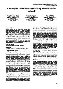
Also the single variable equation with as variable parameter has the least error toward the single variable relations in the past. (RMSE=0.044, MAPE=17.12, MAD=0.0352 and = 0.96)(Equation 2 in Table 4 and Figure 2. (Figures 1 and 2 show the relationship between output targets and predicted values obtained from the proposed relationships (R, Coefficient of Correlation). It can be seen that the proposed equation results in points more closely located around the 1:1 line.
(5) Development of the ANN model Where, n is the number of data points,
and
are
respectively the actual measured and predicted output th value from the i output. The lower the RMSE, MAPE and MAD values, the better the model performance. Under ideal conditions an accurate and precise method gives of 1.0, RMSE, MAPE and MAD of 0. In Table 3, the RMSE, MAPE, MAD and of empirical equations are compared for all data sets collected in this study (400 data sets). It can be seen that the multi variable equation proposed by Azzouz et al. (1976) using , and as predictor variables gave the lowest RMSE value (0.0428), the lowest MAPE value (16.51), the lowest MAD value
In order to develop the artificial neural network (ANN) model, it is common practice to divide the available data into two subsets: training set to construct the ANN model and an independent validation set to estimate model performance. We divided the data set randomly into two separate data sets—the training data set (90% of the total data set) and the testing data set (10% of the total data set). In this study, among 400 data sets, 40 randomly collected data sets were used in the testing stage and 360 data sets were used in the training stage. The five parameters, , , LL, PI and were included in the input layer of all ANN models (Table 5). The network uses the default Levenberg-Marquardt algorithm for training. In the training stage the application randomly
2838
Sci. Res. Essays
Table 2. Some widely used compression index equations.
Independent variable
Equation
Reference Single variable equation Azzouz et al. (1976) Koppula (1981) Herrero (1983b) Park and Lee (2011) Nishida (1956) Cozzolino (1961) Sower (1970) Park and Lee (2011) Azzouz et al. (1976) Bowles (1989) Ahadiyan et al. (2008) Hough (1957) Gunduz and Arman (2007) Azzouz et al. (1976) Mayne (1980) Terzaghi and Peck (1967) Park and Lee (2011) Bowles (1989) Multi-variable equation Nagaraj and Murthy (1985) Park and Lee (2011) Koppula (1981)
,
Azzouz et al. (1976) ,
(Azzouz et al. 1976)
,
Al-Khafaji and Andersland (1992) Ahadiyan et al. (2008)
,
Azzouz et al. (1976)
,
Yoon and Kim (2006) Herrero (1983a)
, , LL,
,
Ozer et al. (2008) Ozer et al. (2008)
divides input vectors and target vectors into three sets as follows:
3. The last 20% are used as a completely independent test of network generalization.
1. 60% are used for training. 2. 20% are used to validate that the network is generalizing and to stop training before over fitting.
In the present study feed forward with back-propagation neural network is utilized for data. MATLAB 7.6 is used in training and simulation of data. Various numbers of
Kalantary and Kordnaeij
Table 3. Statistical results for conventional empirical formulas (
Equation No
).
Equation
MAPE
RMSE
MAD
1
0.918
25.17
0.0629
0.0517
2
0.80
41.83
0.0975
0.086
3
0.937
21.26
0.0553
0.0437
4
0.85
33.79
0.0845
0.0695
5
0.93
21.27
0.0572
0.0437
6
0.95
18.63
0.0478
0.0383
7
0.86
29
0.0820
0.0596
8
0.87
31.46
0.0781
0.0647
9
0.96
17.32
0.0445
0.0356
10
0.80
39.31
0.0983
0.0808
11
0.957
17.5
0.0458
0.036
12
0.89
28.72
0.0723
0.059
13
0.30
95.38
0.2499
0.196
14
0.87
29.45
0.0792
0.0605
15
0.79
37.41
0.1012
0.0769
16
0.74
41.96
0.1111
0.0863
17
0.045
91.4
0.2244
0.188
18
0.81
36.81
0.0965
0.0757
19
0.84
33.42
0.0867
0.0687
20
0.6426
53.98
0.1313
0.111
21
0.3984
122.09
0.2597
0.251
22
0.92
24.87
0.0621
0.0511
23
0.95
18.326
0.0468
0.0377
24
0.95
19.17
0.0498
0.0394
25
0.95
17.7851
0.0492
0.0366
26
0.97
16.51
0.0428
0.0339
27
0.88
29.45
0.0766
0.0605
28
0.94
19.39
0.0538
0.0398
29
0.96
18.03
0.0455
0.0371
30
0.95
18.89
0.0475
0.0389
MAPE
RMSE
MAD
Table 4. Suggested empirical equations and statistical results.
Equation No
Equation
1
0.95
19.48
0.0513
0.04
2
0.96
17.12
0.044
0.0352
3
0.97
14.86
0.0385
0.0306
2839
2840
Sci. Res. Essays
Figure 1. The measured compression indexes obtained from the consolidation test versus the suggested equation estimated compression indexes (Equation 2, Table 4).
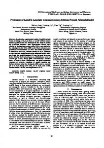
Figure 3. The measured compression indexes obtained from the consolidation test versus the ANN estimated compression indexes (result of training process).
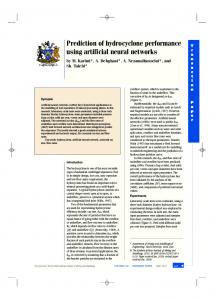
The combination of two hidden layers gives better results than single hidden layer and also the combination of transfer functions composed of log-sigmoid, tansigmoid and linear function gives good results. The ANN model with five neurons in the input layer, nine neurons in the first hidden layer, three neurons in the second hidden layer, and one node in the output layer gives the best results. Figures 3 and 4 shows the relationship between output targets and predicted values obtained through the training and testing process. The model shows very good correlation for both the training and testing data compared with the conventional empirical formulas and the suggested formulas. In Table 6, the predictability of the ANN model is statistically compared with the empirical formulas. The value of RMSE, MAPE and MAD are found to be minimum for the ANN model in both training and testing stage. Therefore, the developed ANN model is more efficient than the existing and proposed empirical formulas and by using it we can accurately estimate the consolidation settlement of this aria. Figure 2. The measured compression indexes obtained from the consolidation test versus the suggested equation estimated compression indexes (Equation 3, Table 4).
neuron in the hidden layer and the combinations of transfer functions were tested to find the optimal structure for the ANN model. The value of the minimum mean squared error, mean absolute percent error and mean absolute deviation were varied based on the correlation coefficient ( ) for the testing results.
Conclusion In this study, the performances of widely used single and multi-variable empirical equations for the estimation of the compression index were evaluated using a database consisting of 400 wide-ranging samples from the Province of Mazandaran, Iran. Using the same database, new single and multi-variable empirical equations were developed. Furthermore, an attempt has been made to predict this index by using neural network simulation. The
Kalantary and Kordnaeij
2841
Table 5. Descriptive statistics of variables used in the ANN.
Variable
Input
Mean 0.357 LL PI
Output = natural water content (%),
Test (40 data set) maximum minimum 1.882 0.767
Train (360 data set) Maximum minimum 1.647 0.769
mean 0.476
10.2
70
28.51
14.5
64.1
29.47
24 3 2.43
81 50 2.8
39.9 18.68 2.64
27 7 2.44
64 35 2.74
39.15 17.85 2.62
0.05
0.628
0.2054
0.076
0.53
0.2067
= initial void ratio, LL= liquid limit (%), PI= plastic index (%),
= specific gravity of soil particles,
= compression index.
Figure 4. The measured compression indexes obtained from the consolidation test versus the ANN estimated compression indexes (result of testing process).
Table 6. Statistical results for the best empirical formulas and ANN.
Equation No
Equation
MAPE
RMSE
MAD
1
, Herrero (1983) [12]
0.937
21.26
0.0553
0.0437
2
, in this study
0.95
19.48
0.0513
0.04
0.96
17.32
0.0445
0.0356
0.96
17.12
0.044
0.0352
0.97
16.51
0.0428
0.0339
0.97
14.86
0.0385
0.0306
, Azzouz et al. (1976) [10]
3
, in this study
4
, Azzouz et al. (1976) [10]
5 6
, this study
in
7
,
ANN model (training)
0.975
13.34
0.0348
0.0274
8
,
ANN model (testing)
0.978
13.17
0.0337
0.0272
2842
Sci. Res. Essays
results indicate that: 1. Among the single variable equations, the equation proposed by Azzouz et al. (1976) (Equation 9 in Table 3(, utilizing initial void ratio as the variable, has the lowest error. 2. Among the multi variable equations, the equation proposed by Azzouz et al. (1976) (Equation 26 in Table 3( gave the best performance using initial void ratio, natural water content and liquid limit of soil as predictor variables. 3. Based on the regression analysis, the formulas using single parameters of the void ratio and natural water content show better performance than other types of formulas using the single parameter. 4. The proposed equation using void ratio shows the lowest RMSE, MAPE, MAD and the highest regression coefficient which is better than the existing single variable equations. 5. Among the suggested equations, the equation shows the lowest RMSE value (0.0385), MAPE value (14.86), MAD value (0.0306) and the highest regression coefficient for the compression index. 6. The predictions of artificial neural network model agreed well with the measured compression index of the consolidation tests. Therefore, reliable predicting capabilities were obtained. 7. The developed ANN model is more efficient than the existing and proposed empirical formulas and by using it we can accurately estimate the consolidation settlement of this aria. ACKNOWLEDGEMENTS Authors are thankful to engineers Afshin Khatami, Mohsen Taheri and Hadi Shirsavar for their help. Authors also thank the Technical and Soil Laboratory of Mazandaran Province for collecting the borehole data. REFERENCES Abedimahzoon N, Molaabasi H, Lashtehneshaei MA, Biklaryan M (2010). Investigation of undertow in reflective beaches using a GMDH-type neural network. Turk. J. Eng. Environ. Sci. 34:201-213. Ahadiyan J, Ebne JR, Bajestan MS (2008). Prediction Determination of Soil Compression Index, Cc, in Ahwaz Region (In Persian). J. Faculty Eng. 35(3):75-80. Al-Khafaji AWN, Andersland OB (1992). Equations for compression index approximation. J. Geotech. Eng. ASCE. 118(1):148-153. ASTM D 2435-96 (1998). Standard Test Method for One-dimensional Consolidation Properties of Soils, Annual Book of ASTM standards. Vol. 04.08, Soil and Rock (I). Standard. Pennsylvania pp.207-216. Azzouz AS, Krizek RJ, Corotis RB (1976). Regression Analysis of Soil Compressibility. Soils Found. 16(2):19-29. Bowles JE (1989). Physical and Geotechnical Properties of Soils. McGraw-Hill Book Company Inc. New York, pp. 442-448. Cho SE (2009). Probabilistic stability analyses of slopes using the ANNbased response surface. Comput. Geotech. 36:787-797. Cozzolino VM (1961). Statistical forecasting of compression index. In: Proceedings of the fifth international conference on soil mechanics
and foundation engineering. Paris pp.51-53. Das BM (2009). Principles of geotechnical engineering. 7nd edition. Thomson Engineering p. 294. Du JC, Zhang LM (2001). Simplified Procedure for Estimating Ground Settlement under Embankments. In: Third International Conference on Soft Soil Engineeringc. Hong Kong pp.193-198. Fenton GA, Paice GM, Griffiths DV (1996). Probabilistic Analysis of Foundation Settlement. Proceedings of the ASCE Uncertainty. 96 Conference. Madison. Wisconsin. Aug. ASCE Geotechnical Special Publication 58(1):657-665. Goktepe F, Arman H, Pala M (2010). A new approach for classification of clayey soil: A case study for Adapazari region, Turkey. Sci. Res. Essays 5(15):2037-2043. Gunduz Z, Arman H (2007). Possible Relationships between Compression and Recompression Indices of a Low–Plasticity Clayey Soil. Arab. J. Sci. Eng. 32(2B):179-189. Haykin S (1999). Neural Networks. A Comprehensive Foundation (2nd edn). Prentice-Hall: Upper Saddle River. New Jersey. Herrero OR (1983a). Universal compression index equation. Discussion. J. Geotech. Eng. Div. ASCE. 109(10):1179-1200. Herrero OR (1983b). Universal compression index equation. Closure. J. Geotech. Eng. Div. ASCE. 109(5):755-761. Hornig ED (2010). Field and Laboratory Tests Investigating Settlements of Foundations on Weathered Keuper Marl. Geotech. Geol. Eng. 28:233-240. Hough BK (1957). Basic Soils Engineering. The Ronald Press Company. New York pp.114-115. Kolay PK, Rosmina AB, Ling NW (2008). Settlement Prediction of Tropical Soft Soil by Artificial Neural Network (ANN). The 12th International Conference of International Association for Computer Methods and Advances in Geomechanics (IACMAG) pp.1843-1848. Koppula SD (1981). Statistical estimation of compression index. Geotech. Test. J. 4(2):68-73. Lambe TW (1976). Stress Path Method. JSMFD. ASCE. (SM6) 93:309331. Mayne PW (1980). Cam-clay predictions of undrained strength. J. Geotech. Eng. Div. ASCE. 106(11):1219-1242. Mollahasani A, Alavi AH, Gandomi AH, Rashed A (2011). Nonlinear Neural-Based Modeling of Soil Cohesion Intercept. KSCE. J. Civ. Eng. 15(5):831-840. Nagaraj TS, Murty BRS (1985). Prediction of the preconsolidation pressure and recompression index of soils. Geotech. Test. J. 8(4):199-202. Nishida Y (1956). A brief note on compression index of soils. J. SMFE. Div. ASCE. 82(3):1-14. Ozer M, Isik NS, Orhan M (2008). Statistical and neural network assessment of the compression index of clay-bearing soils. Bull. Eng. Geol. Environ. 67(4):537-545. Park HI (2010). Development of neural network model to estimate the permeability coefficient of soils. Marine Geosourc. Geotechnol. 29(4):267-278. Park HI, Cho CH (2010). Neural Network Model for Predicting the Resistance of Driven Piles. Marine Geosources and Geotechnol. 28(4):324-344. Park HI, Keon GC, Lee SR (2009). Prediction of Resilient Modulus of Granular Subgrade Soils and Subbase Materials Based on Artificial Neural Network. Road Mater. Pavement Design. 10(3):647- 665. Park HI, Kim YT (2010). Prediction of Strength of Reinforced Lightweight Soil Using an Artificial Neural Network. Int. J. ComputerAided Eng. 28(5):600-615. Park HI, Lee SR (2011). Evaluation of the compression index of soils using an artificial neural network. Comput. Geotech. 38(4):472-481. Sinan N (2009). Estimation of swell index of fine grained soils using regression equations and artificial neural networks. Sci. Res. Essays 4(10):1047-1056. Sower GB (1970). Introductory soil mechanics and foundation. 3rd ed. London: The Macmillan Company of Collier-Macmillan Ltd. p.102. Terzaghi K (1925). Erdbaumechanik auf bodenphysikalischer Grundlage F. Deuticke. Terzaghi K, Peck RB (1967). Soil mechanics in engineering practice. 2nd ed. New York: Wiley p. 73. Wakita E (1993). Settlement Prediction Using Observed Data and Its
Kalantary and Kordnaeij
Feedback to Original Design. Proc. of the Intl. Conf. on Soft Soil Engineering. Edited by Cheung YK, Yuan JX, Lu PY, Tsui Y, Cao H. Guangzhou. China. Nov. Recent Adv. Soft Soil Eng. pp.92-97. Yoon GL, Kim BT (2006). Regression Analysis of Compression Index for Kwangyang Marine Clay. KSCE. J. Civ. Eng. 10(6):415-418.
2843
2844
Sci. Res. Essays
Appendix 1
33.6 26.2 30.5 19.2 32.5 30.2 39.1 55.7 34.5 36.5 36.2 22.5 12.7 22.4 20.8 24.5 25.7 26.6 44.4 40.3 48.1 32.7 26.7 27.7 28.6 47.6 27.4 18.7 39.1 25.9 27.6 24.4 28.6 31.1 21.6 28.8 20 21.3 25.2 22.1 22.4 20 17.2 19.4 31.2 23.7
LL 33 46 37 34 40 41 67 60 75 62 58 25 31 27 30 31 46 27 42 42 40 44 40 36 41 42 27 34 49 36 37 38 35 30 39 36 36 27 42 34 58 40 43 44 50 40
Appendix 1. Contd.
PI 13 24 18 15 20 22 43 32 47 34 33 5 10 8 10 12 23 7 20 19 19 22 19 14 17 21 6 13 24 13 16 14 14 10 21 17 20 17 20 13 32 19 21 21 29 21
0.789 0.666 0.853 0.706 0.793 0.777 0.939 1.357 0.828 0.959 0.894 0.595 0.63 1 0.508 0.748 0.722 0.766 1.148 1.04 1.286 0.859 0.669 0.677 0.702 1.135 0.68 0.711 0.948 0.762 0.748 0.613 0.764 0.856 0.552 0.759 0.562 0.547 0.645 0.66 0.685 0.605 0.73 0.576 0.74 0.585
Gs 2.6 2.7 2.67 2.5 2.65 2.68 2.55 2.54 2.58 2.72 2.63 2.64 2.62 2.67 2.69 2.61 2.63 2.66 2.7 2.73 2.72 2.64 2.67 2.63 2.58 2.63 2.66 2.66 2.6 2.7 2.61 2.53 2.62 2.68 2.6 2.64 2.61 2.64 2.6 2.6 2.61 2.6 2.7 2.7 2.52 2.6
Cc 0.28 0.126 0.26 0.196 0.186 0.219 0.36 0.5 0.27 0.375 0.32 0.183 0.236 0.196 0.05 0.266 0.199 0.149 0.26 0.27 0.322 0.216 0.133 0.136 0.146 0.37 0.163 0.22 0.32 0.103 0.236 0.13 0.3 0.25 0.11 0.21 0.163 0.103 0.159 0.173 0.153 0.196 0.206 0.11 0.259 0.22
37.5 29.7 25.9 24.1 21.6 25.3 27.1 31.4 30.8 30.8 22.4 19.5 27.1 28.9 39 25.3 25.2 26.7 29.7 22.6 36.5 29.4 27.1 24.7 24.4 48.7 36.9 22.6 31.9 27.2 24.7 25.3 26 26.9 21.8 32 40.9 23.5 57.4 31.1 32.2 38.1 29.8 27.5 22.1 31.8
LL 47 36 31 27 34 34 37 29 35 25 53 52 45 52 53 35 40 29 30 33 49 52 45 29 40 25 56 56 39 33 34 27 37 42 38 51 37 35 79 43 30 42 47 34 34 37
PI 24 14 11 8 12 13 14 7 13 5 28 28 22 28 29 14 18 8 10 10 28 28 22 11 22 5 28 34 17 14 13 8 17 20 17 32 10 15 45 22 10 20 27 15 14 16
0.915 0.753 0.736 0.675 0.83 0.734 0.72 0.839 0.825 0.869 0.583 0.517 0.652 0.806 0.98 0.675 0.588 0.663 0.718 0.632 0.97 0.731 0.809 0.71 0.695 1.222 0.909 0.612 0.837 0.677 0.745 0.661 0.723 0.716 0.563 0.829 0.928 0.507 1.587 0.964 0.782 0.87 0.736 0.739 0.573 0.776
Gs 2.6 2.63 2.63 2.67 2.59 2.61 2.65 2.68 2.71 2.69 2.6 2.61 2.6 2.55 2.63 2.7 2.6 2.67 2.66 2.64 2.62 2.62 2.72 2.63 2.7 2.59 2.57 2.68 2.68 2.66 2.67 2.66 2.59 2.58 2.67 2.59 2.53 2.52 2.53 2.65 2.62 2.51 2.57 2.72 2.59 2.65
Cc 0.29 0.2 0.21 0.126 0.28 0.2 0.176 0.15 0.2 0.2 0.169 0.14 0.18 0.28 0.26 0.13 0.16 0.12 0.11 0.116 0.29 0.22 0.22 0.19 0.123 0.41 0.27 0.15 0.2 0.17 0.18 0.156 0.21 0.216 0.103 0.31 0.31 0.11 0.628 0.365 0.159 0.256 0.25 0.146 0.123 0.166
Appendix 1. Contd. Appendix 1. Contd.
27.3 27.4 27.2 28.1 22.1 24.5 29.6 11.5 17.6 18.5 19.2 13.6 35.3 32.1 32.4 32.8 30.5 30.3 31.4 34 28.5 25.6 28.3 30.8 26.7 24.8 22 27.6 41.1 49.2 34.8 27.2 37.8 38.4 35.3 28 29 38.7 29.8 34 26.5 25.1 30.3 19.4 22.5 20.3
LL 37 36 31 34 43 39 37 45 52 46 51 46 35 49 48 49 38 42 41 33 39 35 37 32 44 26 24 37 39 60 51 36 44 62 41 37 39 53 54 58 36 43 46 38 36 30
PI 18 14 11 12 21 19 15 22 28 23 25 22 13 29 28 28 17 20 22 16 19 16 17 14 22 6 4 15 17 36 27 19 24 44 20 17 19 30 31 36 17 25 25 17 16 8
0.802 0.777 0.769 0.824 0.643 0.761 0.761 0.537 0.615 0.611 0.586 0.407 0.841 0.805 0.85 0.797 0.79 0.755 0.816 0.894 0.725 0.803 0.734 0.813 0.667 0.704 0.558 0.873 0.993 1.008 0.854 0.678 0.965 1.014 0.909 0.721 0.77 0.833 0.755 0.867 0.676 0.708 0.775 0.529 0.599 0.546
Gs 2.74 2.63 2.65 2.66 2.56 2.62 2.66 2.63 2.56 2.62 2.63 2.62 2.61 2.61 2.65 2.61 2.62 2.63 2.68 2.62 2.64 2.62 2.64 2.63 2.67 2.7 2.64 2.64 2.63 2.63 2.57 2.66 2.69 2.61 2.69 2.71 2.68 2.61 2.57 2.61 2.62 2.6 2.63 2.64 2.63 2.64
Cc 0.179 0.229 0.176 0.269 0.203 0.183 0.173 0.13 0.21 0.173 0.186 0.113 0.256 0.233 0.249 0.309 0.249 0.193 0.266 0.329 0.183 0.203 0.159 0.272 0.123 0.226 0.103 0.329 0.259 0.249 0.249 0.153 0.229 0.326 0.226 0.163 0.279 0.302 0.149 0.196 0.159 0.156 0.173 0.11 0.149 0.149
Kalantary and Kordnaeij
21.7 19.4 22.9 25.3 28.4 23.7 29.1 39.8 28.6 24.9 27.2 20.9 21 25 29.8 31.1 26.3 25.1 25.8 30.1 26.9 23.9 28.9 28.5 27 29.7 24.3 28.4 24.4 25.1 26.4 26.2 22.6 27.5 28 25.7 23.2 23.1 27 22.4 32.7 28.8 29.8 29 27.3 18.6
2845
2846
LL 42 40 31 31 36 34 34 53 46 33 34 30 25 36 43 30 60 37 39 39 43 30 26 39 44 32 42 29 31 29 31 30 30 31 33 32 35 31 32 27 57 56 31 43 58 32
PI 22 19 12 11 16 15 13 27 22 14 13 13 9 15 19 10 30 16 17 19 20 8 8 20 24 11 24 9 15 11 14 15 10 7 12 10 13 11 10 6 35 36 11 22 35 13
0.658 0.528 0.628 0.723 0.732 0.761 0.748 0.97 0.801 0.69 0.759 0.601 0.643 0.697 0.828 0.874 0.733 0.738 0.73 1.012 0.732 0.605 0.824 0.653 0.629 0.822 0.809 0.777 0.711 0.658 0.619 0.746 0.602 0.738 0.703 0.718 0.652 0.635 0.644 0.643 0.904 0.793 0.831 0.798 0.807 0.645
Sci. Res. Essays
Gs 2.6 2.53 2.57 2.62 2.63 2.66 2.66 2.64 2.77 2.77 2.76 2.76 2.74 2.72 2.72 2.72 2.72 2.67 2.64 2.52 2.63 2.53 2.74 2.53 2.51 2.76 2.76 2.73 2.66 2.7 2.64 2.8 2.67 2.66 2.68 2.71 2.68 2.66 2.44 2.66 2.76 2.75 2.72 2.74 2.72 2.72
Cc 0.22 0.149 0.143 0.169 0.176 0.189 0.213 0.252 0.153 0.13 0.163 0.11 0.103 0.183 0.186 0.209 0.196 0.203 0.196 0.4 0.163 0.133 0.199 0.186 0.166 0.213 0.199 0.14 0.159 0.149 0.14 0.183 0.13 0.173 0.103 0.166 0.206 0.146 0.196 0.189 0.282 0.246 0.176 0.209 0.229 0.14
Appendix 1. Contd.
25.6 31.2 29.8 25.2 26.4 20 22.7 31.4 25.2 29.5 29.3 30.8 29.8 34 26.5 30.3 23.9 26.9 23.9 28.9 33.6 26.2 11.1 20.5 24.1 31.4 36.6 32.1 28.9 34.4 19.9 20.2 23.1 16.6 23.2 22 35.4 36.2 31.9 27.6 28.9 28.1 29.8 28.3 35 23.8
LL 48 54 47 35 39 27 29 33 34 33 29 28 54 58 36 46 31 43 30 26 33 46 27 29 34 47 35 29 47 49 52 56 53 37 61 34 38 39 33 40 36 43 34 58 57 39
PI 25 30 26 16 19 9 7 10 12 9 7 5 31 36 17 25 12 20 8 8 13 24 5 8 12 29 15 7 26 28 31 36 35 21 37 13 19 17 12 18 15 20 14 35 34 16
Appendix 1. Contd.
0.724 0.776 0.785 0.663 0.667 0.63 0.637 0.768 0.675 0.784 0.795 0.751 0.755 0.867 0.676 0.775 0.621 0.732 0.605 0.824 0.789 0.666 0.519 0.717 0.668 0.826 0.883 0.753 0.717 0.864 0.582 0.498 0.642 0.507 0.586 0.675 0.859 0.881 0.705 0.666 0.711 0.719 0.753 0.692 0.88 0.828
Gs 2.64 2.63 2.64 2.65 2.55 2.59 2.7 2.45 2.67 2.66 2.71 2.62 2.57 2.6 2.62 2.63 2.61 2.63 2.53 2.74 2.6 2.7 2.58 2.71 2.71 2.64 2.59 2.6 2.64 2.61 2.59 2.43 2.53 2.56 2.55 2.54 2.56 2.63 2.67 2.67 2.66 2.67 2.66 2.57 2.61 2.72
Cc 0.163 0.183 0.173 0.14 0.279 0.193 0.183 0.252 0.229 0.143 0.186 0.173 0.149 0.196 0.159 0.173 0.156 0.163 0.133 0.199 0.279 0.126 0.126 0.146 0.106 0.179 0.246 0.213 0.246 0.223 0.166 0.169 0.169 0.226 0.159 0.216 0.249 0.252 0.12 0.156 0.216 0.156 0.183 0.159 0.256 0.159
21.3 20.6 18.5 10.6 26.1 20.1 19.7 21.9 28.8 33.7 28.7 28.2 30.1 27.6 30.8 26.5 21.3 26.3 20.4 26.1 19.5 19 18.4 18.4 49.6 40.6 39 31.2 36.1 33 32.7 34.4 30.9 37.4 27.1 33.6 31.4 29 25.6 31.2 25.3 23.3 25.3 25.3 29 35.3
LL 36 26 36 24 31 49 45 51 44 36 40 40 29 34 37 29 41 24 32 30 28 40 37 34 55 37 58 34 56 37 62 62 40 55 59 46 41 39 48 54 39 25 30 39 39 44
PI 12 9 15 3 12 25 22 26 22 14 20 18 10 16 15 8 20 4 11 11 9 19 17 15 28 16 35 14 34 15 36 36 21 30 36 24 22 20 25 30 21 6 9 21 20 23
0.502 0.551 0.567 0.368 0.778 0.638 0.661 0.694 0.75 0.844 0.755 0.757 0.75 0.738 0.784 0.637 0.699 0.695 0.699 0.752 0.73 0.715 0.682 0.613 1.322 1.088 1.059 0.871 0.983 0.88 1.054 0.806 0.926 0.921 0.693 0.847 0.804 0.748 0.724 0.776 0.647 0.579 0.702 0.647 0.748 0.815
Gs 2.52 2.61 2.63 2.65 2.64 2.7 2.7 2.71 2.67 2.64 2.55 2.6 2.62 2.7 2.61 2.63 2.68 2.68 2.7 2.71 2.7 2.63 2.62 2.63 2.67 2.69 2.7 2.73 2.7 2.67 2.62 2.56 2.59 2.6 2.61 2.64 2.63 2.59 2.64 2.63 2.61 2.65 2.53 2.61 2.59 2.54
Cc 0.11 0.159 0.106 0.09 0.189 0.09 0.149 0.156 0.209 0.203 0.249 0.169 0.223 0.189 0.199 0.166 0.14 0.169 0.173 0.183 0.113 0.219 0.213 0.153 0.409 0.259 0.385 0.176 0.306 0.209 0.355 0.312 0.379 0.246 0.259 0.296 0.229 0.233 0.163 0.183 0.259 0.093 0.189 0.259 0.233 0.183
Appendix 1. Contd.
24.6 29 25.8 27.8 26.7 54.3 28.3 29.5 27.7 20.5 23.4 21.6 21.9 20.5 25.3 20 70 37.8 37.1 10.2 44 40.1 43 27.2 37.2 27.9 34.4 24.4 37 28.2 39.6 27.1 28.5 23 25.1 27.4 20.5 29.8 21.4 22.2 43.4 21.6 28.8 24.5 56.9 22.2
LL 34 40 34 33 38 30 34 32 35 42 45 42 44 47 55 46 52 81 27 44 47 46 53 33 62 35 68 32 40 47 49 41 27 53 39 33 34 43 38 50 44 39 36 39 36 42
PI 14 19 12 10 18 10 13 14 15 21 21 23 24 22 27 25 29 50 6 23 23 23 31 8 34 15 46 14 19 24 25 18 7 28 16 12 13 24 21 27 21 21 17 19 15 21
0.676 0.8 0.692 0.707 0.684 0.943 0.778 0.744 0.73 0.601 0.697 0.664 0.686 0.742 0.719 0.671 1.882 0.966 0.951 0.357 1.137 0.996 1.062 0.881 0.937 0.745 0.909 0.824 0.923 0.814 0.891 0.666 0.735 0.608 0.672 0.727 0.565 0.789 0.583 0.614 0.994 0.552 0.759 0.644 1.442 0.568
Appendix 1. Contd.
Gs 2.63 2.64 2.63 2.63 2.62 2.67 2.68 2.65 2.68 2.6 2.67 2.58 2.59 2.56 2.63 2.61 2.68 2.67 2.69 2.62 2.69 2.66 2.64 2.61 2.56 2.67 2.44 2.66 2.63 2.717 2.611 2.633 2.67 2.55 2.65 2.62 2.7 2.59 2.68 2.62 2.51 2.6 2.64 2.7 2.68 2.6
Cc 0.225 0.279 0.173 0.176 0.179 0.282 0.133 0.173 0.159 0.229 0.176 0.156 0.166 0.196 0.209 0.176 0.54 0.27 0.25 0.08 0.39 0.33 0.4 0.266 0.345 0.153 0.226 0.276 0.309 0.2 0.26 0.116 0.173 0.16 0.13 0.17 0.076 0.22 0.15 0.166 0.302 0.11 0.206 0.176 0.405 0.153
Kalantary and Kordnaeij
31.8 29.6 31 33.3 42.2 38.2 26.1 24.7 22.4 22.2 16.4 19.4 25 29.7 32.1 30.2 25.4 23.6 17.7 41.5 47.6 46.6 36.5 25.9 33.5 23.5 33.7 21.6 30.6 32.1 28.7 40.7 33.1 29.9 38.5 28 39.3 39.4 28.9 28.9 28.9 20.1 23.8 28 34.5 25.2
2847
2848
LL 36 25 32 39 34 31 29 29 57 42 41 29 29 29 39 40 30 38 32 31 36 43 33 33 50 37 36 32 41 44 43 40 50 48 68 42 40 32 27 57 47 26 46 33 45 30
PI 16 6 11 20 13 11 9 8 33 19 24 11 9 11 20 22 10 19 12 11 17 22 12 12 26 16 15 12 17 26 16 18 27 25 42 24 17 8 6 35 25 8 25 12 26 11
0.831 0.834 0.786 0.868 1.161 0.967 0.786 0.763 0.697 0.534 0.605 0.495 0.691 0.778 0.823 0.787 0.644 0.592 0.74 1.195 1.237 1.127 0.934 0.8 0.827 0.596 0.835 0.665 0.727 0.761 0.82 1.045 0.771 0.756 0.884 0.657 0.931 0.979 0.817 1.031 1.137 0.676 0.647 0.703 0.808 0.681
Sci. Res. Essays
Gs 2.67 2.74 2.64 2.62 2.69 2.68 2.67 2.67 2.64 2.49 2.61 2.61 2.66 2.67 2.69 2.59 2.68 2.6 2.65 2.73 2.74 2.64 2.69 2.61 2.65 2.71 2.67 2.69 2.6 2.57 2.71 2.66 2.66 2.65 2.56 2.54 2.62 2.67 2.66 2.61 2.54 2.65 2.63 2.68 2.5 2.63
Cc 0.206 0.229 0.216 0.252 0.219 0.266 0.209 0.259 0.143 0.136 0.173 0.123 0.149 0.196 0.236 0.219 0.12 0.13 0.159 0.259 0.299 0.269 0.213 0.266 0.296 0.05 0.166 0.166 0.173 0.199 0.12 0.259 0.176 0.163 0.322 0.209 0.209 0.266 0.176 0.306 0.402 0.113 0.123 0.103 0.319 0.163
Appendix 1. Contd.
20 19.5 31.2 23.9 34.2 21.6 28.8 25.5 45.7 42.1 39.2 35 24.6 64.1 31 25.2 14.5 22.6 27.2 23 20.5 22.8 46.4
LL 34 34 37 31 44 39 32 29 52 34 57 37 34 64 33 56 44 28 29 37 32 28 31
PI 13 12 16 12 25 21 11 9 31 10 34 14 14 31 15 35 21 7 10 16 11 7 10
0.693 0.609 0.87 0.621 0.816 0.552 0.703 0.643 1.132 1.013 1.091 0.928 0.676 1.647 0.786 0.569 0.476 0.598 0.77 0.541 0.557 0.619 1.232
Gs 2.64 2.57 2.73 2.61 2.54 2.61 2.64 2.56 2.64 2.59 2.65 2.71 2.63 2.57 2.63 2.44 2.64 2.65 2.74 2.52 2.64 2.63 2.57
= natural water content (%), ratio, LL= liquid limit (%), PI= plastic index (%), particles,
Cc 0.183 0.189 0.209 0.156 0.239 0.11 0.206 0.126 0.379 0.355 0.302 0.233 0.226 0.53 0.193 0.146 0.126 0.173 0.183 0.106 0.106 0.153 0.465
= initial void
= specific gravity of soil
= compression index.