Jun 19, 2006 - subdominant during early stages of preheating, but it actually amplifies parametric resonance ...... four-legs interactions during the linear stage.
UMN-TH-2431/06
Preheating with Trilinear Interactions: Tachyonic Resonance 1
arXiv:hep-ph/0602144v2 19 Jun 2006
2
J.F. Dufaux1 , G.N. Felder2 , L. Kofman1 , M. Peloso3, D. Podolsky1∗
CITA, University of Toronto, 60 St. George st., Toronto, ON M5S 3H8, Canada Department of Physics, Clark Science Center, Smith College Northampton, MA 01063, USA and 3 School of Physics and Astronomy, University of Minnesota, Minneapolis, MN 55455, USA (Dated: February 2, 2008)
We investigate the effects of bosonic trilinear interactions in preheating after chaotic inflation. A trilinear interaction term allows for the complete decay of the massive inflaton particles, which is necessary for the transition to radiation domination. We found that typically the trilinear term is subdominant during early stages of preheating, but it actually amplifies parametric resonance driven by the four-legs interaction. In cases where the trilinear term does dominate during preheating, the process occurs through periodic tachyonic amplifications with resonance effects, which is so effective that preheating completes within a few inflaton oscillations. We develop an analytic theory of this process, which we call tachyonic resonance. We also study numerically the influence of trilinear interactions on the dynamics after preheating. The trilinear term eventually comes to dominate after preheating, leading to faster rescattering and thermalization than could occur without it. Finally, we investigate the role of non-renormalizable interaction terms during preheating. We find that if they are present they generally dominate (while still in a controllable regime) in chaotic inflation models. Preheating due to these terms proceeds through a modified form of tachyonic resonance.
I.
INTRODUCTION
According to the inflationary scenario, the universe at early times expands quasi-exponentially in a vacuum-like state without entropy or particles. During this stage of inflation, all energy is contained in a classical slowly moving inflaton field. Eventually the inflaton field decays and transfers all of its energy to relativistic particles, which starts the thermal history of the hot Friedmann universe. Particle creation in preheating, described by quantum field theory, is a spectacular process where all the particles of the universe are created from the classical inflaton. In chaotic inflationary models, soon after the end of inflation the almost homogeneous inflaton field coherently oscillates with a very large amplitude of the order of the Planck mass around the minimum of its potential. Due to its interactions with other fields, the inflaton decays and transfers all of its energy to relativistic particles. If the creation of particles is sufficiently slow (for instance, if the inflaton is coupled only gravitationally to the matter fields) the decay products simultaneously interact with each other and come to a state of thermal equilibrium at the reheating temperature Tr . This gradual reheating can be treated with the perturbative theory of particle creation and thermalization [1]. However, for a wide range of couplings the particle production from a coherently oscillating inflaton occurs in the nonperturbative regime of parametric excitation [2, 3, 4, 5]. This picture, with variation in its details, is extended to other inflationary models. For instance, in hybrid inflation (including D-term inflation) the inflaton decay proceeds via a tachyonic instability of the inhomogeneous modes which accompany the symmetry breaking [6]. One consistent feature of preheating – non-perturbative copious particle production immediately after inflation – is that the process occurs far away from thermal equilibrium. The transition from this stage to thermal equilibrium occurs in a few distinct stages, each much longer than the previous one. First there is the rapid preheating phase, followed by the onset of turbulent interactions between the different modes. Our understanding of this stage comes from lattice numerical simulations [7] as well as from different theoretical techniques [8]. For a wide range of models, the dynamics of scalar field turbulence is largely independent of the details of inflation and preheating [9]. Finally, there is thermalization, ending with equilibrium. In general, the equation of state of the universe is that of matter when it is dominated by the coherent oscillations of the inflaton field, but changes when the inflaton decays into radiation-dominated plasma [10]. Most studies of preheating have focused on the models with φ2 χ2 four-legs interactions of the inflaton φ with another scalar field χ. A common feature of preheating is the production of a large number of inflaton quanta with non-zero momentum from rescattering, alongside with inflatons at rest. The momenta of these relic massive inflaton particles eventually would redshift out. However, the decay of inflaton particles through four-legs φφ → χχ processes in an expanding universe is never complete. Thus inflaton particles later on will have a matter equation of state and come to dominate the energy density, which is not an acceptable scenario. Therefore, to avoid this, we must include in the theory of reheating interactions of the type φχn , that allow the inflaton to decay completely, thus resulting in a radiation dominated stage. Trilinear interactions are the most immediate and natural interactions of this sort.
∗
On leave from Landau Institute for Theoretical Physics, 117940, Moscow, Russia
2 Trilinear interactions occur commonly in many theoretical models. Yukawa couplings, for example, lead to trilinear vertices with fermions. Three-legs decay via fermions was in fact the first channel of inflaton decay considered in early papers on inflation [1] within perturbation theory. It was later realized that even in the case of interaction with fermions the inflaton decay typically occurs via non-perturbative parametric excitations [11]. However, threelegs decay via intractions with bosons is expected to be a dominant channel (due to Pauli blocking for fermions). Gauge interactions lead to trilinear vertices with vector fields. Even if we restrict ourselves to scalar field interactions, trilinear interactions naturally appear in many contexts. 2 Consider for instance a chaotic inflation model with the effective potential V = ± 21 m2 φ2 + 41 λφ4 + g2 φ2 χ2 . The negative sign corresponds to spontaneous symmetry breaking φ → φ + σ , which results in a classical scalar field VEV σ = √mλ . The interaction term g 2 φ2 χ2 then gives rise to a trilinear vertex σg 2 φ χ2 along with the four-legs interaction. Spontaneous symmetry breaking naturally emerges in the new inflationary scenario. However, this results in a mass for the χ particles which is comparable to the inflaton mass. This complicates the bosonic decay of the inflaton after new inflation, see also [12]. One encounters the same problem for spontaneous symmetry breaking in chaotic inflation models. However, a very different picture appears for chaotic inflation in supersymmetric theories. Trilinear interactions occur also naturally P in supersymmetric theories. Typical superpotentials are constructed from P trilinear combinations of superfields, W = ijk λijk Φi Φj Φk . The cross terms in the potential V = i |Wi |2 then give rise to a three-legs interaction, in addition to a four-legs vertex. Besides many other advantages, supersymmetry is useful to protect the flatness of the inflaton potential from large radiative corrections. Therefore we will pay special attention to trilinear interactions in SUSY theories. In SUSY the strengths of the couplings of three-legs and four-legs interactions are tightly connected. The scalar field potentials that we consider in this paper, and their stability constraints, are discussed in Section II. In general, we expect the inflaton to decay simultaneously via all potential interactions: three-legs, four-legs etc. In many cases, notably in the supersymmetric case, the leading channel of inflaton decay during preheating is bosonic four-legs parametric resonance, as it was assumed in the earlier papers on preheating [3]. In this case, parametric resonance is actually amplified by the trilinear interaction, as we show in Section IV. To reach this important conclusion, we shall understand how preheating works with a three-legs interaction. For this we shall consider an idealized situation when other interactions are switched off. To get an insight into how preheating occurs through a trilinear vertex 21 σφχ2 , consider the effective frequency of χ particles caused by the inflaton field φ(t) = Φ sin mt coherently oscillating around the origin ωχ2 (t) =
k2 + m2χ + σ φ (t) . a2
(1)
The bare mass of the χ will typically satisfy m2χ 0) is divided into stability and instability stripes (see, e.g. [15]). The line A = 2q divides the stability/instability chart into two regions. The case of parametric resonance for the four-legs interaction g 2 φ2 χ2 can be mapped onto the theory of stability/instability chart above the line A = 2q studied in [3]. The region below that line corresponds to what we call tachyonic resonance. On the formal side, we will extend the theory [3] of parametric resonance “below the line A = 2q”, which requires some new technical elements. The analytic theory of trilinear preheating will be constructed in Section III. In this paper, we study the effects of the trilinear φ χ2 interaction both during preheating and during the rescattering/early thermalization stage. Preheating produces a spectrum of particles predominantly in the infrared (low momentum) region. While 2 ↔ 2 interactions can lead to kinetic equilibrium, thermal equilibrium requires an increase of the average energy per particle, which in turn requires particle fusion. The beginning of particle fusion is already
3 visible during rescattering, as the simulations of [9] indicate. However, this process is expected to complete on time scales which are much longer than the ones we can run in a lattice simulation. Thermalization after preheating has been studied in detail only in limited intervals of time and momentum [9, 10, 16]. An analytic treatment of the dynamics of thermalization is possible only in the simplest cases, for instance, in the pure λ φ4 model [16], where the expansion of the universe can be scaled out and no mass scale appears. In an expanding universe in the more general case of a massive inflaton it is much harder to do analytically [9, 10]. If only quartic interactions are relevant, particle fusion proceeds most effectively by combining two vertices in a 4 → 2 process. If trilinear vertices are also present with comparable coupling strength, 3 → 2 processes become possible. Hence, trilinear vertices can be expected to play an important role in setting the thermalization time scale. Yukawa couplings can also be important for thermalisation, see e.g. [17] 1 . In Section V, we present the results of our numerical simulations and we discuss the effect of the trilinear interaction on the dynamics after preheating. We focus in particular on the evolution of the equation of state. As we already mentioned, during preheating four-legs interactions will often dominate over three-legs interactions. 1 2 3 In many cases we also may expect the presence of higher-order interactions like M χ φ , M12 χ2 φ4 , etc. These nonrenormalizable terms arise for example in supergravity theories. The cut-off scale M of the effective theory is expected to be close to the Planck scale. Planck-suppressed interactions are often supposed to lead only to perturbative contributions to reheating. The situation, however, may be very different for chaotic inflation because of the large inflaton amplitude right after inflation, Φ ∼ 0.1 MP . (Clearly, one has also to make sure that non-renormalizable terms do not affect the inflaton potential during inflation). In fact, surprisingly, non-renormalizable terms tend to Φ , where g 2 is the coupling of the four-legs dominate over renormalizable terms during preheating, as long as g 2 < M interaction. For M close to the Planck mass, Φ/M < 1 during preheating, and the effective mass squared of χ is then actually dominated by the φ3 χ2 /M interaction. This vertex leads to tachyonic growth of the quanta of χ, similar to what occurs with a three legs interaction. Note that the efficiency of this process is governed by the dimensionless parameter q ∼ Φ3 /(m2 M ), which is very large at the end of inflation. This also opens up the possibility of very efficient preheating even if the inflaton does not couple to the matter sector through renormalizable interactions2 . We consider tachyonic resonance due to non-renormalizable interactions in Section VI. We briefly summarize our results in section VII. II.
PROPERTIES OF POTENTIALS WITH TRILINEAR INTERACTIONS
In this section, we describe the models that we will consider in the following, and which are characterized by a trilinear interaction φχ2 between the massive inflaton φ and a light matter scalar field χ . In the presence of a φχ2 vertex (independently of the presence of a φ2 χ2 interaction), we have to include a χ4 self interaction as well for the potential to be bounded from below, and therefore stable. This means that there are several effects of the fields dynamics working simultaneously. We consider two examples of potentials with three-legs interactions, which stress different possibilities of preheating. 1) A simple potential which encodes the trilinear interaction between the massive inflaton φ and another scalar field χ is supplemented with a quartic self-interaction of χ but without a four-legs interaction φ2 χ2 V =
m2 2 σ λ φ + φ χ2 + χ 4 2 2 4
(2)
where σ has the dimension of mass. Here we assume that the bare mass of χ is negligible with respect to the inflaton mass. It is instructive to rewrite (2) in the form � � σ 2 �2 1 σ2 1 � mφ + λ− χ4 . (3) + χ V = 2 2m 4 2m2
Values λ < σ 2 /2m2 are not allowed, since in this case the potential is not bounded from below. The limiting case λ = σ 2 /2m2 is characterized by the exact flat direction φ = −σχ2 /2m2 where V = 0. The shape of the potential in this case is shown in Fig.1. Finally, for λ > σ 2 /2m2 the flat direction is lifted and the potential admits a single minimum at φ = χ = 0 where V = 0. For numerical estimates, we will often take λ = σ 2 /m2 in the following.
1 2
Trilinear interactions may also play an important role for electroweak baryogenesis and leptogenesis, see [18] and references therein If a Bose condensate associated with a flat direction forms during inflation, non-renormalizable interactions may also play an important role during preheating, as noticed in [19].
4
2 1
phi
0
5
-1 4 3 2 1
V
0 -1
-2 0 1
chi
FIG. 1: The potential (2) for λ = σ 2 /2m2 with an exact flat direction. For λ > σ 2 /2m2 the flat direction is lifted and the single minimum occurs at φ = χ = 0. Inflation occurs as φ rolls down the single valley at the top (positive φ) and preheating occurs as it oscillates between the single-valley and the double-valley.
The inflationary stage is driven by the φ-field in (2) if the effective mass of the χ field is large, i.e. if σ φ(t) > H 2 > m2 during inflation, and the χ field then stays at the minimum of its effective potential, at χ = 0. After inflation φ begins to oscillate around the minimum. We shall consider creation of particles of the test quantum field χ due to its trilinear interaction with the background oscillations of the classical field φ. When the inflaton passes the minimum of the potential, σ φ(t) becomes negative and χ acquires a negative mass squared around the local maximum in the χ-direction at χ = 0 (see Figure 1). As a result inhomogeneous quantum fluctuations of χ with momenta k 2 < |m2χ,eff (t)| = |σ φ(t)| grow exponentially with time, in a way similar to the tachyonic instability in hybrid inflation discussed in [6]. The difference here, however, is that tachyonic instability occurs only during the periods when the background field φ is negative and ceases during the parts of the φ oscillations when φ > 0. 2) We will also consider the potential V =
m2 2 σ g2 2 2 λ 4 φ + φ χ2 + φ χ + χ 2 2 2 4
(4)
with the additional four legs interaction. The potential is bounded from below for λ > 0. For 0 < λ < σ 2 /2m2 , the potential admits two minima at non vanishing φ and χ where V < 0. We mostly focus on the case λ ≥ σ 2 /2m2 , where there is a single minimum at φ = χ = 0 with V = 0. Close to this minimum the shape of the potential is similar to (2). The potential (4) may arise for instance from the superpotential g m W = √ φ2 + √ φ χ2 2 2 2 2
(5)
which gives λ = g 2 /2 and σ = gm (for the real part of χ). Preheating in the theory (4) occurs through a combination of effects due to the φ2 χ2 interaction and the φ χ2 interaction. In the Section IV we discuss the range of parameters for which the different interactions dominate. III.
ANALYTICAL THEORY OF TACHYONIC RESONANCE
In this section, we study the production of quanta of a scalar field χ whose effective mass squared periodically becomes negative in time due to its interaction with the classical inflaton field oscillating around its minimum. For definiteness, we consider the potential (2). The backreaction of the χ4 self-interaction is negligible during the early stage of preheating, so that only the φχ2 term is important.
5 The quantum field χ ˆ is decomposed into creation and annihilation operators with the eigenmodes χk (t) eik~x , where k is the co-moving momentum. After the usual rescaling χk → a3/2 χk , where a(t) is the scale factor of the (spatially flat) FRW universe, the temporal part of the χ-modes obeys the equation χ ¨k + ωk2 χk = 0 ,
(6)
where ωk2 =
k2 + σ φ(t) + ∆ , a2
(7)
∆ = −3a˙ 2 /4a2 − 3¨ a/2a, and a dot denotes a derivative with respect to the proper time t. The choice of the positive frequency asymptotic solution in the past fixes the initial conditions while the condition χk χ˙ ∗k − χ∗k χ˙ k = i fixes the normalization for the solution of equation (6). In this section we consider solutions of this equation for harmonically oscillating φ(t). Let us first neglect the expansion of the universe, a(t) = 1. The background solution for the inflaton is then given by φ(t) = Φ sin(mt) with a constant amplitude Φ. In this case, Eq.(6) reduces to the canonical Mathieu equation χ′′k + (Ak − 2q cos 2z)χk = 0
(8)
2
2σΦ where mt = 2z − π2 , Ak = 4k m2 and q = m2 , and a prime denotes the derivative with respect to z. Right after inflation 13 we have Φ0 ∼ 0.1 MP , while m ∼ 10 √ GeV in order to match with the observed CMB anisotropies. The q-parameter is then very large, for instance q0 ∼ λ 105 >> 1 for λ ∼ σ 2 /m2 . The stability/intsability chart (A, q) of the Mathieu equation is divided into bands. We are interested in unstable solutions, which correspond to the amplification of the vacuum fluctuations χk , in the regime of large q. Let us inspect the effective frequency ωk2 . Modes with momenta Ak ≥ 2q have positive ωk2 . We can view Eq.(6) as the Schrodinger equation with the periodic potential, where for Ak ≥ 2q the waves propagate above the potential barrier and are periodically scattered by its peaks. They are amplified at the instances when ωk2 is minimal, i.e. in the vicinity of z = lπ which corresponds to φ = −Φ in our case, and remain adiabatic outside of those instances. The whole process can be considered as a series of scatterings in a parabolic potential, which approximates ωk2 around its zeros. The net effect corresponds to broad parametric resonance, as described in [3]. However, for 0 < Ak < 2q the frequency squared of the modes with k 2 < σ Φ becomes negative during some intervals of time within each period of the background oscillations. These are the modes we consider in the rest of this section because they give the dominant contribution to the number of produced particles. For those, we still can use the method of successive scatterings, but each individual scattering cannot be approximated as scattering from a parabolic potential. This is where we have to modify the theory. Suppose the inflaton oscillations begin at some initial time t = t0 where ωk2 (t0 ) > 0 (take φ(t0 ) = Φ). Consider the period during the (j + 1)th oscillation of the inflaton, from t = tj to t = tj+1 where tj = t0 + 2π j/m. The frequency squared of the modes with k 2 < σ Φ is negative during a k-dependent interval
Ω2k (t) = −ωk2 (t) > 0
for
+ t− kj < t < tkj
(9)
+ 2 between the “turning points” t− kj and tkj where ωk = 0. Now we can view Eq.(6) with 0 < Ak < 2q as the Schrodinger equation with a periodic potential, where the wave periodically propagates above and below the potential barrier. Except in the vicinity of the turning points, we have |ω˙ k | 1, so we may use the WKB approximation to solve for (6). For t < t− kj (above the barrier), we have a superposition of positive- and negative-frequency waves � � � Z t � Z t αjk βkj j ′ ′ ′ ′ χk (t) ≃ χk (t) = p (10) ωk (t )dt + p ωk (t )dt exp −i exp i 2ωk (t) 2ωk (t) t0 t0
where the integral is taken over the intervals between t0 and t where wk2 > 0, and αjk and βkj are constant coefficients (in the adiabatic approximation) during this time interval, determined as we describe below. These correspond to the Bogoliubov coefficients (normalized as |αjk |2 − |βkj |2 = 1) and the initial vacuum for t → t0 is defined by the positive-frequency mode, α0k = 1, βk0 = 0. The adiabatic invariant njk = |βkj |2
(11)
corresponds to the occupation number of the χ-particles after j inflaton oscillations and will be the major object of interest.
6 + For t− kj < t < tkj (below the barrier), the WKB approximation gives a superposition of exponentially increasing and decreasing solutions ! ! Z t Z t bjk ajk ′ ′ ′ ′ exp − exp Ωk (t )dt + p (12) Ωk (t )dt χk (t) ≃ p 2Ωk (t) 2Ωk (t) t− t− kj kj
where ajk and bjk are constant coefficients (normalized as ajk bjk ∗ − ajk ∗ bjk = i). Finally, for t > t+ kj , we have χk (t) ≃ χj+1 (t) as given by (10) in the WKB regime with the shift j → j + 1 k The solution (12) with non-vanishing bjk corresponds to an exponentially fast prodution of particles. The WKB √ approximation in this tachyonic (below the barrier) stage is accurate for Ak < 2q −2 q. The duration of the tachyonic √ stage decreases with increasing k, that is with growing Ak . For 2q − 2 q < Ak < 2q there is a short tachyonic stage, during which however the WKB approximation does not apply. As Ak increases towards 2q, the χ-modes spend less √ and less time in the tachyonic regime, which becomes less and less efficient. For Ak > 2q − 2 q, particle production occurs in a small interval around φ = −Φ, providing a smooth limit with the case of broad parametric resonance for Ak ≥ 2q. To evaluate the growth of nk during one oscillation of the inflaton, we have to match between the successive approximate solutions (10) and (12) around the turning points, where the WKB approximation is inapplicable. This may be done by formally extending the domain of definition of χk to the complex plane, see Appendix A. Except for the normalization conditions, the procedure is similar to the calculation, in quantum mechanics, of the (spatial) evolution of a wave function in the quasi-classical regime [20]. We then find the “transfer matrix” between the Bogoliubov coefficients after and before the (j + 1)th oscillation of the inflaton3 αj+1 k βkj+1
!
=e
j
i e2iθk
1
Xkj
j
−i e−2iθk
1
!
αjk βkj
!
(13)
where Z
Xkj =
t+ kj
Ωk (t′ ) dt′
(14)
t− kj
R t− j kj 2 and θkj is the total phase accumulated from t0 to t− kj during the intervals where ωk > 0, θk = t0 dt ωk (t). When the expansion of the universe is neglected, Φ, t± k and Xk do not depend on j. We have furthermore in this case θkj = θk0 + j Θk where Θk =
Z
2π t− k + m
t+ k
ωk (t′ ) dt′
(15)
is the phase accumulated during one inflaton oscillation when ωk2 > 0. It is then easy to apply (13) (j + 1) times recursively. With the initial conditions α0k = 1 and βk0 = 0, one finds the occupation number of the χ-particles in the k-mode (with k 2 < σ Φ) after j oscillations of the inflaton to be njk = |βkj |2 = exp(2jXk ) (2 cos Θk )2(j−1) .
(16)
This simple formula is the main analytic result of our paper. exp (2 Xk ) gives the occupation number after the first oscillation. For the trilinear interaction (7), one finds from (14) and (15), in terms of the variables in the Mathieu equation (8) Xk =
3
Z
π+˜ zk π−˜ zk
� p Ωk (z) dz = 2 2q − Ak E z˜k ;
4q 2q − Ak
�
(17)
This may be expressed as� usual in terms of reflection and transmission coefficients satisfying |Rk |2 + |Dk |2 = 1, up to exponentially � small terms, ∝ exp −Xkj , which are beyond the accuracy of the WKB approximation.
7 and Θk =
Z
π−˜ zk
z˜k
p ωk (z) dz = 2 2q + Ak E
�
π 4q − z˜k ; 2 2q + Ak
�
where E(θ ; m) denotes the incomplete elliptic integral of the second kind with amplitude θ < [15]. Here we have defined � � π Ak 1 ∈ [0, ] z˜k = arccos 2 2q 4
(18) π 2
and parameter m
(19)
so that the turning points are given by zk± = π ± z˜k . The functional dependence of Xk , which controls the efficiency of particle production, is � � p Ak . Xk = 2 2q f 2q
(20)
In the interval we are interested (Ak < 2q), we found a good approximation f (y) ≃ 0.6 (1 − y) (verified numerically). Therefore, we can use the following accurate approximation x √ Xk ≃ − √ Ak + 2x q q
(21)
√
Γ(3/4) ≃ 0.85. with x = 2√π2 Γ(5/4) The analytic formula (16) derived with the WKB method, gives a pretty good approximation to the actual field dynamics. To show this, we plot in Figure 2 the occupation number njk in (16) as a function of Ak , after j = 1 and j = 4 oscillations, for the value of the parameter q = 20. Numerical calculations (dots) coincide with the results of the analytical curve.
Log@n_k1D
Log@n_k4D 60
14 12 10 8 6 4 2
40 20 5 10
20
30
40
A_k
10 15
20 25 30 35 40
A_k
-20
FIG. 2: log njk derived from (16) as a function of Ak , after j = 1 (left) and j = 4 (right) oscillations of the inflaton, for q = 20. The dots correspond to numerical solutions.
Quite interestingly, after several inflaton oscillations (j > 1), there are modes with negative frequency squared for which the tachyonic growth does not occur (see right panel of Figure 2). These form stability bands, which shrink to lines for q >> 1, given by cos Θk = 0 (see (16)). In some sense, the situation is reversed with respect to the conventional parametric resonance for q ≪ 1, where only some values of k, forming the instability bands, “resonate” with the frequency of the inflaton and undergo an exponential growth. Here, all the modes are amplified by the tachyonic instability except the ones belonging to the very narrow stability bands. These are described in more details in Appendix B. Beyond the WKB approximation, each stability line is split after each inflaton √ oscillation. After √ several oscillations, the net effect is the formation of stability bands of finite width δAk ∼ q e−x q . As q decreases, √ these bands become wider, while the distance between them decreases as ∆Ak ∼ q (see appendix B) ; at the same √ time the efficiency of particle production decreases as Xk ∼ q from (21)). When q < 1, the width of the stability and instability bands are comparable, and the tachyonic effect becomes indistinguishable from (narrow) parametric resonance (as is clear from the stability/instability chart of the Mathieu equation in this region of parameters).
8 The expansion of the universe can be incorporated “adiabatically”, which is to say that the above formulas will stay the same but the parameters will depend on a(t). In an expanding universe, we may essentially repeat the discussion √ √ ˙ leading to (13) without any modification, because of the hierarchy of scales Φ/Φ ∼ ∆ ∼ H |ωk |2 , is satisfied. This happens in small intervals 1/4 ∆ sin(mt) ∼ 2/q4 around sin(mt) = −q3 /2q4 , as may be found by applying the calculation of [3]. The typical √ q4 q32 k2 momentum of the modes amplified by this process is given by m 2 = 4q + 2 . Inspecting the right hand side of this 4 3/4
expression, we can break the range of q3 and q4 into two regions, q3 < q4 For the case 3/4
q3 < q4
3/4
and q3 > q4 . (28)
the periods of tachyonic instability are negligible, and particle production occurs due to the non-adiabaticity in very small intervals m ∆t q4
(31)
the tachyonic effect is dominant, and we have to use formula (16) of the previous section. √ We are especially interested in the SUSY case. Let us take the superpotential (5), which leads to q3 = q4 . For q3 , q4 ≫ 1 this corresponds to the case (28). This means that in the SUSY theory where both three and four legs interactions are present, the stage of preheating is dominated by the four legs interaction.
10 3/4
Suppose that initially we have condition (28), as in the SUSY theory. Consider q4 /q3 as function of time. The 3/4 inflaton amplitude redshifts as Φ ∼ (mt)−1 with the expansion of the universe, so that the critical ratio q4 /q4 decreases with time as (mt)−1/2 . If initially this ratio is larger than unity, it decreases with time and later on the 3/4 situation reverses, q4 /q4 becomes less than unity, and the three legs vertex dominates. We conclude that in many cases, notably in the SUSY theory, the stage of preheating is dominated by the effects of the four legs interaction, while the later stages are dominated by the three legs interaction. As we will see in the next section, independently of the dominant mechanism for preheating, the trilinear interaction dominates the following turbulent dynamics. V.
NON-LINEAR DYNAMICS AFTER PREHEATING WITH A THREE LEGS INTERACTION
So far we have analytically studied preheating with a three-legs interaction and compared the effects of three- and four-legs interactions during the linear stage. After the system becomes non-linear, the analytic theory is replaced by numerical simulations of the dynamics. In this section we report the results of those simulations. We will consider three different models, one with only a four-legs interaction, one with only a three-legs interaction, and one with both three- and four-legs interactions. Let us define these three models as Model A:
q4i = 104
Model B:
4
Model C:
q4i = 10 q4i = 0
, , ,
qχi = 5 × 10³
qχi = 5 × 10 qχi = 10
4
3
, , ,
q3i = 0
(32) 2
(33)
2
(34) (35)
q3i = 10 q3i = 10
where we have introduced the dimensionless quantities q4i = g 2 Φ20 /m2 , q3i = σΦ0 /m2 and Φ0 = 0.193 MP is the initial amplitude of the inflaton zero-mode at the end of inflation. The parameter qχi = λΦ20 /m2 characterizes the self-interaction of the χ-field. Model A is a standard preheating model with parametric resonance due to a four-legs interaction, without threelegs coupling. Model B contains both three- and four-legs couplings and corresponds to the SUSY case discussed in Section II with λ = g 2 /2 and σ = g m in (4). Model C corresponds to the potential (2) without φ2 χ2 interaction (when the exact flat direction shown in Figure 1 is slightly lifted, λ > σ 2 /(2m2 )) and thus allows us to see the pure effects of tachyonic resonance due to the three-legs coupling. A χ4 self-interaction is present in all models (to ensure the stability of the potential in the presence of the φ χ2 interaction, see Section II). We will see that this self-interaction does not change qualitatively the dynamics. We used the LATTICEEASY program [21] to perform numerical lattice simulations for the theory (4) in an expanding universe. For the three models, we used a 3-dimensional lattice with N = 2563 points and a comoving edge size L = 10/m. This allows us to probe comoving momenta in the range 0.6 m < k < 140 m. Here we are interested in the behavior of the system both during and after preheating. Long time integrations require both a high ultra-violet (UV) cutoff for the modes and a high resolution of modes in the infra-red (IR) part of the spectra. This motivates the value of q4i chosen, which is large enough to produce efficient preheating, but also small enough to produce quick rescattering [10]. For the three models, the simulations were performed up to a total period of m ∆t = 1000 starting from the end of inflation. We also checked the robustness of our results by performing 2-dimensional simulations with both a larger UV cutoff (smaller lattice spacing) and a higher resolution in the IR (larger box size). As output of the calculations, we present the evolution of the mean values of the fields, the evolution of the occupation number spectra, and most importantly the evolution of the equation of state. For the definitions of these quantities, see e.g. [10]. As we will see, after the preheating stage model B (with both types of interactions) will behave qualitatively similarly to model C (with only a three legs interaction), but significantly differently from model A (with only a four legs interaction). We can thus conclude that the three legs interaction dominates the dynamics of model B during this stage. The evolution with time of the homogeneous inflaton zero-mode in the 3 models is shown in Figure 3. In model A without the trilinear term the inflaton mean decays to zero, but in the presence of the trilinear term in models B and C the backreaction of the quanta produced displaces the global minimum of the potential away from φ = χ = 0. Therefore φ develops a non vanishing VEV φ¯ = φ − δφ, which is in very good agreement with the one found from the Hartree approximation φ¯ ≃ − σ2 hχ2 i/(m2 + g 2 hχ2 i) where hχ2 i is the variance of χ. The occupation numbers nk of χ and δφ quanta are shown in Figures 4 and 5 for the three models. We can distinguish three qualitatively different stages: linear preheating, the short violent non-linear stage and the long turbulent stage where spectra cascade towards saturated distributions. The preheating stage in which the spectrum of χ grows rapidly occurs faster in model B than in model A, showing the effect of the trilinear term on parametric
1
1
0.5
0.5
0.5
0
〈φ〉
1
〈φ〉
〈φ〉
11
0
0
-0.5
-0.5
-0.5
-1
-1
-1
0
200
400
600
800
1000
0
200
400
mt
600
800
1000
0
200
400
mt
600
800
1000
mt
FIG. 3: Mean value of φ, in units of Φ0 and multiplied by a3/2 (t), as a function of m t, for models A (left), B (middle), and C (right).
resonance. The theory of this effect (impact of three-legs vertices on parametric resonance) was given in Section IV. Meanwhile in model C, where preheating occurs through tachyonic resonance only, this stage takes only one inflaton oscillation, showing the efficiency of the effect. Number: Χ
Number: Χ
1. ´ 1011
1. ´ 1011
1. ´ 1011
1. ´ 109
1. ´ 109
1. ´ 109
1. ´ 107
1. ´ 107
1. ´ 107
100000.
100000.
100000.
1000
1000
1000
10
10
10
1
2
5
10
20
1
50 100
2
5
10
20
50 100
Number: Χ
1
2
5
10
20
50 100
FIG. 4: Occupation number nχ k as a function of k/m for models A (left), B (middle), and C (right). The spectra go from early times (red plots) to late times (blue plots) with spacing ∆t = 10/m.
Number: Φ
Number: Φ
Number: Φ
1. ´ 109
1. ´ 109
1. ´ 10
1. ´ 107
1. ´ 107
1. ´ 107
100000.
100000.
100000.
1000
1000
1000
10
10
10
1
2
5
10
20
50 100
9
1
2
5
10
20
50 100
1
2
5
10
20
50 100
FIG. 5: The same as in Figure 4 but for δφ quanta.
After preheating ends there is a brief violent stage of rescattering, followed by a much longer stage of weak turbulence during which the spectra cascade towards UV and IR modes, gradually approaching kinetic equilibrium. We can see in Figures 4 and 5 that this cascade occurs faster in the presence of a trilinear term, i.e. in models B and C compared to model A. In Figure 6 we plot k 2 ωk nk for δφ quanta, which corresponds to the contribution of these modes to the total energy density of the system at the end of the simulations. We see that in the presence of the trilinear interaction the spectrum is spread much more strongly towards the UV. This means that more δφ quanta are relativistic in this case. This will be important for the following discussion. Now we turn to the evolution of the equation of state (EOS), see Figure 7. In model A, where the trilinear interaction is absent, the equation of state rises to roughly 1/4 and then starts falling back towards zero. In this model the EOS will never reach w = 1/3 because the massive inflaton particles cannot decay completely [10]. In the
12
2.5·10 2·10
11
11
1.5·10
11
1·10
11
5·10
10
20
40
60
80 100 120 140
FIG. 6: Spectra k2 ωk nk /m3 as a function of k/m for δφ quanta at m t = 1000. The spectrum peaked in the IR is for model A while the spectra for model B (above) and model C (lower) are spread out much further in the UV.
presence of a trilinear term, by contrast, the equation of state jumps to a plateau value and does not decrease. In our simulations of classical fields this value is slightly below 1/3. This is the most important reason to introduce a three-legs interactions. The trilinear term dramatically affects the evolution of the equation of state. It is expected that much later in the evolution, when quantum effects become important, the decay of the massive inflaton will result in an asymptotic radiation EOS.
0.25
0.25
0.25
0.2
0.2
0.2
0.15
0.15
0.15
0.1
0.1
0.1
0.05
0.05
0.05
200
400
600
800
1000
200
400
600
800
200
400
600
800
1000
FIG. 7: Equation of state w = ptot /ρtot of the system, as a function of m t, for models A (left), B (middle), and C (right).
To understand the behavior of the EOS, we investigate how the fraction of relativistic particles is evolving in the system. Let us consider the fraction of quanta whose physical momenta k/a are larger than their effective masses R d3 k nk nrel . (36) = k>aR meff n d3 k nk
The effective masses are given by
m2φ,eff (t) = m2 + g 2 hχ2 i m2 (t) = g 2 φ¯2 + σ φ¯ + g 2 hδφ2 i + 3λ hχ2 i χ,eff
(37) (38)
for φ and χ respectively. We calculate and plot in Figure 8 the fraction of relativistic particles. After the preheating stage, the effective mass of the χ-quantapis dominated by the term 3λ hχ2 i, which is diluted with the expansion of the universe as, approximatively, mχ,eff ∼ hχ2 i ∼ a−1 (t). This is the same rate as the redshift of physical momenta, so that the number of relativistic χ-quanta increases due to the flow of comoving momenta towards UV modes. On the other hand, the effective mass of the δφ-quanta is dominated by the constant bare mass m. Therefore, these quanta become less relativistic as their physical momenta are redshifted with the expansion, except if the flow of comoving momenta towards UV modes is as fast as a(t). We see from Figure 8 that this only occurs in the presence of a trilinear term. In short, model A moves towards matter domination because the φ particles cannot decay completely and become increasingly non-relativistic. In the presence of a trilinear interaction, however, the φ particles become increasingly relativistic. The inflaton field should decay completely on a much longer time scale through the quantum process φ → χχ. When the occupation numbers have been diluted by the expansion of the universe, nk /a3 1) than for n = 1. This approximation improves with the growth of q. Recall that for n = 1 the approximation works perfectly even for moderate q. To understand the subtle difference between the n = 1 and n > 1 cases, we shall estimate the range of validity of the WKB approximation for arbitrary n. Indeed, applying (A2) to (40), we derive the range of validity for the matching procedure leading to (41) (see Appendix A) "
(n − 1)3 16 qn
#n/(n+2)
Ak < 1− ≪ 2qn
r
n qn
(45)
The upper bound was already obtained in Section III in the particular case n = 1. However, for n 6= 1, we now have a lower bound too. This explains the mismatch between the analytical and numerical results for small Ak in Figure 9 for q3 = 20 (left panel), which was absent for n = 1. The reason why (41) is less accurate for Ak ≈ 0 when n > 1 is that, in this case, the frequency squared in (40) varies as |z − z0 |n in the vicinity of the turning point z0 , whereas the matching procedure used relies on the linear approximation (A1), which breaks down for Ak ≈ 0 (see Appendix A for details). On the other hand, we see from (45) that the range of Ak for which (41) is accurate increases with q. This is confirmed in the right panel of Figure 9. At the beginning of preheating, the q-parameter is very large and the analytical approximation (41) is very accurate. We see that the impact of non-renormalizable interactions on preheating can be very strong. Let us now include the expansion of the universe. We can repeat the previous calculations just by “adiabatic” scaling of parameters with the scale factor Ak →
Ak qn , qn → 3n/2 a2 a
(46)
For non-renormalizable interactions, the q-parameter decreases with time faster for bigger n, and in particular faster than for the trilinear interaction. For n > 1, it decreases faster than the square of the physical momenta,
15 which means that in this case fewer and fewer modes are amplified by the tachyonic effect. The overall effect of the expansion of the universe is thus to decrease the effectiveness of tachyonic resonance (see (44)), and this occurs faster for non-renormalizable interactions than for the trilinear one. In particular, depending on the interactions which stabilize the potential, the preheating stage may now terminate in the regime of narrow parametric resonance, qn ∼ 1 (see Section (III)). For example, for n = 9 and qn ∼ 1012 /10n at the beginning of preheating, this happens after only 2 oscillations of the inflaton field. Let us now consider other terms in the potential of the effective field theory describing the interactions between the φn χ2 inflaton and the matter field χ, such as a four-legs interaction and non-renormalizable terms λn M n−2 with different n. The effective mass squared for χ is given by m2χ,eff = m2χ + σ φ + g 2 φ2 +
λ3 3 λ4 φ + 2 φ4 + ... M M
As we already discussed, the contribution of the renormalizable interactions is generally dominated by the term g 2 φ2 χ2 in the potential. At the beginning of preheating, the amplitude of the inflaton is given by Φ ∼ 0.1 MP . For 3 2 Φ < 1 and all the couplings λi of order one, we see that preheating is dominated by the term λ3 φMχ in the g2 < M 4
2
5
2
potential. The important conclusion is that it dominates over the λ4 φMχ term, the λ5 φMχ term, and the other non-renormalizable terms, as well as over the renormalizable terms such as g 2 φ2 χ2 . VII.
CONCLUSIONS
The main purpose of this paper is the study of the impact of bosonic trilinear interactions on the decay of the inflaton after chaotic inflation, and on the following thermalization stage. The starting motivation is that terms of the form φχn (where φ is the inflaton, while χ represents some matter field) are necessary for a complete decay of the inflaton, and the trilinear interaction φχ2 is certainly the most common of such interactions. In particular, it appears naturally in supersymmetric theories. In our analysis, we found that a trilinear coupling can lead to other relevant effects. One of them is the appearance of a qualitatively new type of preheating, for which we developed an analytical theory. On the formal side, we extended the theory of broad parametric resonance, developed in [3] for the region A > 2q, to the remaining portion of parameters where 0 < A < 2q. Preheating in this region can be best understood as a combination of parametric resonance and tachyonic effects, so we called it “tachyonic resonance.” For half of its oscillation the inflaton is negative and φχ2 provides a tachyonic effective mass for the scalar χ . This tachyonic instability recurs periodically in time, which results in the presence of resonance/stability bands, which is typical of parametric resonance. Depending on the relative strengths of the interactions, this effect can be dominant or subdominant relative to the more studied parametric resonance from a quartic φ2 χ2 interaction. If the trilinear interaction comes from a simple superpotential, the quartic interaction is dominant at early times. Nevertheless, the trilinear interaction tends to enhance the parametric resonance driven by the four-legs interaction, due to the fact that the resonance occurs when φ ≈ 0 , where the relative contribution of the cubic over the quartic interaction is maximal. Even if initially subdominant, the cubic interaction eventually comes to dominate over the quartic one due to the decrease of φ as the universe expands. Eventually, it leads to a complete decay of the inflaton, while the quartic interaction freezes out. A different noticeable effect of the trilinear term is a speed up of the thermalization of the system. The distributions produced at preheating are largely populated at (relatively) low momenta, and they are much more enhanced in the infrared with respect to a thermal distribution. Therefore, thermalization proceeds through particle fusion. As can be expected, the presence of a trilinear interaction enhances this effect. We confirmed this by evolving fields on the lattice and comparing models with and without the φχ2 term. If only the quartic φ2 χ2 interaction is present, preheating is followed by a turbulent rescattering stage, where quanta of φ are also excited, and by a much longer phase where the distributions very slowly evolve towards the ultraviolet. In the meantime, the equation of state (EOS) of the system rises to an intermediate value between the one of matter and radiation, and it then evolves back towards the one of matter, due to the increasing importance of nonrelativistic quanta of the massive inflaton. On the contrary, in the cases in which the trilinear term was present we noticed a much quicker population of the UV modes, particularly for the inflaton field. As a consequence, the EOS remains fixed at the intermediate level throughout our simulation, while the fraction of relativistic quanta of φ continues to increase. Although thermalization completes on a much longer timescale than we can simulate, details of this early stage can be extremely relevant for the production of heavy particles, gravitational relics, and for modulated perturbations, as we have described in [10]. Tachyonic resonance (with small variations of details) also arises for non-renormalizable interactions in φn χ2 with n > 1 odd, and we extended our analytical formalism to such couplings. Non-renormalizable interactions naturally
16 arise in supergravity models, where they are suppressed by powers of the Planck mass. In chaotic inflation, φ ∼ 0.1Mp at the beginning of reheating, so the higher order operators are progressively more and more suppressed (this guarantees that the computation is under control). However, quite surprisingly, we found that a λ φ3 χ2 /Mp term (with λ of order one) dominates over the quartic g 2 φ2 χ2 interaction at the beginning of preheating, for the values of coupling g 2 which are typically considered. Such a λ φ3 χ2 /Mp term leads also to much stronger preheating, via tachyonic resonance. This opens a qualitatively new possibility for inflaton decay, even if it interacts only very weakly with the Standard Model sector through usual renormalizable interactions. VIII.
ACKNOWLEDGEMENTS
It is a pleasure to thank Andrei Linde, Wan-Il Park, and Ewan Stewart for useful discussions. G.F. and M.P. would like to thank CITA for their hospitality during this work. L.K. was supported by NSERC and CIAR. G.F. was supported by NSF grant PHY-0456631. M.P. was supported in part by the DOE grant DE-FG02-94ER40823, and by a grant from the Office of the Dean at the Graduate School of the University of Minnesota. APPENDIX A: DERIVATION OF THE TRANSFER MATRIX (13) FOR TACHYONIC RESONANCE
In this appendix, we outline the procedure to derive the transfer matrix (13) and we discuss its range of validity. First we want to follow the evolution of the modes from an oscillatory form (10) to an exponential form (12) in the vicinity of the turning point t = t− kj . Let us decompose the frequency to linear order ωk2 = −Ω2k ≃
dωk2 � − � − tkj (tkj − t) . dz
(A1)
Along the real axis of t we can only use the WKB approximation far away from the turning point. However, we can implement here the following trick known in quantum mechanics [20]. By analytical continuation of χk (t) to the complex plane, we may pass around the turning point along a path in the complex plane t which is sufficiently far from it so that the WKB approximation remains valid, but also sufficiently close to it so that we may use (A1). It follows that �−1/3 � �−1 � dωk2 � − � d2 ωk2 � − � dωk2 � − � − tkj tkj tkj ≪ |t − tkj | ≪ 2 4 (A2) dz dz dz 2 has to be satisfied along the contour. For the three-legs interaction (8), such a contour always exists for the modes √ with Ak < 2q − 2 q, which is in any case required for the approximation (12) to be valid (see section 3). The constraint (A2) is actually more severe in the case of non-renormalizable interactions, as discussed in Section VI.
t ρ ψ
t −kj
Re t
FIG. 10: For sufficiently large ρ, the WKB approximation is applicable everywhere along both contours.
The contour may be chosen in the lower or in the upper half of the complex plane as shown in Figure 10. Using the iψ representation t− and varying ψ from 0 to π, one goes from negative to positive t − t− kj − t = ρ e kj along a contour in the lower half of the complex plane. This gives 1/2 1/2 iπ/2 (t− → (t − t− e kj − t) kj )
(A3)
so that (10) is matched to j
χjk
αj e−i(θk +π/4) e → k √ 2Ωk
R
t − t kj
dt Ωk (t)
(A4)
17 where we neglected an exponentially small term proportional to βkj , which is beyond the accuracy of the WKB approximation. With our convention, θkj is the total phase accumulated from t0 to t− kj during the intervals where − R t ωk2 > 0, θkj = t0kj dt ωk (t). Similarly, going along a contour in the upper half of the complex plane gives j
χjk
β j ei(θk +π/4) e → k √ 2Ωk
R
t − t kj
dt Ωk (t)
(A5)
Comparing (A4) and (A5) to (12), one finds j
j
bjk = αjk e−i(θk +π/4) + βkj ei(θk +π/4)
(A6)
which relates the evolution of the modes before and after the turning point t = t− kj . Repeating the same procedure + around the turning point t = tkj gives j
j
βkj+1 = eXk e−i(θk +π/4) bjk
and
j
j
αj+1 = eXk ei(θk +π/4) bjk k
(A7)
where Xkj is defined in (14). Again, the matching procedure is accurate if the contour may be chosen such that a relation similar to (A2) is satisfied along it. The transfer matrix (13) follows directly form (A6), (A7). A similar result can be obtained if we substitute the linear form (A1) in the wave equation (6) and observe that its solutions are given by Airy functions. Matching asymptotics of the Airy functions with the oscillating (10) and exponential forms (12) gives the transfer matrix (13). APPENDIX B: COMMENTS ON STABILITY BANDS
In the regime of tachyonic resonance in the region where A < 2q the stability bands are very narrow for q ≫ 1. The situation is reversed with respect to conventional parametric resonance for A > 2q where for q ≪ 1 the instability bands are very narrow. Formally, there is an interesting analogy between time-dependent solutions of the wave equations with periodic frequency and the one-dimensional Schr¨odinger equation for x-dependent wave function in a spatially periodic potential. Solving the eigenvalue problem for the Schr¨odinger equation with a periodic potential results in finding the bound states and their energy levels. Each energy level is slightly washed out due to the tunneling through the barriers between minima of the potential. Those energy bands exactly corresponds to the stability bands in the theory of time-dependent tachyonic resonance. Let us first consider the Schr¨odinger equation with the potential V (z) = 2q cos 2z for 0 < z < π, so that it has only one minimum. In the WKB approximation the bound energy levels are defined with the Bohr-Zommerfeld quantization formula Θk (Ak , q) = π(n + 1/2), where Θk is the phase of the wave function and n is an integer number. In our case we have Ak 1 Z Θk (Ak , q) 1 π− 2 arccos 2q p 1 = (B1) Ak − 2q cos 2z dz = n + π π 21 arccos A2qk 2 In the time-dependent problem of tachyonic resonance this exactly corresponds to the stability band around k where cos Θk (z) = 0, see (5). The function Θk (Ak , q) was calculated in (18). To find the position of the stability bands in the (Ak , q) plane, we have to invert (B1). We notice, by direct differentiation, that ∂Θk (Ak , q) T = ∂Ak 4
(B2)
where T is the classical period of motion between the turning points in the potential, T =2
Z
π− 21 arccos
Ak 2q
Ak 1 2 arccos 2q
dz √ . Ak − 2q cos 2z
(B3)
�
(B4)
Using properties of elliptic integrals, this reduces to 2 T = √ K q
�
Ak + 2q 4q
,
18 where K is the complete elliptic integral of the first kind, which has a logarithmic divergence when its argument tends to 1 (see [15]). We find the accurate approximation in the range 0 ≤ Ak < 2q � � �� 3.71 Ak T ≃ √ 1 − 0.235 ln 1 − (B5) q 2q Integrating (B2) then gives � � �� � � Ak Ak Ak √ ln 1 − +c 1− Θk (Ak , q) = q a + b 2q 2q 2q
(B6)
A very good approximation is obtained for a = 1.69, b = 2.31 and c = 0.46. Using the asymptotic behavior of (B6) for Ak /2q → 0 and Ak /2q → 1, we find from (B1) the distance between the adjacent stability bands: √ ∆Ak = d q (B7) where d ≃ 3.41 for Ak /2q → 0 and d ≃ 2.73 for Ak /2q → 1. The stability bands are approximately equidistant in both limits. Eq. (B7) agrees with Fig. 2 (right panel). Using the analogy with quantum mechanics, we can go beyond the WKB approximation. In particular, one can take the periodicity of the quantum mechanical potential into account [22] and find the exact wave function of the particle χk , which will have the form of a Bloch wave function. It turns out that the only effect of the periodicity of the potential on the spectrum is the broadening of levels (B1). The characteristic width is √ D , (B8) δAk ∼ T where D = exp (−Xk ) is the transmission coefficient and the function Xk was√calculated in (17, 21). It follows that, √ to first order in Ak /2q, the width of the bands varies with q as δAk ∼ q e−x q , where x ≃ 0.85. The stability/instability chart of the Mathieu equation for a time-dependent wave function tells us which bands are stable and which are unstable, but it does not address the question of how these bands are populated with time. The analogy with the quantum mechanical problem of a spatially periodic potential gives us insight into how it occurs. After the first background oscillation the χ waves are not amplified at the discrete modes k which experience destructive interference, corresponding to the quantization (B1). After the second oscillation the non-amplified modes split, and this splitting further continues as the number of oscillations accumulate. Asymptotically the splitting (non-amplified) levels cover a gap which corresponds to the stability band.
[1] A.D. Dolgov and A.D. Linde, Phys. Lett. 116B, 329 (1982); L.F. Abbott, E. Fahri and M. Wise, Phys. Lett. 117B, 29 (1982). [2] L. Kofman, A. D. Linde and A. A. Starobinsky, Phys. Rev. Lett. 73, 3195 (1994) [hep-th/9405187]. [3] L. Kofman, A. D. Linde and A. A. Starobinsky, Phys. Rev. D 56, 3258 (1997) [hep-ph/9704452]. [4] J. H. Traschen and R. H. Brandenberger, Phys. Rev. D 42, 2491 (1990) ; [5] Y. Shtanov, J. H. Traschen and R. H. Brandenberger, Phys. Rev. D 51, 5438 (1995) [arXiv:hep-ph/9407247]. [6] G. N. Felder, J. Garcia-Bellido, P. B. Greene, L. Kofman, A. D. Linde and I. Tkachev, Phys. Rev. Lett. 87, 011601 (2001) [hep-ph/0012142] ; G. N. Felder, L. Kofman and A. D. Linde, Phys. Rev. D 64, 123517 (2001) [arXiv:hep-th/0106179] ; J. Garcia-Bellido, M. Garcia Perez and A. Gonzalez-Arroyo, Phys. Rev. D 67, 103501 (2003) [arXiv:hep-ph/0208228]. [7] S. Y. Khlebnikov and I. I. Tkachev, Phys. Rev. Lett. 77, 219 (1996) [arXiv:hep-ph/9603378] ; S. Y. Khlebnikov and I. I. Tkachev, Phys. Rev. Lett. 79, 1607 (1997) [arXiv:hep-ph/9610477] ; T. Prokopec and T. G. Roos, Phys. Rev. D 55, 3768 (1997) [arXiv:hep-ph/9610400]. [8] J. Berges and J. Serreau, Phys. Rev. Lett. 91, 111601 (2003) [arXiv:hep-ph/0208070] ; J. Berges and J. Serreau, arXiv:hep-ph/0302210 ; J. Berges and J. Serreau, arXiv:hep-ph/0410330 ; J. Berges, S. Borsanyi and C. Wetterich, Phys. Rev. Lett. 93, 142002 (2004) [arXiv:hep-ph/0403234]. [9] G. N. Felder and L. Kofman, Phys. Rev. D 63, 103503 (2001) [hep-ph/0011160]. [10] D. I. Podolsky, G. N. Felder, L. Kofman and M. Peloso, Phys. Rev. D 73, 023501 (2006) [hep-ph/0507096]. [11] J. Baacka, K. Heitmann & C. P¨ atzold, Phys. Rev. D 58, 125013 (1998)[hep-ph/9806205]; P. B. Greene and L. Kofman, Phys. Lett. B 448, 6 (1999) [hep-ph/9807339]; Phys. Rev. D 62, 123516 (2000) [hep-ph/0003018]; G. F. Giudice, M. Peloso, A. Riotto and I. Tkachev, JHEP 9908, 014 (1999) [arXiv:hep-ph/9905242]; M. Peloso and L. Sorbo, JHEP 0005, 016 (2000) [hep-ph/0003045]. [12] M. Desroche, G. N. Felder, J. M. Kratochvil and A. Linde, Phys. Rev. D 71, 103516 (2005) [arXiv:hep-th/0501080].
19 [13] J. Garcia-Bellido, D. Y. Grigoriev, A. Kusenko and M. E. Shaposhnikov, Phys. Rev. D 60, 123504 (1999) [arXiv:hep-ph/9902449]. [14] N. Shuhmaher and R. Brandenberger, [hep-th/0507103]. [15] M. Abramowitz, I. Stegun, Handbook of Mathematical Functions, Dover Publications (1973). [16] R. Micha and I. I. Tkachev, Phys. Rev. D 70, 043538 (2004) [hep-ph/0403101]. [17] G. Aarts and J. Smit, Nucl. Phys. B 555, 355 (1999) [arXiv:hep-ph/9812413]. [18] J. Garcia-Bellido, M. Garcia-Perez and A. Gonzalez-Arroyo, Phys. Rev. D 69, 023504 (2004) [arXiv:hep-ph/0304285]. [19] R. Allahverdi, R. Brandenberger and A. Mazumdar, Phys. Rev. D 70, 083535 (2004) [arXiv:hep-ph/0407230]. [20] L. Landau, E. Lifshitz, Vol. III. Quantum Mechanics: non-relativistic theoy, 3rd edition, Pergamon Press (1991). [21] G. N. Felder and I. Tkachev, [hep-ph/0011159] ; http://www.science.smith.edu/departments/Physics/fstaff/gfelder/latticeeasy/ [22] E. Lifshitz, L. Pitaevskii, Vol. IX, Statistical Physics II, Pergamon Press (1980).