Convective and radiative heating environments have been computed for a three-dimen- ... tional analyses of the convective and radiative aero- heating ...
AIAA 2004-5177
AIAA Atmospheric Flight Mechanics Conference and Exhibit 16 - 19 August 2004, Providence, Rhode Island
Preliminary Convective-Radiative Heating Environments for a Neptune Aerocapture Mission Brian R. Hollis* NASA Langley Research Center, Hampton, VA 23681 Michael J. Wright† and Joseph Olejniczak† NASA Ames Research Center, Moffett Field, CA 94035 Naruhisa Takashima‡ AMA Inc., Hampton, VA 23666 Kenneth Sutton** National Institute of Aerospace, Hampton, VA 23666 Dinesh Prabhu†† ELORET Corp., Sunnyvale, CA 94087 Convective and radiative heating environments have been computed for a three-dimensional ellipsled configuration which would perform an aerocapture maneuver at Neptune. This work was performed as part of a one-year Neptune aerocapture spacecraft systems study that also included analyses of trajectories, atmospheric modeling, aerodynamics, structural design, and other disciplines. Complementary heating analyses were conducted by separate teams using independent sets of aerothermodynamic modeling tools (i.e. Navier-Stokes and radiation transport codes). Environments were generated for a large 5.50 m length ellipsled and a small 2.88 m length ellipsled. Radiative heating was found to contribute up to 80% of the total heating rate at the ellipsled nose depending on the trajectory point. Good agreement between convective heating predictions from the two Navier-Stokes solvers was obtained. However, the radiation analysis revealed several uncertainties in the computational models employed in both sets of codes, as well as large differences between the predicted radiative heating rates.
A C CD kf L/D m n q t T Ta Tv Z α β θ
ρ = density (kg/m3) Subscripts rad = radiative conv = convective
NOMENCLATURE = reference area (m2) = coefficient in reaction rate equation = drag coefficient = forward reaction rate (cm3/mole/s) = lift-to-drag ratio = mass (kg) = exponent in reaction rate equation = heat-transfer rate (W/cm2) = time (s) = temperature (K) = reaction temperature (K) = vibrational temperature (K) = axial distance measured from nose (m) = angle-of-attack (deg) = ballistic coefficient (kg/m2) β = m ⁄ ( CD A ) = activation temperature (K)
INTRODUCTION AND BACKGROUND A one year, multi-disciplinary study of a mission to Neptune in which aerocapture would be used to decelerate into orbit has been conducted. Computational analyses of the convective and radiative aeroheating environments which the vehicle would experience are detailed herein, and results from other disciplines are presented in several companion papers1-5. Neptune Aerocapture Mission Concept In an aerocapture mission, atmospheric drag is employed in place of a conventional propulsion system to decelerate the vehicle into orbit (Fig. 1). Aerocap-
*Aerospace
Engineer, Aerothermodynamics Branch, Senior Member AIAA
†Aerospace
Engineer, Reacting Flow Environments Branch, Senior Member AIAA
‡Research
Scientist, Senior Member AIAA
**Research ††Senior
Scientist, Fellow AIAA
Research Scientist, Associate Fellow AIAA
1 This material is declared a work of the U.S. Government and is not subject to copyright protection in the United States.
ture can result in large mass savings in comparison to propulsive deceleration. For this study a reference mission concept1 was developed for a 2017 launch with a 10 year transit to Neptune of an orbiter designed for a scientific investigation of Neptune and its moon Triton. For the reference mission guidelines, it was determined that the mass savings resulting from an aerocapture maneuver would be necessary to deliver the required payload.
Vehicle Configuration An aerodynamic trade-off study2 was conducted to define the shape of the vehicle’s aeroshell. The design objectives were to achieve a lift-to-drag (L/D) ratio of 0.8, minimize the ballistic coefficient (β), maximize the volumetric efficiency, and fit within the launch vehicle shroud. The configuration selected was the “flattened ellipsled” geometry shown in Fig. 2. A basic ellipsled configuration can be defined by an ellipsoid nose section followed by an elliptical cross-section cylinder. The basic ellipsled can then be “flattened” by shrinking the minor axis of the bottom half of the elliptical cross-section of the vehicle. The dimensions shown in Fig. 2 define the geometry of a 5.50 m long vehicle which was the focus of the first phase of this study. Results from this phase of the study were used to conduct a design iteration, which resulted in a new, smaller vehicle. This second geometry was a scaling of 52.36% from the original design which produced a 2.88 m long vehicle. Vehicle Trajectories Atmospheric trajectories for both vehicles were generated3 using the Program for Optimization of Simulated Trajectories6 with a Neptune atmospheric model4. For the large vehicle, a ballistic coefficient (β) of 400 kg/m2 was used, while for the smaller vehicle a ballistic coefficient of 895 kg/m2 was used. Reference convective heating rates were computed along these trajectories for a 1.00 m hemisphere using a Sutton-Graves7 formulation. Several thousand trajectories were simulated, from which worst-cases for convective heat loads and heat rates were identified. These trajectories are shown in Figs. 3 and 4. For the original large vehicle, aeroheating predictions were generated at five points (including peak heating) along the max heat-rate trajectory, while for the final smaller vehicle heating rates were computed at the peak heating point along the max heat-rate trajectory and at seven points along the max heat-load trajectory. These heating predictions were then used to develop the aeroheating environments required to design5 a Thermal Protection System (TPS) for the vehicle. Free stream conditions for these points are given in Tables 1 and 2. The angle-of-attack for all cases was α = 40-deg.
Figure 1: Illustration of Aerocapture Mission
Figure 2: Ellipsled Configuration and Dimensions
2
1,000
Velocity, Max heat-rate traj.
800
30 600
U∞ (km/s)
Altitude (km)
structured, finite-volume Navier-Stokes solvers and support multiple-block computations on distributed nodes using the Message Passing Interface (MPI). Inviscid fluxes are computed in LAURA using the Roe flux splitting11 method with Harten’s entropy fix12 and Yee’s symmetric total-variation diminishing limiting13, while a modified Steger-Warming flux vector splitting14 with MUSCL extrapolation to third order with a minmod limiter15 is implemented in DPLR. Previous studies have shown that both codes produce similar results when the same kinetic and transport properties models are implemented in each code (e.g. Refs. 16-17). A 13-species (H2, H, H+, He, He+ CH4, CH3, CH2, CH, C2, C, C+, e-) Neptune atmospheric model was employed for flow field computations with default free stream mass fractions of 0.6246 for H2, 0.2909 for He, and 0.0846 for CH4. A simpler 5-species model (H2, H, H+, He, e-) with freestream mass fractions of 0.668 for H2 and 0.332 for He was also employed for some numerical studies. Two reaction sets were used: the first was taken from Nelson18 (with the addition of certain reactions from Park19 and Leibowitz20); in the second set, hydrogen and helium dissociation and ionization reactions were replaced with those from Leibowtiz20. Equations for the forward reaction rates for both sets are listed in Tables 3 and 4. Reverse rates were computed from the definition of the equilibrium constant, which was determined by evaluating the Gibbs free energy from thermodynamic data supplied by McBride21. A radiative wall equilibrium temperature boundary condition with a surface emissivity of 0.90 was imposed at the surface. “Super-catalytic” behavior (recombination to free stream mass fractions) was imposed to provide conservative heating estimates.
35
400 25 200 Altitude, Max heat-rate traj. Symbols shown are points for computations
0 0
100
200
300
20 500
400
t (sec)
Figure 3: Max Convective Heat-Rate Trajectory for Large Ellipsled 1,000
35
800
U∞ (km/s)
Altitude (km)
30 600 Velocity, Max heat-rate traj. Velocity, Max heat-load traj.
400 25 200
Altitude, Max heat-rate traj. Altitude, Max heat-load traj. Symbols shown are points for computations
0 0
200
400
600
800
20 1000
t (sec)
Figure 4: Max Convective Heat-Rate and Max Heat-Load Trajectories for Small Ellipsled
COMPUTATIONAL TOOLS Convective-radiative heating environments were generated by two independent teams using separate flow field and radiation transport codes. Comparisons of results from the two analyses were performed for each set of trajectory computations in order to verify the results and identify sources of uncertainty. Within the context of this one-year study, the focus of the work was on the generation of environments for the system study rather than computational tool development. However, computation of the Neptune aerocapture environment posed several challenges which will be discussed in later sections, and further research into computational tools and models for the Neptune missions will be required to address these issues.
Radiation Transport Codes Uncoupled radiative transport computations were performed using the flow field solutions as input data. An updated version of the RADEQUIL code22,23 was used to process LAURA inputs and the NEQAIR9624 code was used to process DPLR inputs. RADEQUIL and NEQAIR96 are both used to calculate radiative emission and absorption from input flow field properties with the one-dimensional tangent-slab approximation in which it is assumed that radiation transport takes place only in the direction perpendicular to the surface. The populations of the excited states of the various species are assumed to follow Boltzmann distributions. In RADEQUIL, a line group approximation is used to model atomic line transitions and a smeared band approximation is used to model molecular transitions, whereas in NEQAIR96,
Flow Field Solvers Flow field solutions were generated using the LAURA (Langley Aerothermodynamic Upwind Relaxation Algorithm)8,9 and DPLR10 (Data Parallel Line Relaxation) codes. Both codes are three-dimensional,
3
line-by-line computations are performed for all atomic and molecular transitions. In this study, transitions in hydrogen atoms due to excitation, bound-free photo-ionization, and free-free transition were considered in both codes. Molecular transitions of H2 were also included in the RADEQUIL analysis. The transitions occurring in C, C+, and C2 were modeled, but were found to have negligible contributions due to the low concentrations of these species.
RESULTS AND ANALYSIS Heating environments computed for the large and small ellipsled configurations are presented in this section. Uncertainties due to flow field and radiation transport solver implementation, vibrational non-equilibrium, atmospheric composition, radiation-flow field coupling, and radiation models are also discussed.
Figure 5: Centerline Convective Heating along Max Heat-Rate Trajectory for Large Ellipsled
5.50 m, β = 400 kg/m2 Vehicle Convective heat transfer computations were performed for five points (Table 1) along the max heat-rate trajectory for the large ellipsled configuration using both LAURA and DPLR. Radiation transport calculations were performed only with NEQAIR96 before the vehicle configuration evolved to the smaller, 2.88 m geometry. Centerline convective heating distributions (LAURA and DPLR results essentially identical) for each trajectory point are shown in Fig. 5 and global convective distributions at the peak heating point (t=180 s) along the trajectory are shown in Fig. 6. Peak convective and radiative heating rates (at the nose) for each trajectory point are shown in Fig. 7. The maximum heating rates on the ellipsled were 3833 W/cm2 for convective heating and 1302 W/cm2 for radiative heating at t = 180 s. The highest percentage contribution of radiation to the total heating environment was 48% at t = 150 s.
Figure 6: Global Convective Heating Distribution at Peak Heating for Large Ellipsled 6000
0.6 Convective heating for 1-m sphere Convective heating Radiative heating Total heating Radiative/total
0.5
4000
0.4
3000
0.3
2000
0.2
1000
0.1
0
100
150
200
250
qrad/q total
q (W/cm 2)
5000
0.0 300
t (sec)
Figure 7: Nose Heating Rates along Max Heat-Rate Trajectory for Large Ellipsled
4
Uncertainties in Flow Field and Radiation Transport Methods Analysis of heating results and comparisons between the different flow field and radiation transport codes revealed several areas in which large uncertainties exist in the modeling of the high-energy aerocapture pass through Neptune’s atmosphere. Each of these areas will be discussed in the following subsections. In some cases differences were explored using a 0.3 m radius hemisphere geometry (the approximate nose radius of the large ellipsled) in place of the complex, three-dimensional ellipsled geometry, along with the simpler H2-He atmosphere. Flow Field Code-to Code Comparisons Code-to-code comparisons between LAURA and DPLR of convective heating rates resulted in agreement to within ±10% or less, as shown by sample comparisons in Fig. 8 for the large ellipsled and Fig. 9 for the small ellipsled. As a result, where convective heating rates for the ellipsled are shown throughout this paper, they are usually not identified as resulting from either code because the differences were generally very small. However, as will be shown subsequently, differences in kinetic models initially implemented in the two codes which had little influence on convective heating rates had large effects on radiation computations. Vibrational Nonequilibrium Stability problems were encountered using both LAURA and DPLR to compute the ellipsled flow fields in the H2-He-CH4 Neptune atmosphere. These problems were traced back to the modeling of vibrational non-equilibrium. For the trajectories under consideration, dissociation of the molecular species (H2, CH4, CH3, CH2, CH, C2) behind the shock was very rapid. This dissociation left very small concentrations of molecules for which vibrational equilibrium could be defined except in narrow regions at the shock and wall, which made the computational problem very stiff. Examples of this rapid dissociation are given by stagnation-line temperatures and H2 mole fractions plotted in Fig. 10 for the 0.3 m hemisphere geometry at the peak heating points on the max heat load and max heat rate, β = 895 kg/m2 trajectories.
Figure 8: LAURA-DPLR Centerline Convective Heating Comparison for Large Ellipsled
Figure 9: LAURA-DPLR Centerline Convective Heating Comparison for Small Ellipsled
Figure 10: Hemisphere Stagnation-Line Temperature and H2 Mole Fractions
5
An additional uncertainty in vibrational non-equilibrium computations is the use of Park’s two-temperature (TTv) model25. This model was developed for use in air, where the primary diatomic species, N2 and O2, have similar vibrational characteristics. The applicability of this model to the Neptune environment is unproven. The flow field was found to be very nearly in vibrational equilibrium for points along the lower-altitude, max heat-rates trajectories, while vibrational non-equilibrium was present for points along the higher-altitude, max heat-load trajectories. In order to avoid the stability problems which occurred when vibrational non-equilibrium was allowed, all small ellipsled cases were computed with vibrational equilibrium. This approximation had no appreciable affect on convective heating rates, but was recognized as a conservative assumption in the computation of radiative heating rates. The conservatism results from the fact the equilibrium temperatures used to evaluate radiation transport were considerably higher near the shock than the vibrational temperatures which would have been used if vibrational non-equilibrium was allowed. These temperature differences are illustrated for the 0.3 m hemisphere geometry (H2-He mixture) in Fig. 11. As an example of the differences resulting from the vibrational equilibrium assumption, the stagnation-point radiative heating levels computed using RADEQUIL with inputs from LAURA for the four cases shown in Fig. 11 were: Peak convective heat-load trajectory (t = 300 s): qrad = 6084 W/cm2, vibrational non-equilibrium qrad = 36,950 W/cm2, vibrational equilibrium Peak convective heat-rate trajectory (t = 184 s): qrad = 5192 W/cm2, vibrational non-equilibrium qrad = 7433 W/cm2, vibrational equilibrium As shown by the above values, the vibrational equilibrium assumption does reasonably well (for radiation calculations) at approximating the radiative heating rates for cases near equilibrium, but for cases in non-equilibrium, this assumption produces extremely conservative results. The differences in radiative heating levels for the peak heat-load cases were clearly unacceptable; however, the numerical stability problems discussed previously prevented non-equilibrium solutions from being computed on the ellipsled geometry in a timely manner. Therefore, an approximate correction to the equilibrium radiative heating results was made to obtain order-of-magnitude estimates for non-equilibrium levels. It was found that radiative heating levels approximating those obtained from non-equilibrium flow field computations could be obtained from equilibrium flow field computations if the H2 molecular transition contri-
butions were neglected. The rationale for this approximation was that H2 produced the majority of the total radiation in the peak-load trajectory cases with equilibrium modeling, but with non-equilibrium modeling, the H2 would have been radiating at a much lower temperature. Thus, subtracting the H2 contribution from the equilibrium total radiative heating rate resulted in radiative heating estimates of the same order of magnitude as non-equilibrium predictions. For the hemisphere cases discussed above, the approximate (H2 contribution removed) equilibrium radiative heating rates were: Peak load trajectory (t = 300s): qrad = 5684 W/cm2 equilibrium with H2 removed Peak rate trajectory (t = 184 s): qrad = 4797 W/cm2 equilibrium with H2 removed
Figure 11: Hemisphere Stagnation Line Translational and Vibrational Temperatures Radiation Code-to-Code Comparisons Comparison of LAURA-RADEQUIL and DPLR-NEQAIR96 flow field equilibrium radiative heating levels (with the H2 contributions removed) were performed for several cases. For the hemisphere cases discussed in the previous section, the predicted levels were: Peak convective heat-load trajectory (t = 300 s): qrad = 5684 W/cm2 LAURA-RADEQUIL qrad = 1800 W/cm2 DPLR-NEQAIR96 Peak convective heat-rate trajectory (t = 184 s): qrad = 4797 W/cm2 LAURA-RADEQUIL qrad = 4100 W/cm2 DPLR-NEQAIR96 For the small ellipsled, the peak (at the nose) radiative heating levels were: Peak convective heat-load trajectory (t = 300 s): qrad = 8120 W/cm2 LAURA-RADEQUIL qrad = 2200 W/cm2 DPLR-NEQAIR96 Peak convective heat-rate trajectory (t = 184 s): qrad = 5610 W/cm2 LAURA-RADEQUIL
6
qrad = 4400 W/cm2 DPLR-NEQAIR96 From these numbers, the differences between the two sets of codes were found to be ~25% for near-equilibrium conditions (along the peak heat-rate trajectory) but were up to ~250% for non-equilibrium conditions (along the peak heat-load trajectory). As flow field code-to-code comparisons revealed only minor differences (when the same kinetic models were employed), the differences in radiative heating levels were attributed almost entirely to the radiation transport solvers. These differences remained unresolved within the time-frame of this study, but several different assumptions in the radiation transport models of the two codes were noted: RADEQUIL includes more H atomic line transitions (Lyman-α,β,γ,δ,ε Balmer-α,β,γ,δ, and Paschen−α,β,γ) than NEQAIR96 (Lyman-α,β,γ Balmer-α,β,γ); NEQAIR96 includes line-by-line calculations of all radiation wavelengths, while RADEQUIL uses a smeared molecular band model; RADEQUIL includes more bound-free photo-ionization transitions (Lyman, Balmer, Paschen, Brackett and approximate integration thereafter to ∞) than NEQAIR96 (Lyman and Balmer).
Figure 12: Kinetic Model Effects on Hemisphere Stagnation-Line Temperature and H+ Mole Fractions
Chemical Kinetics Comparisons of computations for the large ellipsled showed that the two flow field solvers produced different results for shock stand-off distances and post-shock temperatures. While these differences had very little effect on the convective heating levels, they did lead to different predictions for radiative heating levels. It was determined that the differences were due to the use of the Nelson kinetics in the LAURA computations and the Leibowitz kinetics in DPLR. These differences are illustrated in Figs. 12-13. The results shown are for the 0.3 m hemisphere using LAURA with both the Nelson or Leibowitz kinetics and an H2-He mixture. In Fig. 12, the stagnation line temperatures are shown along with the mole fraction of ionized hydrogen, the ionization rate of which was the main reason for the different temperatures predicted using the two kinetic models. As shown in Fig. 13, the different models led to only about a ±10% difference in convective heating. While the accuracy of both models for Neptune flow fields needs to be further explored, the Leibowitz kinetics led to much higher radiative heating predictions. Therefore, this more conservative model was employed in both codes for subsequent computations on the small ellipsled.
Figure 13: Kinetic Model Effects on Hemisphere Convective and Radiative Heating Distributions Atmospheric Composition In this study, the baseline atmospheric composition of Neptune was assumed to 0.6246 for H2, 0.2909 for He and 0.0846 for CH4 by mass. However, there is evidence to suggest a trace amount of N2 in Neptune’s atmosphere. In order to determine the effects of composition on the heating environment, DPLR-NEQAIR96 computations were performed for the large ellipsled at the peak heating point (t = 180 s) for 5 species (H2/He and products), 11 species (H2/He/CH4 and products without C2 or He+), and 19 species (H2/He/CH4/N2 and products with different N2 fractions) compositions. Centerline convective heating distributions and stagnation point convective and radiative heating rates for these cases are shown in Fig. 14. Convective heating levels were found to be relatively insensitive to composition, while radiative heating lev-
7
els were sensitive to the presence of N2 through the formation of radiating CN.
while LAURA-RADEQUIL predicted radiative levels at ~80% of the total heating level.
Figure 14: Effects of Atmospheric Composition on Convective and Radiative Heating
Figure 15: Centerline Convective Heating along Max Heat-Load Trajectory for Small Ellipsled
Radiation-Flow Field Coupling In this study, radiation and flow field computations were uncoupled. However, previous studies (e.g. 26) have shown that coupling of computations (feeding the radiation transport results back into the flow field code) can result in significant reductions to the predicted radiative heating levels through non-adiabatic radiative cooling of the flow field. The current uncoupled approach is thus recognized to yield conservative results. 2.88 m, β = 895 kg/m2 Vehicle Convective and radiative heat transfer computations were performed for seven points (Table 2) along the max heat-load trajectory and at the peak heating point on the max heat-rate trajectory. As per the discussion in the previous section, the flow field was modeled as being in vibrational equilibrium, while approximate radiative heating rates were computed by neglecting the H2 contribution. Centerline convective heating distributions for each trajectory point are shown in Figs. 15 and 16. Peak (at the nose) convective and radiative heating rates for each trajectory point are shown in Fig. 17. The maximum convective heating rates were 2575 W/cm2 on the max-load trajectory and 7915 W/cm2 on the max-rate trajectory. Considerable differences were again observed in the radiative heat transfer rates from RADEQUIL and NEQAIR96, but both sets of results showed that radiative heating was of the same order-of-magnitude as convective heating. At the peak heating point on the max-heat-load trajectory, DPLR-NEQAIR96 predicted radiation heating levels at ~45% of the total heating
Figure 16: Centerline Convective Heating along Max Heat-Rate Trajectory for Small Ellipsled 0.8
12000
Convective heating for 1-m sphere Convective heating Radiative heating (NEQAIR96) Total heating (NEQAIR96) Radiative heating (RADEQUIL) Total heating (RADEQUIL)
10000
Radiative/total (NEQAIR96) Radiative/total (RADEQUIL)
0.7 0.6 0.5
8000 0.4 6000 0.3 4000
0.2
2000
0
0
0.1
200
400
600
800
0.0 1000
t (sec)
Figure 17: Nose Heating Rates along Max Heat-Rate Trajectory for Small Ellipsled
8
qrad/qtotal
q (W/cm2)
14000
order to resolve this issue, vibrational equilibrium was imposed, which was shown to lead to over-prediction of radiative heating levels. Furthermore, even if stability had been achieved, the use of a two-temperature model developed for Earth’s N2-O2 atmosphere is unproven in Neptune’s H2-He-CH4 atmosphere. It was also found that large differences existed in radiative heating rates produced by the two radiation transport codes. While several differences in the physical models incorporated in these codes were identified, the specific reasons for these differences were not identified. Within the limits of this short-term study, preliminary convective-radiative heating environments for thermal protection system sizing were generated which were sufficient to support a moderate-fidelity vehicle design for a Neptune aerocapture mission. However, in order to complete a high-fidelity design, further development of computational tools and methods for the Neptune environment will be required.
TPS DEVELOPMENT Approximate heating rate and integrated heat-load environments were generated from these results for use in TPS material selection and thickness sizing. The convective and radiative rates from the computations were used as anchor points from which to scale the heating time-history outputs from POST for a 1-m hemisphere to the ellipsled geometry. Three environments were generated: a “Low” environment based on the convective heating plus one-half of the radiative heating rate to account for radiative cooling effects, a “Reference” environment based on the total (convective plus radiative) heating rates generated herein, and a “High” environment based on twice the total heating rates to account for turbulent heating augmentation. TPS development based on these environments is discussed in the companion paper by Laub5.
SUMMARY
ACKNOWLEDGEMENTS
Preliminary convective and radiative heating environments for a Neptune aerocapture mission have been computed. Environments were generated both for a large 5.50 m ellipsled and a small 2.88 m ellipsled. Radiative heating constituted up to 80% of the total heating along the trajectories studied. Because of the expected computational difficulties for this high-velocity aerocapture mission in Neptune’s H2-He-CH4 atmosphere, heating environments were generated in tandem using LAURA with RADEQUIL and DPLR with NEQAIR96 to compute the flow field and radiation transport properties. This approach was designed to reduce uncertainties and to identify areas in which further research and development of numerical models and tools will be required in order to provide higher confidence in analyses for this class of mission. The computations were found to agree well for flow field properties and convective heating distributions (when the same kinetic models were employed), but several sources of large uncertainty were identified in the computation of radiative heating. Kinetic modeling of reactions in the H2-He-CH4 Neptune atmosphere was one of the problem areas identified. The use of different reaction sets cited in the literature produced large differences in post-shock stand-off distance and temperatures, which led to large differences in predicted radiative heating rates. Vibrational non-equilibrium modeling also presented difficulties. Numerical stability could not be achieved for several cases when a two-temperature, vibrational non-equilibrium model was employed. In
This research was supported by the In-Space Propulsion Program Office at the NASA Marshall Space Flight Center. Dinesh Prabhu was supported by NASA Ames Research Center grant NAS2-99092 to ELORET Corp. Naruhisa Takashima was supported by NASA Langley Research Center through contract NAS1-00135 to AMA, Inc. Kenneth Sutton was supported through NASA Langley contract NCC1-02043 to the National Institute of Aerospace.
REFERENCES 1Lockwood,
M. K., “Neptune Aerocapture Systems Analysis”, AIAA Paper 2004-4951, Aug. 2004. 2Edquist, K. T, Prabhu, R., Hoffman, D., and Rea, J., “Configuration, Aerodynamics, and Stability Analysis for a Neptune Aerocapture Orbiter,” AIAA Paper 2004-4953, Aug. 2004. 3 Starr, B., Powell, R., Westhelle, C., and Masciarelli, J., “Aerocapture Performance Analysis for a Neptune-Triton Exploration Mission,” AIAA Paper 2004-4955, Aug. 2004. 4 Justus, C, Duvall, A., and Keller, V., “Atmospheric Models for Aerocapture Systems Study,” AIAA Paper 2004-4952, Aug. 2004. 5Laub, B. and Chen, Y., “Challenges for Neptune Aerocapture,” AIAA Paper 2004-5178, Aug. 2004. 6Powell, R.W., Striepe, S.A., Desai, P.N., Queen, E.M.; Tartabini, P.V., Brauer, G.L., Cornick, D.E., Olson, D.W., Petersen, F.M., Stevenson, R., Engel, M.C.; Marsh, S.M., “Program to Optimize Simulated Trajectories (POST II), Vol. II Utilization Manual,” Version
9
22Nicolet,
1.1.1.G, May 2000, NASA Langley Research Center, Hampton, VA. 7Sutton, K. and Graves, R. A., “A General Stagnation-Point Convective-Heating Equation for Arbitrary Gas Mixtures,” NASA TR-R-376, Nov. 1971. 8Gnoffo, P. A., “An Upwind-Biased, Point-Implicit Algorithm for Viscous, Compressible Perfect-Gas Flows,” NASA TP-2953, Feb. 1990. 9Cheatwood, F. M., and Gnoffo, P. A., “User’s Manual for the Langley Aerothermodynamic Upwind Relaxation Algorithm (LAURA),” NASA TM 4674, April, 1996. 10Wright, M.J., Candler, G.V., and Bose, D., “Data-Parallel Line Relaxation Method for the Navier-Stokes Equations,” AIAA Journal, Vol. 36, No. 9, 1998, pp. 1603-1609. 11Roe, P. L., “Approximate Riemann Solvers, Parameter Vectors and Difference Schemes,” Journal of Computational Physics, Vol. 43, No. 2, 1981, pp. 357-372. 12Harten, A., “High Resolution Schemes for Hyperbolic Conservation Laws,” Journal of Computational Physics, Vol. 49, No. 3, 1983, pp. 357-393. 13Yee, H. C., “On Symmetric and Upwind TVD Schemes,” NASA TM 88325, 1990. 14MacCormack, R.W. and Candler, G.V., “The Solution of the Navier-Stokes Equations Using Gauss-Seidel Line Relaxation,” Computers and Fluids, Vol. 17, No. 1, 1989, pp. 135-150. 15Yee, H.C., “A Class of High-Resolution Explicit and Implicit Shock Capturing Methods,” NASA TM 101088, Feb. 1989. 16Takashima, N., Hollis, B., Olejniczak, J., Wright, M., and Sutton, K., “Preliminary Aerothermodynamics of Titan Aerocapture Aeroshell,” AIAA Paper No. 2003-4952, July 2003. 17Olejniczak, J., Wright, M., Prabhu, D., Takashima, N., Hollis, B., Zoby, E. V., and Sutton, K. “An Analysis of the Radiative Heating Environment for Aerocapture at Titan,” AIAA Paper 2003-4953, July 2003. 18Nelson, H. F., Park, C., and Whiting, E. E., “Titan Atmospheric Composition by Hypervelocity Shock-Layer Analysis,” Journal of Thermophysics and Heat Transfer, Vol. 5, No. 2, April-June 1991, pp. 157-165. 19Park, C., “Radiation Enhancement by Nonequilibrium During Flight Through the Titan Atmosphere,” AIAA Paper 1982-0878, June 1982. 20Leibowitz, L. P., and Kuo, T., “Ionizational Nonequilibrium Heating During Outer Planetary Entries,” AIAA Journal, Vol. 14, No. 9, Sept. 1976, pp. 1324-1329. 21McBride, B. J., Zehe, M. J., and Gordon, S., “NASA Glenn Coefficients for Calculating Thermodynamic Properties of Individual Species,” NASA TP 2002-211556, Sept. 2002.
W. E., “User’s Manual for the Generalized Radiation Transfer Code (RAD/EQUIL),” NASA-CR-116353, Oct. 1969. 23Nicolet, W. E., “Advanced Methods for Calculating Radiation Transport in Ablation-Product Contaminated Boundary Layers,” NASA-CR-1656, Sept. 1970. 24Whiting, E. E., Yen, L., Arnold, J. O. and Paterson, J. A., “NEQAIR96, Nonequilibrium and Equilibrium Radiative Transport and Spectra Program: User’s Manual,” NASA RP-1389, Dec. 1996. 25Park, C., “Assessment of Two Temperature Kinetic Model for Ionizing Air,” AIAA Paper 1987-1574, June 1987. 26Wright, M. J., Bose, D., and Olejniczak, J., “The Impact of Flowfield-Radiation Coupling on Aeroheating for Titan Aerocapture,” AIAA Paper 2004-0484, Jan. 2004.
10
Table 1: Free Stream Conditions for Large Ellipsled Trajectory Points Trajectory Max convective heat rate Max convective heat rate Max convective heat rate Max convective heat rate Max convective heat rate
Time (s) 150 170 180 190 210
Altitude (m) 207,090 148,079 132,186 130,444 160,550
Density (kg/m3) 1.319E-05 8.392E-05 1.450E-04 1.538E-04 5.397E-05
Temperature (K) 132.41 106.95 103.16 102.95 114.43
Velocity (m/s) 31,450 30,534 29,243 27,670 25,777
Table 2: Free Stream Conditions for Small Ellipsled Trajectory Points Trajectory Max convective heat rate Max convective heat load Max convective heat load Max convective heat load Max convective heat load Max convective heat load Max convective heat load Max convective heat load
Time (s) 184 160 170 180 200 300 450 600
Altitude (m) 107,702 389,739 370,114 352,568 323,363 261,092 260,262 299,445
11
Density (kg/m3) 3.513E-04 3.670E-06 5.149E-06 7.016E-06 1.239E-05 3.709E-05 3.768E-05 1.822E-05
Temperature (K) 96.95 187.50 186.60 185.70 183.70 180.01 179.93 182.67
Velocity (m/s) 29,158 31,524 31,506 31,478 31,374 30,049 27.309 25,581
Table 3: Nelson-Park Kinetic Model # 1 2 3 4 5 6 8 9 10 11
n –( θ ⁄ Ta )
k f = CT a e CH 4 + M → CH 3 + H + M CH 3 + M → CH 2 + H + M CH 2 + M → CH + H + M CH + M → C + H + M C2 + M → C + C + M H2 + M → H + H + M H 2 + C → CH + H + + C+e →C +e +e + + H+e →H +e +e -
+
-
He + e → He + e + e
+
C (cc/mol/s) 2.25x1027 2.25x1027 2.25x1027 1.13x10¹⁹ 9.68x10²² 1.47x10¹⁹ 1.80x10¹⁴ 3.90x1033 5.90x1037 1.33x10¹³
n -1.87 -1.87 -1.87 -1.00 -2.00 -1.23 0.00 -3.78 -4.00 0.50
θ (Κ) 52,900 54,470 50,590 40,193 71,000 51,950 11,490 130,000 157,800 286,160
Ta (K) (TTv)0.5 (TTv)0.5 (TTv)0.5 (TTv)0.5 (TTv)0.5 (TTv)0.5 T Tv Tv Tv
Ref. 18-19 18-19 18-19 18-19 18-19 18-19 18-19 18-19 18-19 20
Ta (K) (TTv)0.5 (TTv)0.5 (TTv)0.5 (TTv)0.5 (TTv)0.5 (TTv)0.5 T Tv Tv Tv T T Tv
Ref. 18-19 18-19 18-19 18-19 18-19 20 18-19 18-19 20 20 20 20 20
Table 4: Leibowitz-Nelson-Park Kinetic Model # 1 2 3 4 5 6 8 9 10 11 12 13 14
n –( θ ⁄ Ta )
k f = CT a e CH 4 + M → CH 3 + H + M CH 3 + M → CH 2 + H + M CH 2 + M → CH + H + M CH + M → C + H + M C2 + M → C + C + M H2 + M → H + H + M H 2 + C → CH + H + + C+e →C +e +e + + H+e →H +e +e + + H+e →H +e +e + H+H→H +e +H + H + He → H + e + He -
+
-
He + e → He + e + e
+
C (cc/mol/s) 2.25x1027 2.25x1027 2.25x1027 1.13x10¹⁹ 9.68x10²² 1.04x10¹⁹ 1.80x10¹⁴ 3.90x1033 2.28x10¹³ 4.11x10¹³ 6.17x10¹⁰ 4.88x10¹⁰ 1.33x10¹³
n -1.87 -1.87 -1.87 -1.00 -2.00 -1.00 0.00 -3.78 0.50 0.50 0.50 0.50 0.50
θ (Κ) 52,900 54,470 50,590 40,193 71,000 51,950 11,490 130,000 157,800 116,100 116,100 116,100 286,160
Note: Equations 10 and 11 in Table 4 are one-step and two-step electron-impact ionization reactions for H
12