When dealing with the design of service networks, such as health and EMS services, banking or distributed ticket selling services, the location of service centers ...
Probabilistic Maximal Covering Location-Allocation Models with Constrained Waiting Time or Queue Length for Congested Systems by
Vladimir Marianov Department of Electrical Engineering The Catholic University of Chile, Santiago, CHILE and 1
Daniel Serra Department of Economics, IET and GRES Universitat Pompeu Fabra, Barcelona, SPAIN
Abstract When dealing with the design of service networks, such as health and EMS services, banking or distributed ticket selling services, the location of service centers has a strong influence on the congestion at each of them, and consequently, on the quality of service. In this paper, several models are presented to consider service congestion. The first model addresses the issue of the location of the least number of single-server centers so that all the population is served within a standard distance, and nobody stands on line for a time longer than a given time-limit, or with more than a predetermined number of other clients. We then formulate several maximal coverage models, with one or more servers per service center. A new heuristic is developed to solve the models and tested in a 30-nodes network.
1
This research has been possible thanks to grants by NORTEL - External Research, FONDECYT (the chilean state scientific research fund) and the Fundación Banco Bilbao Vizcaya, Spain.
Introduction When dealing with the design of service networks, as health, banking or distributed ticket selling services, the location of service centers has a strong influence on the congestion at each of them, and consequently, on the quality of service. Examples of these types of systems are the primary health care center services, which have centers with one physician attending general cases and referring those cases he/she can not cure, to a specialist. These centers must be located in such a way that they could be reached from any demand point within a reasonably short time, and, once a patient has arrived to the center, his/her waiting time should be as short as possible, since waiting time is an important determinant of the perception of service quality. Other examples of such services are banks, with offices distributed over a geographical area, where clients are standing on lines, waiting to be served. Or distribution centers, where trucks arrive to deliver their load. The presence of more trucks than servers at a center, can make it easily congested.
Several models have been presented which are explicitly intended for the design of spatial queueing systems. In general, though, these models are oriented to emergency systems, in which servers travel to the site of the emergency, as opposed to systems in which servers are fixed, as health care centers. Some of them, assume a single server in the region under study. Berman, Larson and Chiu (1985), for example, develop a heuristic algorithm to locate optimally one server on a congested network. They formulate what they call the Stochastic Queue Median. A model by Batta (1988), considers the situation in which there might be a selective rejection of calls by the dispatcher. The model is presented together with a greedy heuristic procedure for location of the server. Batta, Larson and Odoni (1988) present a model and an algorithm for locating one server when there are calls of different priorities. Batta (1989) presents a model to study the effect of using expected service time dependent queueing disciplines on optimal location of a single server.
2
Models assuming single servers are, in some cases, used as building blocks for algorithms that locate more than one server. Based on the one-server location algorithm of Berman, Larson and Chiu (1985), Berman, Larson and Parkan (1987) develop two heuristics for locating p servers on a congested network. At each step, both use a procedure called Mean Time Calibration (Larson and Odoni, 1981), which in turn includes solving the exact hypercube. This makes this algorithm suitable for systems with only a few servers. After the Mean Time Calibration is performed, the first heuristic uses the 1-median to improve the location of each one of the servers, while the second one uses the Stochastic Queue Median for the same purposes. All of these models are nonlinear.
Some of the models have considered also the problem of districting, or determination of optimal service territories. Berman and Larson (1985) solve the problem of districting for a two-server network in the presence of queueing. Given the locations of two servers on a congested network, a nonlinear model and a heuristic algorithm are developed to determine the optimal service territories of each server. Each district behaves as a M/G/1 system, with FIFO queues. Optimality means, in this case, minimum average response time to a random customer. No interaction exists between districts.
Later, Berman and Mandowsky (1986), use the Stochastic Queue Median, combined with this 2-server districting algorithm, to develop a general location districting iterative algorithm for two units, and for n-nodes, m-server networks. In the first case, the best districting is found for a first location choice, followed by a re - location of both servers given fixed districts. This procedure is iterated as needed. In the case of m servers, at each step, two servers are optimally located and their optimal service areas found, while all the remaining units stay at a fixed location. No interaction exists between districts.
In general, a fairly large computational effort is required if these models are to be used for location of servers. All of the models are nonlinear, heuristic, and their
3
objective is to minimize expected response time of servers that travel to the site of an emergency. Also, all models use approximations in order to model the system.
On the other hand, optimization models for location, derived from the Location Set Covering Problem (LSCP, Toregas et al, 1974), the p - median (Hakimi, 1964, ReVelle and Swain, 1970), and the Maximal Covering Location Problem (MCLP, Church and ReVelle, 1974), are usually linear, and can be solved to optimality in a reasonable time. To deal with congestion, optimization models typically include a capacity constraint, which forces the demand for service at each center to be smaller than its maximum capacity. In these constraints, the maximum capacity is usually given by the number of servers at the center, or by some estimation of the maximum number of users that the center can serve at the same time. On the other hand, as an estimate of the demand for service at any center, two different figures are typically used. The first one is the total population allocated to the center, multiplied by some experimental or practical factor, which gives an estimate of the expected number of simultaneous requests for service, or demanded workload, of that center. The second figure is an average of the historical rate of requests originating at the population allocated to the center, if a record of it is available. This demand is then constrained to be smaller than the maximum capacity of the center.
In the traditional optimization models described, the demand is implicitly assumed constant in time, equal to an average, which is strictly constrained to be smaller than the capacity of a center all the time. There is thus a contradiction between the strong, rigorous constraint, and the fact that it is applied to an average which, by definition, is exceeded 50% of the time. In this paper, we propose some models based on the fact that, in real life, the number of requests for service is not constant in time, but instead, it is a stochastic process. This stochasticity of the demand is explicitly taken into account in order to derive a capacity-like constraint which, instead of upper-bounding the demand to the capacity of the center, forces
4
a lower bound on the quality of the service at the center, particularly the waiting time or the number of people in line, awaiting for service.
We present several optimization models. Instead of minimizing the average response time, as other authors do, we restrict either the response time or the queue length to be smaller than a predetermined figure. This formulation allows us to obtain linear objectives and linear constraints, and thus, we are able to solve the location problem to optimality, if wanted. This formulation does not require of any approximations of the queueing model, as opposed to other location models in the literature.
A distinct contribution of the formulations presented here, as opposed to models that utilize averages, or models which minimize some quality indicator, is that a particular value of service quality of the system (as given by queue lengths or waiting times) is explicitly embedded in the optimization model. Thus, by using these models when designing a system, the resulting system can be fine-tuned, allowing the designer to trade off investment and operating cost versus service quality.
The first model addresses the issue of the location of the least number of singleserver centers so that all the population is served within a standard distance, and nobody stands on line for a time longer than a given time-limit, or with more than a predetermined number of other clients. We then formulate several maximal coverage models, with one or more servers per service center.
5
The Queueing Maximal Covering Location-Allocation Model (QM-CLAM)
The maximal covering location-allocation model can be stated as:
"Locate p centers and allocate users to them so to maximize covered population, where coverage is defined as: i) covered population is allocated to a center within a time or distance standard from their home location, and ii) if a user is covered, at his/her arrival to the center, he/she will wait on a line with no more than b other people, with a probability of at least alpha." or "Locate p centers and allocate users to them so to maximize covered population, where coverage is defined as: i) covered population is allocated to a center within a time or distance standard from their home location, and ii) if a user is covered, at his/her arrival to the center, he/she will be served within time of his/her arrival to the center, with a probability of at least alpha."
The usual Church and ReVelle (1974) MCLP model can not be modified to accommodate the congestion constraint. Since there are no allocation variables in MCLP, it is not possible to allocate servers to demands covered by them. Without allocation variables, it is not possible for the model to aggregate all the calls for service arriving to a server and, as a consequence, to determine when congestion occurs. Thus, we rewrite the maximal covering model as a p-median-like model, using location and allocation variables.
The formulation of the model is the following: Max
∑a x i
(1)
ij
i, j
s. t.
xij ≤ y j
∑x
ij
≤1
∀i , j
(2)
∀i
(3)
j
P[center j has ≤ b people on queue] ≥ α
6
∀j
(4)
P[waiting time at center j ≤ ] ≥ α
∑y
i
∀j
=p
(4') (5)
i
xij = 0,1, j ∈ Ni.
∀i,j ∀i,j
yj = 0,1
Zero - one variable yj is one if a center is located at node j, and zero otherwise. Zero - one variable xij is one if users located at demand node i are allocated to a center located at node j, and zero otherwise. If we define the set Ni either as the set of candidate locations that are within a distance standard from node i, or the set of candidate locations which can be reached from node i within a certain standard time, variables xij are only defined for the pair of subscripts (i, j) such that j ∈ Ni. This is because we are forcing coverage of every demand from a center located within the distance standard, hence there is no need to define variables that will never be equal to one. The parameter ai is the total population at demand node i. Objective (1) maximizes the population allocated to a center. Note that there is no constraint forcing every demand node to be covered. Constraint (2) states that it is not possible to allocate a demand node i to a node j, unless there is a center at the last one. Constraint (3) forces each demand node i to be allocated to at most one service center j. While constraint (5) sets the number of centers to be located, constraint (4) forces every center to have less than, or at most, b people on line with a probability of at least α. This constraint assures that, on his/her arrival to the center, every user will find a line that is not longer than b, most of the time. Constraint (4') explicitly makes the total time spent by a user at the center shorter than or equal to with probability of at least α, assuring to every user a timely attention. Less tight constraints would be the usual capacity constraints: Average, or expected Nr of customers in center j ≤ b Average, or expected time spent at center j ≤
7
∀j ∀j
(4'') (4''')
The first one (4'') forces the expected number of users at center j (the one being attended plus those in queue) to be less than or equal to b. If this constraint holds, on their arrival to the center, users will find queues shorter than b a 50% of the time (not a 100∗α percent, as in constraint (4), and the other 50% of the time, they will face queues that are longer than b. Constraint (4'''), finally, forces the average time spent in the system to be lesser than or equal to .
In order to write constraint (4) in a tractable form, we make the reasonable (and customary) assumption that requests for service at each demand node i appear according to a Poisson process with intensity fi. Since each center serves a set of demand nodes, the requests for service at that center are the union of the requests for service of the nodes in the set, and they can be described as another stochastic process, equal to the sum of several Poisson processes. This stochastic process can be easily shown to be also a Poisson process, with an intensity
j
equal to the sum of the intensities of the processes at the nodes served by the center. This set of nodes is not known before the solution of the mathematical programming problem is known. However, we can use variables xij in order to rewrite the parameter j as j
= ∑ fi x ij i ∈I
Using this definition, if a particular variable xij is one, meaning that node i is allocated to center j, the corresponding intensity fi will be included in the computation of j. We also assume an exponentially distributed service time, with an average rate of j
(
j
≥
j,
otherwise the system does not reach an equilibrium). This is a
reasonable assumption, since the travel time of clients is not considered, but only the service time at the center. If we assume steady state, we can use the well known results for a M/M/1 queueing system for each center and its allocated users.
8
If we define the state k of the system as k users in the system (either being attended or in queue), the state transition diagram of the system is the one shown in Figure 1.
λj 0
λj
λj 1
3
2
µj
....
µj
µj
Figure 1. State transition diagram
In figure 1, state k corresponds to k users at the center, that is, state zero corresponds to the center being idle, state 1 to one user being attended at the center, state 2 to two users at the center: one of them getting attention and one in queue, and so on. We want to make the probability of a user being on a line with no more than b other people, at least equal to alpha. If we represent as pk the steady state probability of being in state k, this requirement is written as: p0 + p1 +....+ pb+1 ≥ α
(6)
Writing and solving the steady state balance equations of the M/M/1 system, we get the following expression for the steady state probabilities [Wolff, 1989]: pk = (1 - ρj)ρjk. Where ρj = j/
j.
Hence, equation (6) becomes:
(1 - ρj) + (1 - ρj)ρj + (1 - ρj)ρj2 + ... + (1 - ρj)ρjb+1 ≥ α , or
(1 −
b +1
j )∑ k =0
9
k j
≥
,
which is equivalent to
(1 −
)
j
1−
b+2 j
1−
≥
,
j
or b +2 j
1−
b+ 2 j
j
Since ρj = j/
≥ ,
≤ 1− ,
≤ b+2 1− .
j,
≤
j
b+2 j
1− .
(7)
Equation (7) is equivalent to constraint (4). Using the relationship between the intensity at the center and the intensities at the demand nodes, constraint (4) is rewritten as
∑f x i
ij
≤
b+ 2 j
1−
,
(8)
i ∈I
which is a linear, deterministic equivalent of constraint (4).
If we choose to use constraint (4') instead of constraint (4), that is P[time spent at center j ≤ ] ≥ α
∀j ,
we may use the probability distribution function of the waiting time in a M/M/1 queue, w, which has the following expression (Larson, Odoni, 1981):
10
fw (w j ) = (
j
−
j
)e
−(
j
−
j
)w j
to derive its cumulative distribution:
P (w j ≤ ) = Fw ( ) = 1 − e
−(
j
−
j)
.
(9)
The probability in equation (9) is made greater than or equal to alpha: −(
1− e
e −(
j
j
−(
j
−
−
≤
j
j
j
j
)
−
≥
∀j ,
≤ 1−
∀j ,
j)
) ≤ ln(1 − ) 1 + ln(1 − )
∀j , ∀j.
Rewriting the parameter j as a function of the variables, we finally get 1 ∀j. (10) ∑ fi xij ≤ j + ln(1 − ) i ∈I
Equation (10) is the linear, deterministic equivalent of constraint (4').
The final formulation of the model is the following: Max
∑a x i
ij
i, j
s. t.
x ij ≤ y j
∑x
ij
≤1
i
=p
∀i
j
∑y i
11
∑f x i
ij
≤
j
ij
≤
j
b+ 2
1−
,
i ∈I
or
∑f x i
1 + ln(1 − )
∀j.
i ∈I
xij = 0,1, j ∈ Ni.
∀i,j ∀i,j
yj = 0,1
If the problem is solved using its linear relaxation, in these last equations the right hand side may be multiplied by variable yj in order to improve the integer characteristics of the variables at the solution.
The Queueing Maximal Covering Location-Allocation Model with co-location of m servers per center
This queueing maximal covering location model can be stated as:
"Locate p service centers, each with m servers (where m may depend on the location, that is, it could be an mj) and allocate users to them so to maximize covered population, where coverage is defined as: i) covered population is allocated to a center within a time or distance standard from its home location, and ii) if a user is covered, at his/her arrival to the center, he/she will wait on a line with no more than b other people, with a probability of at least alpha."
The formulation of the model is the same as the previous one. We develop this model using only the constraint on queue length. Elsewhere, we formulate a model with an upper probabilistic bound on the waiting time. Again, we assume an exponentially distributed service time for each center, with a service rate of the number of servers at the center is mj, the inequality
j
≥ mj
j
j.
If
must hold;
otherwise the system does not reach an equilibrium. By virtue of the above
12
assumptions, the well known results for a M/M/m queueing system can be used for each center and its allocated users.
The state transition diagram of the system is the one shown in Figure 2.
λj 0
λj
λj 1
µj
3
2 2µ j
λj
λj . . . .m-1
3µ j
m+1 . . . .
m mµ j
mµ j
Figure 2. State transition diagram
In this figure, state k corresponds to k users at the center, that is, state zero corresponds to the center being idle, state 1 to one user being attended at the center, state 2 to two users at the center, both of them getting attention, and so on, up to state m, in which all m users in the system are getting attention. In state m + 1, however, m users are being attended and one in queue; state m + 2 represents m users in service and two in queue, and so on. We want to make the probability of a user finding a line with no more than b other people, at least equal to alpha. This requirement is written as: p0 + p1 +....+ pm+b ≥ α that is, the probability of the queue being shorter than or equal to b users at the arrival of the next request, is greater than α. Also, since p0 + p1 +....+p = 1, pm+b+1 + pm+b+2 +....+ p ≤ 1 - α
(11)
which means that the probability of the queue being longer than b is smaller than 1 - α. Note that the special case b = 0 does not mean that the user necessarily finds one server available, because it may happen that all m servers at the center are busy, but there are no users in queue. In this case, the arriving customer must wait
13
until one of the servers becomes idle. If immediate attention is desired, that is, at least one server free with probability α, then p0 + p1 +....+ pm-1 must be forced to be greater or equal to α. Solving the steady state balance equations of the M/M/m system, we get the following expression for the steady state probabilities [Wolff, 1989]: pk = p0 ρk/k!
k≤m
pk = p0 ρk/m! mk-m
k>m
m j m − 1 p0 = +∑ j! (1 − )m! j =0 m Where ρ = /
−1
. Although these parameters are specific to each server center, we
will not use any subscript for the time being. With these expressions for the steady state probabilities, equation (11) becomes:
k
p0 mm ≤ 1− ∑ k = m+ b +1 m! m k =∞
,
or
p0 mm m! m
m+b +1 ∞
∑ m ≤ 1 − k=0 k
.
Since ρ/m ≤ 1, the summation converges, and it can be written in a well known, simpler form. If we replace also the expression for p0 , we get: −1 m+b+1 m j m−1 mm m ≤ 1− + ∑ m! j= 0 j ! (1 − )m! 1− m m
14
.
after some algebraic manipulation, this equation becomes
( m − k )m ! m b ∑ k! k =0
m −1
1 m + b +1− k
≥
1 1−
(12)
Since ρ = λ/µ, and since λ is a function of the variables xij, equation (12) can be also written as a function of variables xij, becoming the deterministic equivalent of equation (4) for this case. It is intuitively easy to see that, for any fixed value of α, the value of the left hand side of equation (12) can be made large enough to make the equation hold, by making ρ small enough, because its exponent is always positive. The value of variable ρ is decreased by manipulating variables xij, (making as many of them equal to zero as needed). Furthermore, for any value of α there must exist a value
ρ of ρ which makes equation (12) hold as an equality, as well as a range of values of ρ such that equation (12) holds as a strict inequality. Although it is the deterministic equivalent of equation (4), equation (12) can not be used in a linear model, because of its nonlinearity. However, we show next that its left hand side (LHS) is strictly decreasing with increasing ρ, and we later use this characteristic to find a linear equivalent to it. Lemma: The left hand side of equation (12) strictly decreases with ρ. Proof: The derivative of the LHS of (12) with respect to ρ is
LHS
=
m −1
∑
k =0
( m − k )m ! m b −( m + b + 1 − k ) k!
15
1 m + b + 2− k
.
(13)
This derivative is strictly negative, because (m + b + 1 - k) is strictly positive, as well as all the remaining factors of each term of the summation. The entire summation is also strictly negative, and so is the whole derivative. Thus, the LHS of equation (12) is a strictly decreasing function of ρ, which also means that it strictly increases when ρ decreases
.
Theorem: Since the left hand side of equation (12) is strictly decreasing with ρ, if
ρ
is the value of ρ which makes equation (12) hold as an equality, the equation:
ρ≤ρ , is a linear equivalent to (12), when used as a constraint for a linear programming formulation. Proof: Let ρ
be the value of ρ which makes equation (12) hold as an equality.
Since the LHS strictly increases when ρ decreases, for any value of ρ ≤ ρ , equation (12) also holds. In other words, the inequality ρ ≤ ρ
is a sufficient
condition for equation (12) to hold. Furthermore, by virtue of the strictly increasing nature of the LHS of equation (12), for any ρ > ρ equation (12) can not hold. Thus, ρ ≤ ρ
is also a necessary condition for this equation to hold. Since ρ ≤ ρ
is a necessary and sufficient condition for equation (12) to hold, we can use it instead of this equation . Once the value of α is given, the value of ρ
can be found by using any numeric
root - finding technique (Newton methods, for example) on equation (12), written as an equality, and equation
ρ≤ρ
(14)
16
is the new deterministic, linear equivalent to equation (12). This procedure must be repeated for each service center j, and a value ρ j found for each one, obtaining the set of equations
Since ρj = j/
ρj ≤ ρ j
∀j.
jρ j
∀j.
j, j≤
Recalling that λj is a function of variables xij,
∑f x i
ij
≤
j
j
∀j
,
(15)
i ∈I
which is the set of linear, deterministic equivalents of constraint (4). Remember also, that
j
is a function of the number of servers at center j (mj) which can be
specified for each center before solving the model. The final model is:
Max
∑a x i
ij
i, j
s. t.
x ij ≤ y j
∑x
ij
≤1
i
=p
∀i
j
∑y i
∑f x i
ij
≤
j
j
∀j
,
i ∈I
xij = 0,1, j ∈ Ni.
∀i,j ∀i,j
yj = 0,1
17
In this model, variable xij is one if mj servers are located at center j, and zero otherwise.
Computational Experience: Branch and Bound and Heuristic Methods We assumed that the service centers are primary health care centers. The servers are physicians, and there is one or more physicians at each center. The average service time was set at 20 minutes. We used the 30 node network, shown in Figure 3. Each demand center is also a potential server location, and the distances are Euclidean. We assumed that centers serve only patients located at a distance of 1.5 miles or less.
6
14 27 12 16
5 28
22
17 23
4
30
19 29
3 26
18
7
8 2
3
4 9
15
1 13 5 11 24
6 25
2
10
20 21 1
0 0
1
2
3
4
5
6
Figure 3. 30-node network
The populations and coordinates of the nodes of the network are shown in Table 1. Assuming one server per center, we computed the value of the right hand side of equation (8) (limit values of arrival rates, λ), given an average service time 1/µ of 20 minutes, different values of α, and different values of queue length b. In
18
order to compare both criteria of quality of service (queue length and total response time), we also show the total response time w (time in queue plus time in service which the clients will not exceed with probability α), that would result in the same values of λ if equation (10) is used instead of equation (8). The values are shown in Table 2.
Queue length 0 means that, at the time a new user arrives, there are either no other users in the system, or there is one user being attended by the server. It is interesting to note that, for a particular value of λ, total response time appears intuitively to be very long as compared to queue length. This is due to the fact that, when computing a queue length of, say, 5, only occupation states zero to six (no users in the system, up to one user being attended plus five users on line), with their associated probabilities p0 to p6 have to be considered. However, when dealing with response time, the probabilities of long waiting times have to be aggregated over all possible states k.
Branch and Bound. Constrained waiting time. One server per center
The commercial Integer Programming software CPLEX 3.0, on a cluster of eight DEC 3000 - 700 AXP computers was used to solve the QM-CLAM model. The branching was limited to 20000 in each case. With this limit, the run time was between 10 and 40 minutes per run. The daily call rate for each demand node was set at 0.006 times the population. Table 3 shows the results for α = 85%, 90% and 95%, and different values of the waiting time, τ. In this table, S is the number of servers to be located. a "y" in the columns "L" indicate when the branching limit of 20000 was reached. The columns "Obj" indicate the value of the objective and the columns "Locns" the locations of the centers. Note that, for short waiting times, a difference of one minute can change dramatically the coverage. This can be seen for example in the cases τ =
19
48 and 49, α = 90%. For τ = 49 min, 9 servers are enough for complete coverage of the population. However, if the required waiting time is reduced in one minute, complete coverage becomes impossible, no matter how many servers are deployed.
The limit of 20000 branches was reached in many of the runs. In these cases, the solution is not necessarily optimal. Note also, that there are some cases in which no matter how many servers are located in the system, it is not possible to achieve total coverage of the population, and some demand nodes are not covered by the service. This is due to the fact that the call rate of these nodes exceeds the service capability of a single server.
Given its capacity-like form, when the probabilistic constraint was binding, the run time and the number of branches was much higher than in the case in which the distance limit was binding.
Since allocation to nearest server was not required, in many cases a demand was allocated to a server that is not the nearest. In practice, instead of choosing a server because of its closeness, users go to a server which gives a better service in terms of waiting time.
Figure 4 shows one of these cases. If allocation to
nearest server is desired, extra constraints have to be included in the models.
20
14 27 12 16 28
22
17 23
30
19 29
3 26
18
7
8 2 4 9
15
1 13 5 11 24
6 25
10
20 21
F iFigure 4. CPLEX solution for τ = 48, α = 90%. The 4 servers are located at nodes 9,10,14 and 17. The arrows show the allocations.
Branch and Bound. Constrained queue length. One or more servers per center The queue lengths were set at 0, 1, and 2 users. In order to show a more congested case, The call rates for one server per center were set at 0.015 times the node population. For 3 and 5 servers per center, the call rates were set at 0.042 times the node population. These last cases represents a highly congested system.
The results for 1 server are shown in Table 4 for three values of alpha: 85%, 90% and 95%. The results for 3 and 5 servers are shown in Table 5, only for α = 95%. Again, the branching limit was reached in many cases, specially for 3 and 5 servers per center, suggesting solutions that are not necessarily optimal.
21
Several simple heuristics were developed for obtaining fast solutions of the models. These heuristics were all based on satisfying first the time limit or queue length restriction. We only describe the best one, which follows:
Step 0:
- Make a list of the candidate nodes j (Ordered by decreasing own call rate fj, if they are also demand nodes. Ordered at random if the candidate nodes are not demand nodes). Call this list Dj. - Compute, for each candidate node, the right hand side of equation (8) or (10), depending on what model is being utilized. This right hand side is the limit value of average calls per time unit (λlim,j) that can be accepted by a center located at this node. If this limit value is exceeded, the constraint on queue length or waiting time limit does not hold.
- For each candidate node j, make a list of all the demand nodes i within distance standard, ordered by increasing distance to the candidate node. Call this list Dji. Note that the same demand node can be in several lists Dji. Step 1
For each candidate node, make the current total incoming call rate equal to zero (λinc,j).
Step 2
Starting with the first candidate node j on the list Dj, add to its incoming call rate λinc,j, the call rate fi of the first node on the list Dji. Then, add the call rate fi of the second node on the list Dji, then the third, and so on, until the point in which the adding of any extra demand node would exceed the limit value of calls λlim,j. Allocate temporarily all these demand nodes to a hypothetical server at node j.
22
Step 3
Repeat Step 2 for all nodes in list Dj. Note that the same demand node could be temporarily allocated to several candidate locations.
Step 4
Locate a server on the node with the highest λinc,j. Take all demand nodes allocated to it, out of all the lists Dji, of all potential centers. Allocate them definitively to the located server.
Step 5
Take each one of the servers already located, de-allocate the demands that were allocated to it, and move it to all possible unused candidate locations (repeating each time steps 1 to 4). If some location gives a better objective, keep the server at that location. Repeat for all servers already located. If there is any improvement on the solution, repeat step five until there are no further changes that improve the solution.
Step 6
Repeat steps 1 to 5 until all available servers are located.
Step 7
Repeat procedure of step 5, for all servers.
Two versions of the heuristic were run for each value of the parameters. The first one, with step 7, but without step 5, and the second one, with steps 5 and 7. For all cases, the heuristic took no longer than 2.5 seconds, on a 486SX computer, running at 100 MHz. The second version performed better in most cases, and we show only results of the second heuristic.
Heuristics. Constrained waiting time. One server per center
The following tables show the results obtained by the heuristic. The figures shown correspond to the average percentage of difference between heuristic solution and CPLEX solution, for different numbers of servers. Also shown are the maximum percentages of difference between both solution methods.
23
It is interesting to note that, for α=95%, τ = 62 m, the solution given by the heuristic is better than the CPLEX solution. This happens in many cases, and it is due to the branching limit imposed on CPLEX. Because of this branching limit, the solution found by CPLEX is not optimal, and the heuristic finds a better solution than the Integer Programming package.
For one server, constrained waiting time, the run time for both heuristics never exceeded 0.11 seconds.
Due to the structure of the heuristics, it is robust in many cases, in the sense that when more than k servers are being located, the locations of the first k servers correspond to the best solution to the problem of locating k servers. In other words, the solution (locations) to the problem of locating k servers is a subset of the solutions to the problems of locating more than k servers. When CPLEX is used, however, locations may be very different for different numbers of servers, possibly because different CPLEX runs choose different alternate optima.
Because of how the heuristics fill the service capacity of each potential center, in most of the cases the resulting "districting" consists of attention regions that do not overlap, as opposed to the regions found by CPLEX. For example, figure 5 shows the heuristic solution for τ = 48, α = 90%. The CPLEX solution for the same case, displayed in Figure 4, shows a center located on a demand node (17) which is assigned to a different center (14). Also, it shows attention regions that overlap, as in the case of demand nodes 7, 18 and 19.
24
14 27 12 16 28
22
17 23
30
19 29
3 26
18
7
8 2 4 9
15
1 13 5 11 24
6 25
10
20 21
Figure 5. Heuristic solution for τ = 48, α = 90%. The 4 servers are located at nodes 16,18,20 and 23. The demand at these is self-assigned. The arrows show the allocations. Heuristics. Constrained queue length. One or more servers per center Table 7 shows the results of the heuristic, compared to the solutions obtained with CPLEX. The column Ohe displays the value of the objective, while the column "%" shows the percentage of difference between CPLEX and the heuristic. Table 8 shows the results for 3 and 5 servers located at each center, for α = 95%.
Conclusions New models for locating service centers in a congested situation have been presented. These models, being linear, include explicitly a constraint on service quality, specifically the waiting time or queue length at each center. Heuristics solutions are presented for the models, and compared to solutions obtained with a commercial integer programming package (CPLEX). Heuristic solutions appear to be very close to the solutions obtained by using CPLEX, when the run time (or
25
branching) is limited. In some cases, heuristic solutions are better. These heuristics are very simple, and can be improved introducing random-selection steps and/or random restarts in them. Further improvements in the objective value could be expected if a knapsack problem is solved heuristically each time the allocations are made.
26
Node
X
Y
Popn
1 2 3 4 5 6 7 8 9 10 11 12 13 14 15
3.2 2.9 2.7 2.9 3.2 2.6 2.4 3.0 2.9 2.9 3.3 1.7 3.4 2.5 2.1
3.1 3.2 3.6 2.9 2.9 2.5 3.3 3.5 2.7 2.1 2.8 5.3 3.0 6.0 2.8
710 620 560 390 350 210 200 190 170 170 160 150 140 120 120
Node
X
Y
Popn
16 17 18 19 20 21 22 23 24 25 26 27 28 29 30
3.0 1.9 1.7 2.2 2.5 2.9 2.4 1.7 6.0 1.9 1.0 3.4 1.2 1.9 2.7
5.1 4.7 3.3 4.0 1.4 1.2 4.8 4.2 2.6 2.1 3.2 5.6 4.7 3.8 4.1
110 100 100 90 90 90 80 80 80 80 70 60 60 60 60
Table 1: test network
27
α = 0.99: b 0 1 2 3 4
λ [1/min] 0.005 0.0108 0.0158 0.0199 0.0232
w [min] 102.33 117.35 134.70 153.10 171.90
α = 0.9: b 0 1 2 3 4
w λ [1/min] [min] 0.0158 67.35 0.0232 85.94 0.0281 105.22 0.0315 124.79 0.0341 144.50
α = 0.5: b 0 1 2 3 4
w λ [1/min] [min] 0.0354 47.5 0.0397 67.5 0.042 87.5 0.0435 107.0 0.0445 127.0
Table 2: Limit values of arrival rates
28
α = 85% S 9 8 7 6 5 4 3 2
τ=40 L Locns n 1,3,6,7,13, 16,23,24,30 4140 n 1,2,6,14,19, 24,25,30 4060 y 2,4,7,17, 22,25,30 3500 y 1,7,10, 13,15,22 2940 y 5,6,7,16,19 2370 y 6,9,19,22 1830 y 4,19,22 1220 y 9,19 Obj 4140
Obj -
τ=41 L Locns -
5470
n
5390
y
5110
y
4310 3500 2670 1780
y y y y
1,6,7,8,9, 19,22,24 1,3,4,5, 10,22,25 2,4,6,7,17, 22 4,7,10,22,30 6,22,29,30 2,19,29 4,7
Obj -
τ=42 L Locns - -
Obj -
τ=49 L Locns - -
Obj -
τ=52 L Locns -
-
-
-
-
-
-
-
-
-
-
-
-
-
-
-
-
-
-
5470
n
-
-
-
-
-
-
5390 4520 3400 2300
y y y y
5,6,7,15,22, 24 1,7,9,15,22 7,10,15,22 9,10,17 6,29
5470 5390 5210
n n n
10,15,22,24 6,15,22 9,19
5470 5400 5320
n n n
10,15,22,24 6,22,24 9,22
α = 90% S 9 8 7 6 5 4 3 2
τ=48 L Locns n 5,6,8,10,14, 23,24,26,30 3500 y 4,6,9,10,14, 15,23,30 2960 y 4,6,7,10,12, 18,27 2710 y 5,6,7,17,18, 22 2300 y 3,6,14,15,17 1900 y 9,10,14,17 1430 y 15,19,22 Obj 3580
Obj 5470 5390 4880 4240 3530 2750 2140 1430
τ=49 L Locns n 1,2,3,6,7,18, 22,24,30 y 3,7,9,11,13, 15,22,30 y 1,4,6,7,8,9, 22 y 1,7,15,19, 22,30 y 9,10,17,19,22 y 8,17,19,25 y 9,17,25 y 1,7
Obj -
τ=50 L Locns -
Obj -
τ=60 L Locns -
Obj -
τ=70 L Locns -
-
-
-
-
-
-
-
-
-
5470
n
-
-
-
-
-
-
5390
y
-
-
-
-
-
-
4580 3720 2810 1880
y y y y
1,10,11,19, 22,24,29 6,7,9,15,22, 30 3,6,7,22,29 10,11,15,19 1,5,25 9,22
5470 5390 5210
n n n
9,22,24,29 6,15,22 9,19
5470 5400 5320
n n n
15,20,22,24 9,22,24 9,22
29
α = 95%
7
τ=62 L Locns n 1,2,3,9,10,12,13, 16,24,25,30 3520 y 1,2,3,9,10, 12,13,16,24,25 3340 y 3,8,9,10,11,12,13, 25,27 2970 y 3,5,10,12,13,14,20 ,25 2670 y 5,6,7,10,12,14,25
6
2280
y
2,4,9,12,14,25
3300
y
5
1900
y
14,15,16,23,25
2730
y
4 3 2
1570
y
9,13,14,19
2270 1720 1160
y y y
S 11 10 9 8
Obj 3580
τ=63 L Locns
Obj
Obj -
4140
n
-
4140
n
4060
y
3940
y
2,5,13,15,17, 22,25,29 2,6,7,8,14, 15,17,29 1,3,6,7,15, 22,25 4,7,10,15, 19,22 10,12,15, 22,25 7,10,22,30 22,25,30 7,16
τ=64 L Locns - -
Obj -
τ=74 L Locns -
Obj
τ=84 L Locns
-
-
-
-
-
5470
n
-
-
-
-
-
-
5390
y
-
-
-
-
-
-
5180
y
-
-
-
-
-
-
4350
y
-
-
-
-
-
-
3680
y
-
-
-
-
-
-
2890 2260 1520
y y y
1,2,6,9,13,1 5,22,24,29 1,2,6,9,13, 22,25,29 6,7,8,9,17, 22,30 2,7,9,10,15, 19 4,9,10,19,2 9 9.10.29,30 5,9,26 20,23
5470 5390 5210
n n y
7,10,22,24 7,10,22 2,6
5470 5400 5320
n n n
6,15,22,24 6,22,24 6,22
Table 3: CPLEX results for 1 server per center.
30
α = 95% S 7 6 5 4 3 2
Obj 5470 5390 5260 4170 3170 2140
b=0 L n y y y y y
Locns 1,2,5,6,15,22,24 2,10,11,20,22,23 1,6,7,22,30 7,15,17,25 9,10,25 6,19
Obj 5470 5390 5270 3520
b=1 L n y y y
Locns 2,9,15,22,24 1,6,15,22 9,15,17 10,18
Obj 5470 5390 4540
b=2 L n n y
Locns 6,15,22,24 7,9,22 8,19
b=0 L n n y y
Locns 3,7,10,22,24 6,7,22,25 7,10,22 10,17
Obj 5470 5390 4440
b=1 L n n y
Locns 6,15,22,24 10,19,22 2,7
Obj 5470 5390 5210
b=2 L n n n
Locns 10,15,22,24 6,15,22 9,19
b=0 L n n y
Locns 10,22,24,29 6,7,22 1,19
Obj 5470 5390 5100
b=1 L n n n
Locns 6,15,22,24 9,15,22 6,19
Obj 5470 5390 5210
b=2 L n n n
Locns 10,15,22,24 6,15,22 9,19
α = 90% S 5 4 3 2
Obj 5470 5390 4480 3020
α = 85% S 4 3 2
Obj 5470 5390 3700
Table 4: CPLEX results for 1 server per center
31
3 servers per center, α = 95% S 10
Obj 4760
L n
9
4760
n
8
4680
y
7
4530
y
b=0 Locns 1,2,3,5,6,11,14, 15,18,24 3,4,5,6,7,10,13, 22,24 3,5,7,9,15,19,22, 23 1,6,7,9,19,22,29
6
3860
y
5 4 3 2
3230 2490 1960 1320
y y y y
Obj
L
5470
n
5390
y
6,9,17,22,25,30
4620
y
6,9,15,16,19 9,10,17,22 4,5,20 15,28
3920 3210 2460 1640
y y y y
b=1 Locns
2,7,8,9,15, 19,22,24 4,6,8,9,15, 22,30 6,9,10,17, 19,30 6,7,10,13,19 3,9,15,19 15,19,25 19,23
b=2 Locns
Obj
L
5470
n
5390
y
4620 3630 2810 1880
y y y y
Obj
b=2 L
10,13,15, 22,24,29,30 6,9,11,22, 29,30 6,7,8,22,29 2,10,15,19 15,19,25 9,22
5 servers per center, α = 95% S 6 5 4 3 2
Obj 5470 5410 5320 4010 2860
b=0 L n y y y y
Locns 6,10,14,15,24,29 9,10,22,24,29 7,9,22,30 7,11,23 2,15
Obj 5470 5390 4570 3080
b=1 L Locns n n y y
6,10,15,22,24 6,10,15,22 7,8,19 9,22
Table 5
32
5470 5390 5070 3400
n y y y
Locns 1,9,15,22,24 6,7,15,22 6,15,22 3,13
α=85% τ = 40 m 4.17 (7.64)
τ = 41 m 5.04 (9.39)
τ = 42 m 3.10 (6.12)
τ = 49 m 0.00 (0.00)
τ = 52 m 2.06 (13.16)
α=90% τ = 48 m 3.98 (7.43)
τ = 49 m 1.21 (3.69)
τ = 50 m 3.15 (5.34)
τ = 60 m 1.66 (4.99)
τ = 70 m 3.16 (4.51)
α=95% τ = 62 m -0.42 (0.90)
τ = 63 m 1.62 (5.33)
τ = 64 m 0.78 (5.60)
τ = 74 m 7.48 (12.86)
τ = 84 m 2.74 (5.83)
τ = 62 m 5.49 (13.16)
Table 6: Results of the heuristics. The figures in parenthesis correspond to maximum values of percentage of difference between heuristic and CPLEX. The figures on top are the average percentages of difference between both solution methods.
33
α = 95% S 7
% 0
b=0 Ohe 5470
6
0
5390
5
0.95
5210
4 3 2
-1.68 -0.31 0.94
4240 3180 2120
Locns 6,11,18,1, 22,20,24 6,11,18,1, 22,20 6,11,18,1, 22 1,4,18,19 1,15,19 1, 6
% 0
b=1 Ohe 5470
% -
b=2 Ohe -
Locns -
-
-
-
5340
Locns 2,4,17,20,24, 26,27 2,4,17,20,24, 26 2,4,17,20,24
1.10
5410
2.38
0
5470
2,9,22,21,24
2.41 3.60 0.28
5260 5080 3510
2,4,17,20 2,4,17 2,4
1.28 2.97 1.54
5400 5230 4470
2,9,22,21 2,9,22, 2,9
Locns 7,18,1,22, 10,24 7,18,1,22, 10 7,18,1,22 7,18,1 7,18
% -
b=1 Ohe -
Locns -
% -
b=2 Ohe -
Locns -
0
5470
15,3,22,25,24
-
-
-
1.46 6.12 1.35
5390 5060 4380
15,3,22,25 15,3,22 15,3
0 0 0
5470 5390 5210
15,30,12,20 15,30,12 15,30
α = 90% S 6
% 0
b=0 Ohe 5470
5
1.46
5390
4 3 2
6.49 2.68 0.67
5040 4360 3000
α = 85% S 5
% 0
b=0 Ohe 5470
4 3 2
1.46 3.34 0
5390 5210 3700
Locns 7,10,19,14, 24 7,10,19,14 7,10,19 7,10
% 0
b=1 Ohe 5470
Locns 2,7,22,20,24
% 5470
b=2 Ohe 0
Locns 4,19,10,14,24
1.46 3.34 9.21
5390 5210 4630
2,7,22,20 2,7,22 2,7
5390 5210 4780
1.46 3.34 8.25
4,19,10,14 4,19,10 4,19
Table 7
34
3 servers per center, α = 95% S 10
% 0
b=0 Ohe 4760
9
1.68
4680
8
3.85
4500
7
4.86
4310
6
2.85
3750
5 4 3 2
1.24 -3.21 1.53 2.27
3190 2570 1930 1290
Locns 11,18,20,17,2, 3,4,8,14,24 11,18,20,17,2, 3,4,8,14 11,18,20,17,2, 3,4,8 11,18,20,17,2, 3,4 11,18,20,17,2, 3 11,18,20,17,2 11,18,20,17 11,18,20 11,18
%
b=1 Ohe
0
5470
1.0
5410
1.1
5330
-1.95
4710
-2.04 -1.56 0.41 1.2
4000 3260 2440 1620
Locns
%
b=2 Ohe
1,2,5,12,15 20,24,27,29 1,2,5,12,15, 20,24,29 3,15,20,2,4, 1,22 3,15,20,2,4, 1 3,15,20,2,4 3,15,20,2 3,15,20 20,15
0
5470
1.10
5410
2.56
5330
4.45
5150
3.68 0.83 2.85 1.60
4450 3600 2730 1850
Locns
10,13,15,22 ,24,29,30 6,9,11,22, 29,30 6,7,8,22,29 2,10,15,19 15,19,25 9,22
5 servers per center, α = 95% S 6 5
% 0 0.36
b=0 Ohe 5470 5390
Locns 8,30,5,25,12,24 1,8,9,19,22
% 0 1.46
b=1 Ohe 5470 5390
4
6.01
5000
8,30,5,25
1.67
5300
3 2
0.25 7.30
4000 2650
8,10,18 19,25
-0.88 0
4610 3080
Table 8
35
Locns
%
b=2 Ohe
Locns
10,23,2, 15,16 10,23,2, 15 10,23,15 10,23
0
5470
1,9,15,22,24
0
5390
6,7,15,22
2.37 0.29
4950 3390
6,15,22 3,13
References 1. Batta R, 1988, "Single Server Queueing - Location Models with Rejection", Transportation Science, 22, 209 - 216. 2. Batta R, 1989, "A Queueing - Location Model with Expected Service Time dependent Queueing Disciplines", European Journal of Operational Research, 39, 192 - 205. 3. Batta R, Larson R, Odoni A, 1988, "A Single - Server Priority Queueing Location Model", Networks, 8, 87 - 103. 4. Berman O, Larson R, 1985, "Optimal 2 - Facility Network Districting in the Presence of Queueing", Transportation Science, 19, 261 - 277. 5. Berman O, Larson R, Chiu S, 1985, "Optimal Server Location on a Network Operating as a M/G/1 Queue", Operations Research, 12(4), 746 - 771. 6. Berman O, Larson R, Parkan C, 1987, "The Stochastic Queue p - Median Location Problem", Transportation Science, 21, 207 - 216. 7. Berman O, Mandowsky, R, 1986, "Location - Allocation on Congested Networks", European Journal of Operational Research, 26, 238 - 250. 8. Church R. ReVelle C., 1974, "The Maximal Covering Location Problem", Papers of the Regional science Association, 32, 101 - 118. 9. Hakimi S. L., 1964 "Optimal Locations of Switching Centers and the absolute Centers and Medians of a Graph", Operations Research, 12, 450 - 459. 10. Larson R, Odoni A, 1981, Urban Operations Research, Prentice-Hall, Englewood Cliffs, NJ. 11. Marianov V, ReVelle C, 1994, "The Queueing Probabilistic Location Set Covering Problem and Some Extensions", Socio-Economic Planning Sciences, 28(3), 167 - 178. 12. ReVelle C. and Swain S., 1970, "Central Facilities Location", Geographical Analysis, 2, 30 - 42. 13. Wolff R, 1989, Stochastic Modeling and the Theory of Queues, Prentice-Hall, Englewood Cliffs, NJ.
36