Probabilistic neural network (PNN) is closely related to Parzen window pdf estimator. A. PNN consists of several sub-networks, each of which is a Parzen ...
Lecture 3
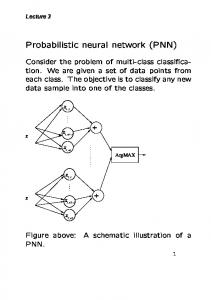
Probabilistic neural network (PNN) Consider the problem of multi-class classification. We are given a set of data points from each class. The objective is to classify any new data sample into one of the classes. x1 ,1
x
x1 ,n1−1
+
x1 ,n1
ArgMAX
x2 ,1
x
x2 ,n2−1
+
x2 ,n2
Figure above: A schematic illustration of a PNN. 1
Lecture 3
Probabilistic neural network (PNN) is closely related to Parzen window pdf estimator. A PNN consists of several sub-networks, each of which is a Parzen window pdf estimator for each of the classes. The input nodes are the set of measurements. The second layer consists of the Gaussian functions formed using the given set of data points as centers. The third layer performs an average operation of the outputs from the second layer for each class. The fourth layer performs a vote, selecting the largest value. The associated class label is then determined. 2
Lecture 3
Suppose that for class 1, there are five data points x1,1 = 2, x1,2 = 2.5, x1,3 = 3, x1,4 = 1 and x1,5 = 6. For class 2, there are 3 data points x2,1 = 6, x2,2 = 6.5, x2,3 = 7. Using the Gaussian window function with σ = 1, the Parzen pdf for class 1 and class 2 at x are y1(x) =
5 1 X
− x)2
(x1,i 1 √ exp − 5 i=1 2π 2
!
3 1 X
− x)2
!
and (x2,i 1 √ y2(x) = exp − 3 i=1 2π 2
respectively. The PNN classifies a new x by comparing the values of y1(x) and y2(x). If y1(x) > y2(x), then x is assigned to class 1; Otherwise class 2. For this example y1(3) = 0.2103 (see Lecture 2). 3
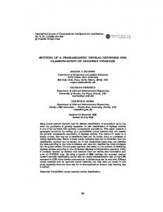
Lecture 3
0.4
0.35
0.3
0.25
y (x) 2
y (x) 1
0.2
0.15
0.1
0.05
0 −15
−10
−5
0
5
10
15
Figure above, Parzen window pdf for two classes. (
1 exp − y2(3) = √ 3 2π + exp −
(6 − 3)2 2
(6.5 − 3)2
+ exp −
2
(7 − 3)2 2
!
!
!)
= 0.0011 < 0.2103 = y1(x) so the sample x = 3 will be classified as class 1 using PNN. 4
Lecture 3
The decision boundary of the PNN is given by y1(x) = y2(x). So (
1 √ exp − 3 2π
(6 − x)2 2
+ exp − (
1 = √ exp − 5 2π + exp −
!
(7 − x)2 2
(2 − x)2 2
(3 − x)2 2
!
+ exp −
+ exp −
(6.5 − x)2
!)
+ exp −
+ exp −
(6 − x)2 2
2
!
(2.5 − x)2 2
(1 − x)2 2
!!
!
!)
The solution of x can be found numerically. e.g. a grid search. This is an optimal solution, minimizing misclassification rate. 5
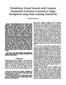
Lecture 3
Figure above: Decision boundary and the error probability of PNN (the shaded area). Moving the decision boundary to either side would increase the misclassification probability.
6
Lecture 3
Since the term √1
2π
is a common factor in both
y1(x) and y2(x), it can be dropped out without changing the classification result. We can use y1(x) = and y2(x) =
5 1 X
5 i=1 3 1 X
3 i=1
exp −
exp −
(x1,i
− x)2
!
− x)2
!
2 (x2,i
2
In general, a PNN for M classes is defined as yj (x) =
nj 1 X
nj i=1
exp −
− xk)2
(kxj,i 2σ 2
!
j = 1, ..., M where nj denotes the number of data points in class j. The PNN assigns x into class k if yk (x) > yj (x), j ∈ [1, ..., M ]. kxj,i − xk2 is calculated as the sum of squares. e.g. if xj,i = [2, 4]T , x = [3, 1]T , then kxj,i − xk2 = (2 − 3)2 + (4 − 1)2 = 10 7
Lecture 3
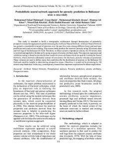
Example 1: Determine the class label for the data sample x = [0.5, 0.5]T by using a two class PNN classier, with σ = 1, based on the two class data sets given in the following Table.
x1,1 1 0 x1,2 0 1 x1,3 1 1
x2,1 -1 0 x2,2 0 -1
class 1
class 2
Solution: 1 y1(x) = {exp − 3 + exp − + exp −
(1 − 0.5)2 + (0 − 0.5)2 2
(0 − 0.5)2 + (1 − 0.5)2 2
(1 − 0.5)2 + (1 − 0.5)2 2
!
!
}
= 0.7788 8
!
Lecture 3
y2(x) =
1 {exp − 2
+ exp −
(−1 − 0.5)2 + (0 − 0.5)2 2
(0 − 0.5)2 + (−1 − 0.5)2 2
!
!
= 0.4724 Because y2(x) < y1(x), so x = [0.5, 0.5]T is classified as Class 1. 2
Class 1 Class 2 Class ?
1.5
1
0.5
0
−0.5
−1
−1.5
−2 −2
−1.5
−1
−0.5
0
0.5
1
1.5
2
Figure above, Data points in Example 1. 9