Projected free energies for polydisperse phase equilibria Peter Sollich∗ and Michael E. Cates
arXiv:cond-mat/9711312v1 [cond-mat.stat-mech] 28 Nov 1997
Department of Physics and Astronomy, University of Edinburgh, Edinburgh EH9 3JZ, U.K. A ‘polydisperse’ system has an infinite number of conserved densities. We give a rational procedure for projecting its infinite-dimensional free energy surface onto a subspace comprising a finite number of linear combinations of densities (‘moments’), in which the phase behavior is then found as usual. If the excess free energy of the system depends only on the moments used, exact cloud, shadow and spinodal curves result; two- and multi-phase regions are approximate, but refinable indefinitely by adding extra moments. The approach is computationally robust and gives new geometrical insights into the thermodynamics of polydispersity. PACS numbers: 05.20.-y, 64.10.+h, 82.70.-y, 61.25.Hq. To appear in Physical Review Letters.
struct from f [ρ(σ)] an (optimally) projected free energy surface in a reduced subspace of density variables. For these variables, we choose linear combinations of denR sities, the ‘generalized moments’ mi = dσ wi (σ)ρ(σ) of ρ(σ), defined by certain weight functions wi (σ); these are ordinary (non-normalized) moments if wi (σ) = σ i . The simplest imaginable case is where the free energy f depends only on a finite set of K such moments:
The thermodynamics of mixtures of several chemical species is, since Gibbs, a well established subject (see e.g. [1]). But many systems arising in nature and in industry contain, for practical purposes, an infinite number of distinct, though similar, chemical species. Often these can be classified by a parameter, σ, say, which could be the chain length in a polymeric system, or the particle size in a colloid; both are routinely treated as continuous variables. In other cases (see e.g. [2–5]) σ is instead a parameter distinguishing species of continuously varying chemical properties. The thermodynamics of polydispersity (thus defined) is therefore of crucial interest to wide areas of science and technology. Standard thermodynamic procedures [1] for constructing phase equilibria in a system of volume V containing M different species can be understood geometrically in terms of a free energy surface f (ρj ) (with f = F/V ) in the M -dimensional space of density variables ρj . Tangent planes to f define regions of coexistence, within which the free energy of the system is lowered by phase separation. The volumes of coexisting phases follow from the wellknown ‘lever rule’ [1]. Here ‘surface’ and ‘plane’ are used loosely, to denote manifolds of appropriate dimension. This procedure becomes unmanageable, both conceptually and numerically, in the limit (M → ∞) of a polydisperse system. There is now a separate conserved density ρ(σ) forR each value of σ; the overall density of particles is ρ = dσ ρ(σ). The free energy surface is f = f [ρ(σ)] which resides in an infinite dimensional space. Gibbs’ rule allows the coexistence of arbitrarily many thermodynamic phases. Experimentally, one often restricts attention to the cloud- and shadow-curves (also referred to as dew/bubble curves). For a fixed ‘shape’ of polydispersity ρ(σ) ˜ = ρ(σ)/ρ, these define as a function of the overall particle density ρ (and temperature T ) the onset of two-phase equilibrium (cloud-curve) and the density of the corresponding minority phase (its shadow); see e.g. [3,6,7]. Theoretical work has likewise focused on attempts to bring the problem into a more manageable form by somehow reducing its dimensionality [3–6,8–17]. In this Letter we propose a new and general method, whereby we con-
f = f (mi ),
i = 1...K
(1)
In coexisting phases one demands equality of particle chemical potentials, defined as µ(σ) = δf /δρ(σ) = P P µ w (∂f /∂m )w (σ) = i i i i i (σ), for all σ. But this i implies that all ‘moment’ chemical potentials, µi ≡ ∂f /∂mi , are likewise equal among phases. The osmotic pressures Π of all phases also mustPbe equal; simple algebra establishes that −Π = f − i µi mi which involves only the moments mi and their chemical potentials µi . Finally, if the overall σ-distribution is ρ(0) (σ), and there are p coexisting phases with σ-distributions ρ(α) (σ), each occupying a fraction φ(α) of the total volume (α = 1 . . . p), then conservation of particles implies the P usual ‘lever rule’ (or material balance) among (α) (α) ρ (σ) = ρ(0) (σ), ∀σ. Multiplying this species: αφ by a weight function wi (σ) and integrating over σ shows that the lever rule also holds for the moments: p X
(α)
φ(α) mi
(0)
= mi
(2)
α=1
These results express the fact that any linear combination of conserved densities (a generalized moment) is itself a conserved density in thermodynamics. Therefore, if the free energy of the system depends only on K moments mi . . . mK we can view these as the densities of K ‘quasispecies’ of particles, and construct the phase diagram via the usual construction of tangencies and the lever rule. Formally this has reduced the problem to finite dimensionality by a projection, although this is trivial here because f , by construction, has no dependence on any variables other than the mi (i = 1 . . . K). 1
as assumed above, f˜ = f˜(mi ) only depends on the moments retained, this amounts to maximizing the entropy in (3), while holding fixed the values of the moments mi . At this point, the factor R(σ) in (3), which is immaterial if all conservation laws are strictly obeyed, becomes central. Indeed, maximizing the entropy over all distributions ρ(σ) at fixed moments mi yields ! X λi wi (σ) (4) ρ(σ) = R(σ) exp
Of course, it is uncommon for the free energy f to obey (1). In particular, the ‘ideal gas’ (or, for polymers, Flory-Huggins) entropy term, in mixtures of many species, is definitely not of this form. On the other hand, in very many thermodynamic (especially mean field) models the free energy takes the form (kB = 1) Z ˜ f = f (mi ) + T dσ ρ(σ) [ln (ρ(σ)/R(σ)) − 1] , (3) in which the excess free energy f˜ does depend only on K moments. Examples include polydisperse hard spheres [8], polydisperse homo- and copolymers [2–5,9], and van der Waals fluids with factorized interaction parameters [10]. Note that, in the ideal gas term of (3), we have included a dimensional factor R(σ) inside the logarithm: since the resulting contribution is linear in densities, this has no effect in rigorous thermodynamics. However, it will play a central role in our approach. In principle, the phase equilibria stemming from (3) can be computed exactly by a finite algorithm. Specifically, the spinodal stability criterion involves a Kdimensional square matrix [11–14] whereas calculation of p-phase equilibrium involves solution of (p − 1)(K + 1) strongly coupled nonlinear equations. This method has certainly proved useful [2–4,9,10,14], but is cumbersome, particularly if one is interested mainly in cloud- and shadow-curves, rather than coexisting compositions deep within multi-phase regions [2,4,7,9]. Various ways of simplifying the procedure exist [6,11,15–17], but there has been, up to now, no systematic alternative to the full computation. Note also that the nonlinear phase equilibrium equations permit no simple geometrical interpretation or qualitative insight akin to the familar rules for constructing phase diagrams from the free energy surface of a finite mixture. Our method instead proceeds by deriving from (3) a ‘projected’ free energy that depends only on a finite set of moments. We argue that the most important moments to treat correctly are those that actually appear in the excess free energy f˜(mi ). Accordingly we divide the infinite-dimensional space of σ-distributions into two orthogonal subspaces: a ‘moment subspace’, which contains all the degrees of freedom of ρ(σ) that contribute to the moments mi (this subspace is spanned by the weight functions wi (σ)), and a ‘transverse subspace’ which contains all remaining degrees of freedom (as can be varied without affecting the chosen moments mi ). Physically, it is reasonable to expect that these ‘leftover’ degrees of freedom play a relatively minor role in the phase equilibria of the system, a view justified a posteriori below. Accordingly, we now allow violations of the lever rule, so long as these occur solely in the transverse space. The ‘transverse’ degrees of freedom, instead of obeying the strict particle conservation laws, are chosen so as to minimize the free energy: they are treated as ‘annealed’. If,
i
where the Lagrange multipliers λi are chosen to give ! Z X λi wi (σ) (5) mi = dσ wi (σ) R(σ) exp i
The corresponding minimum value of f then defines our projected (i.e., annealed) free energy ! X (6) λi mi − m0 fpr (mi ) = f˜ + T i
R
In the last term, m0 = dσ ρ(σ) is the ‘zeroth moment’ which is identical to the overall particle density ρ defined previously. If this is among the moments used for the projection, the resulting linear term can be dropped; otherwise it must be retained (with m0 now expressed as a function of the mi , via the λi ). Our maximum entropy method yields a free energy fpr (mi ) which only depends on the chosen set of moments: i.e., (6) is of the form (1) [18]. A finite dimensional phase diagram can now be constructed from it according to the usual rules. Obviously, though, the results now depend on R(σ) which is formally a ‘prior distribution’ for the entropy maximization. To understand its thermodynamic role, we recall that our projected free energy fpr (mi ) was constructed as the minimum of f [ρ(σ)] at fixed mi ; that is, fpr is the lower envelope of the projection of f onto the moment subspace. Crucially, the shape of this envelope depends on how, by choosing a particular prior distribution R(σ), we ‘tilt’ the infinitedimensional free energy surface before projecting it. To find the optimum choice of prior, we note that R(σ) serves physically to determine which distributions ρ(σ) lie within the maximum-entropy family (4) that the annealed system can have. Typically, one is interested in a system where a fixed overall ‘parent’ (or ‘feed’) distribution ρ(0) (σ) becomes subject to separation into various phases. In such circumstances, we should generally choose this parent distribution as our prior, R(σ) = ρ(0) (σ), thereby guaranteeing that it is contained within the family (4). Having done this, we note that the annealing procedure will be exactly valid, to whatever extent the σ-distributions actually arising in the various coexisting phases of the system under study are members of the family (4). (This statement of exactness, and similar ones below, of course hold only if (3) is valid.) 2
In fact, the condition just described does hold whenever all but one of a set of coexisting phases are of infinitesimal volume compared to the majority phase. This is because the σ-distribution, ρ(0) (σ), of the majority phase is negligibly perturbed, whereas that in each minority phase differs from this by an exponential GibbsBoltzmann factor, of exactly the form required for (4). Accordingly, our projection method yields exact cloudcurves and shadow-curves. By the same argument, critical points (which in fact lie at the intersection of these two curves) are exactly determined. Moreover, all spinodals are also found exactly by our annealing method. For, at a spinodal, there exists an instability direction (in the full space) along which the curvature of the free energy vanishes; in all other directions f has positive curvature. One can show that such an instability direction always connects neighboring distributions within the same maximum entropy family (4), and hence that only the free energy of such distributions (i.e., the projected free energy with the parental R(σ)) is needed to calculate spinodals. The geometrical interpretation of this result, and also proofs of it and the others stated above, will be given elsewhere [19]. The method does, however, give only approximate results for coexistences involving finite amounts of different phases. This is because linear combinations of different σ-distributions obeying (4), corresponding to two (or more) phases arising from the same parent (ρ(0) (σ) = R(σ)) do not necessarily add to recover the parent distribution itself. Moreover, according to Gibbs’ phase rule, a projected free energy depending on n moments will not normally predict more than n + 1 coexisting phases, whereas a polydisperse system can in principle separate into an arbitrary number of phases. Both of these shortcomings can be overcome by systematically including additional moments within the annealing procedure. (The above exact results are unaffected, because these do not exclude a null dependence of f˜ on certain of the mi .) Indeed, by adding further moments one can indefinitely expand the maximum-entropy family (4) of σ-distributions, thereby approaching with increasing precision the actual distributions in all phases present; this yields phase diagrams of ever-refined accuracy. How quickly convergence to the exact results occurs depends on the choice of weights functions for the additional moments; this will be quantified elsewhere [19]. To demonstrate the power of our approach, we consider a specific example. This is a simplified model of chemical fractionation, in which one considers species of continuously variable chemical character (such as aromaticity) governed by a parameter σ between 0 and 1. We suppose that the interaction energy between species varies as (σ − σ ′ )2 , so that the most different species repel each other most strongly. For simplicity we take a molten system, choosing volume units so that the overall density is R constrained as dσ ρ(σ) = 1. Within a mean-field treat-
50 6 40
8
3 χ
30 10/exact 4
20 2 10 0 0.1
1
0.3
0.5 m1
0.7
0.9
FIG. 1. Coexistence curves for a parent distribution with (0) m1 = 0.6. Shown are the values of m1 of the coexisting phases; horizontal lines guide the eye where new phases appear. Curves are labeled by n, the number of moments retained in the projected free energy. Predictions for n = 10 are indistinguishable from an exact calculation (in bold).
ment, the system is then described by a free energy of the form (3), with an excess free energy (in units of kB T ) R of f˜ = −χm21 , m1 = dσ σρ(σ) (up to irrelevant terms linear in ρ(σ)). This model differs only by a rescaling of parameters (with powers of polymer molecular weight) from the Flory-Huggins treatment of random AB copolymers, in which χ is the usual interaction parameter and σ is the proportion of A monomers in a chain [2–4]. The model should show fractionation into an ever-increasing number of phases as χ is increased. It is therefore an interesting test case for our projection approach (and the method of adding further moments), yet simple enough for exact phase equilibrium calculations to remain feasible, allowing detailed comparisons to be made. We consider phase separation from parent phases with σ distributions of the form ρ(σ) ∝ exp(λσ) (for 0 ≤ σ ≤ (0) 1); λ is thereby fixed in terms of the parental m1 = m1 . (0) Fig 1 shows the exact coexistence curve for m1 = 0.6, along with the predictions R from our projected free energy with n moments (mi = dσ σ i ρ(σ), i = 1 . . . n) retained. (0) Comparable results are found for other m1 . Even for the minimal set of moments (n = 1) the point where phase separation first occurs on increasing χ is predicted correctly (this is a cloud point for the given parent). As more moments are added, the annealed coexistence curves approach the exact one to higher and higher precision [20]. As expected, the precision decreases at high χ, where fractionated phases proliferate; in this region, the number of coexisting phases predicted by the projection method increases with n. However, it is not always equal to n + 1, as one might expect from a naive use of Gibbs’ phase rule; three-phase coexistence, for example, is first predicted for n = 4 [21]. Note that the stability 3
of the results to the addition of extra moments provides, in this example, a good test of convergence on the coexistence curves. For the computational implementation of both the annealing and the exact method we used a NewtonRaphson nonlinear equation solver. The annealed calculation turned out to be significantly more robust with respect to the choice of initial values, the size of χ increments etc. due to an effective decoupling of the equations: Equality of chemical potentials is achieved using the moments contained in the excess free energy, while the lever rule is satisfied (increasingly accurately) using the remaining moments [19]. This advantage should be much more pronounced in more complex cases, as should savings in computer time (which are modest in our simple example). With exact results for cloud- and shadow-curves, critical points and spinodals, as well as refinably accurate coexistence curves and multi-phase regions, our annealing method allows rapid and accurate computation of the phase behavior of many polydisperse systems. Moreover, by establishing the link to a projected free energy fpr (mi ) as a function of a finite set of conserved densities mi , it restores to the problem much of the geometrical interpretation and insight (as well as the computational methodology) associated with phase diagrams for finite mixtures. This contrasts with procedures commonly used for systems in which the excess free energy involves a finite set of moments (3) [2–5,9,10]. Some previous approximations to that problem have used (generalized) moments as coordinates; see e.g. [11,14,15,17,22]. Our annealing method provides a rational basis for these methods and, by a careful choice of prior, guarantees that many properties of interest are found exactly. Finally, our method may extend to models for which the excess free energy cannot be written directly in terms of a finite number of moments as in (3). For example, many mean-field theories correspond to a variational minimization of the free energy: F ≤ hEi0 − T S0 , where subscript 0 refers to a trial Hamiltonian [23]. In such a case, one might choose to first make a physically motivated decision about which (and how many) moments mi to keep, and then include among the variational parameters the annealed “transverse” degrees of freedom. This would lead directly to a mean-field estimate of the projected free energy without assuming Eq. (3). Note that a good choice of prior R(σ) will again be important. Although no exact results can be guaranteed, this approach may form a promising basis for future developments. Acknowledgements: After this work was substantially complete, we learned from P. B. Warren [24] that he has independently developed an approach which, though based on distinctly different principles, yields a formalism broadly equivalent to our own [19]. We thank him, and also N. Clarke, R. M. L. Evans, T. McLeish, P. Olmsted, and W. C. K. Poon, for helpful discussions.
∗
[1] [2] [3] [4] [5] [6] [7] [8] [9] [10] [11] [12]
[13] [14] [15] [16] [17] [18]
[19] [20]
[21]
[22]
[23] [24]
4
Royal Society Dorothy Hodgkin Research Fellow. Electronic address:
[email protected]. R. T. DeHoff, Thermodynamics in Material Science (McGraw-Hill, New York, 1992). B. J. Bauer, Polymer Eng. Sci. 25, 1081 (1985). M. T. R¨ atzsch and C. Wohlfarth, Adv. Polymer Sci. 98, 49 (1991). A. Nesarikar, M. Olvera de la Cruz, and B. Crist, J. Chem. Phys. 98, 7385 (1993). K. Solc, Makromol. Chem.-Macromol. Symp. 70-1, 93 (1993). P. A. Irvine and J. W. Kennedy, Macromol. 15, 473 (1982). N. Clarke, T. C. B. McLeish, and S. D. Jenkins, Macromol. 28, 4650 (1995). J. J. Salacuse and G. Stell, J. Chem. Phys. 77, 3714 (1982); L. Blum and G. Stell, ibid., 71, 42 (1979). K. Solc and R. Koningsveld, Coll. Czech. Chem. Comm. 60, 1689 (1995). J. A. Gualtieri, J. M. Kincaid, and G. Morrison, J. Chem. Phys. 77, 521 (1982). P. Irvine and M. Gordon, Proc. R. Soc. London A 375, 397 (1981). S. Beerbaum, J. Bergmann, H. Kehlen, and M. T. R¨ atzsch, Proc. R. Soc. London A 406, 63 (1986) and 414, 103 (1987). E. M. Hendriks, Ind. Eng. Chem. Res. 27, 1728 (1988). E. M. Hendriks and A. R. D. Vanbergen, Fluid Phase Eq. 74, 17 (1992). R. L. Cotterman and J. M. Prausnitz, Ind. Eng. Chem. Proc. Des. Dev. 24, 434 (1985). S. K. Shibata, S. I. Sandler, and R. A. Behrens, Chem. Eng. Sci. 42, 1977 (1987). P. Bartlett, J. Chem. Phys. 107, 188 (1997). Numerically, it is easier to view the annealed free energy as a function of the Lagrange multipliers λi rather than the moments mi , to avoid having to invert eqs. (5). M. E. Cates, P. Sollich, and P. B. Warren, in preparation. The precision of the annealed coexistence curves should depend on the total number of moments n, rather than the number of moments in the excess free energy, K. Hence the minimal annealed theory (n = K), poor for our K = 1 case, should perform better for more realistic (larger K) models. Computational effort, on the other hand, is mainly sensitive to K (the dimension of the space to be searched for new phases), rather than n. For fractionation problems such as this (but not more generally), the low temperature limit suggests that to obtain n + 1 phases, one may have to include up to 2n moments. Using localized weight functions (rather than powers of σ) for the extra moments can reduce this number, but gives less accurate coexistence curves [19]. Note also that the commonplace method of ‘binning’ the σ-distribution into discrete ‘pseudo-components’ is a special case of our annealing method in which each weight function is zero outside the corresponding bin. R. P. Feynman, Statistical Mechanics (Benjamin, Reading, MA, 1972). P. B. Warren, Phys. Rev. Lett. ??, ???? (1998).