Proofs for the Working Engineer - ETH E-Collection

DISS. ETH NO. 17671

Proofs for the Working Engineer A dissertation submitted to ETH ZURICH for the degree of Doctor of Sciences

presented by

Farhad Dinshaw Mehta Master of Science, Technische Universität M¨ unchen Bachelor of Technology, Indian Institute of Technology Delhi born 11.01.1980 citizen of India

accepted on the recommendation of Prof. Jean-Raymond Abrial Prof. Peter M¨ uller Prof. Cliff Jones

2008

Abstract Over the last couple of decades the advantages of including formal proof within the development process for computer based systems has become increasingly clear. This has lead to a plethora of logics and proof tools that propose to fulfill this need. Nevertheless, the inclusion of theorem proving within the development process, even in domains where clear benefits can be expected, is rather an exception than the rule. One of the main goals of the formal methods endeavour is to bring the activity of formal theorem proving closer to the engineer developing computer based systems. This thesis makes some important practical contributions towards realising this goal. It hopes to shows that proper tool support can not only ease theorem proving, but also strenghten its role as a design aid. It shows that it is feasible to integrate interactive proof within a reactive development environment for formal systems. It shows that it is possible to design a proof tool whose reasoning capabilities can be easily extended using external theorem provers. It proposes a representation for the proofs constructed using such an extensible proof tool, such that these proofs can be incrementally reused, refactored, and revalidated. On the more theoretical side, but with major practical implications, it shows how one can formally reason about partial functions without abandoning the well understood domain of classical two-valued predicate calculus. The ideas presented here have been used to design and implement the proof infrastructure for the RODIN platform which is an open, extensible, industry-strength formal development environment for safety critical systems. Nevertheless, the contributions made in this thesis stand on their own and are independent of the tool implementing them. This thesis is therefore not a description of a working proof tool, but the resulting tool is a proof of the feasibility of the ideas presented in this thesis.

i

ii

Zusammenfassung Das Ziel dieser Arbeit ist, dem Entwickler computergest¨ utzte formale Beweise näherzubringen. In den letzten Jahrzehnten ist mehr und mehr klar geworden, dass es vorteilhaft ist, formale Beweise in den Entwicklungsprozess von computerbasierten Systemen miteinzubeziehen. Dadurch ist eine Vielzahl von Logiken und Beweiswerkzeugen entstanden, die versprechen, diesen Ansatz in die Tat umzusetzen. Trotzdem ist es eher die Ausnahme als die Regel, dass formale Beweise in den Entwicklungsprozess miteinbezogen werden, selbst in Bereichen, in denen deutliche Gewinne erzielt werden können. Wir beginnen, indem wir versuchen, Gr¨ unde f¨ ur die langsame Akzeptanz des formalen Beweisens bei Entwicklern zu finden. Wir zeigen auf, dass praktische Anwendungen spezielle, aber u ¨berschaubare Anforderungen an Beweiswerkzeuge stellen. Damit computergest¨ utztes Beweisen industriell genutzt werden kann, m¨ ussen diese Anforderungen untersucht werden. Dies hat Konsequenzen f¨ ur das Design von Beweiswerkzeugen. Wir zeigen in dieser Arbeit, dass computergest¨ utztes Beweisen als ein ingineurswissenschaftliches Werkzeug verwendet werden kann, so dass Beweise ein praktikabler Teil des Endproduktes werden. Wir erklären dar¨ uber hinaus, wie Beweise die Entwicklung von computerbasierten Systemen unterst¨ utzen. Die hier vorgestellten Ideen sind verwendet worden, um die Beweisinfrastruktur der RODIN Plattform zu entwickeln. Die RODIN Plattform ist eine freie, erweiterbare, praxisnahe Entwicklungsumgebung f¨ ur sicherheitskritische Systeme. Dennoch sind die Beiträge dieser Arbeit unabhängig von dem Werkzeug, in dem sie umgesetzt wurden. Diese Arbeit ist daher keine Beschreibung eines Beweiswerkzeugs, jedoch ist das Werkzeug ein Beweis f¨ ur die Umsetzbarkeit der Ideen aus dieser Arbeit.

iii

iv

Acknowledgments I would like to start by thanking Prof. Jean-Raymond Abrial for being not only a patient and dedicated mentor, but also a dear friend during the three years I spent working with him. I am also very grateful to Laurent Voisin for his help with many of the ideas that have gone into this thesis. Additionally, ´ am Darvas, I would like to thank Son Thai Huang, Stefan Hallerstede, Ad´ Vijay D’silva, Achim Brucker, Burkhart Wolf and Joseph Ruskevitz for the numerous discussions I have had with them, and for making for my stay at the the ETH so enjoyable. I am grateful to Prof. Peter M¨ uller and Prof. Cliff Jones for taking the time to read and comment on my thesis. My research was funded by the EU research project IST 511599 (RODIN). I am also deeply indebted to Prof. David Basin for his support, and for welcoming me to the information security group during the last six months of my stay at the ETH. Although I started my doctoral studies at the ETH in 2004, I consider the two years I spent in the Isabelle group at the Technische Universität M¨ unchen before that to be a crucial learning experience. I would like to thank Prof. Tobias Nipkow, and my other colleagues at the time for introducing me to the world of computer aided proof. From my undergraduate years, I am grateful to Prof. Sanjiva Prasad, Prof. S. Arun Kumar and Prof. Subhashis Banerjee at the Indian Institute of Technology Delhi, and Prof. Gérard Huet at INRIA Paris-Rocquencourt for kindling in me, almost through osmosis, an interest and fascination for computer science. Last, but not least, I would like to thank Yvonne Gahler and my parents, Zarin and Dinshaw Mehta for their continual support.

v

vi

Contents 1 Introduction 1.1 Motivation . . . . . . . . . . . . . . 1.2 Formal Methods . . . . . . . . . . . 1.3 Computer Aided Proof . . . . . . . 1.4 Formal Interactive Proof . . . . . . 1.5 Non Proof-based Approaches . . . . 1.6 Problems with Existing Proof Tools 1.7 Scope of this Thesis . . . . . . . . . 1.8 Contributions and Structure . . . .

. . . . . . . .

. . . . . . . .

. . . . . . . .

2 Practical Setting 2.1 Reactive Development . . . . . . . . . . 2.2 Reactive Formal Development in RODIN 2.3 A Simple Formal Development . . . . . . 2.4 A Reactive Prover - Challenges . . . . . 2.5 Prover Requirements . . . . . . . . . . . 2.6 Related Work . . . . . . . . . . . . . . . 3 Mathematical Logic 3.1 Introduction . . . . . . . . . . 3.2 Sequent Calculus . . . . . . . 3.2.1 Sequents . . . . . . . . 3.2.2 Proof Rules . . . . . . 3.2.3 Theories . . . . . . . . 3.2.4 Proofs . . . . . . . . . 3.3 Propositional Calculus . . . . 3.3.1 Predicates . . . . . . . 3.3.2 Sequents . . . . . . . . 3.3.3 Syntax of basicPC . . 3.3.4 Proof Rule Schemas . 3.3.5 Proof Rules of basicPC vii

. . . . . . . . . . . .

. . . . . . . . . . . .

. . . . . . . . . . . .

. . . . . . . . . . . .

. . . . . . . . . . . .

. . . . . . . . . . . .

. . . . . . . .

. . . . . .

. . . . . . . . . . . .

. . . . . . . .

. . . . . .

. . . . . . . . . . . .

. . . . . . . .

. . . . . .

. . . . . . . . . . . .

. . . . . . . .

. . . . . .

. . . . . . . . . . . .

. . . . . . . .

. . . . . .

. . . . . . . . . . . .

. . . . . . . .

. . . . . .

. . . . . . . . . . . .

. . . . . . . .

. . . . . .

. . . . . . . . . . . .

. . . . . . . .

. . . . . .

. . . . . . . . . . . .

. . . . . . . .

. . . . . .

. . . . . . . . . . . .

. . . . . . . .

. . . . . .

. . . . . . . . . . . .

. . . . . . . .

. . . . . .

. . . . . . . . . . . .

. . . . . . . .

1 1 2 3 3 4 5 7 8

. . . . . .

13 13 14 15 20 20 21

. . . . . . . . . . . .

23 23 23 24 24 24 25 26 26 27 27 27 28

viii

CONTENTS

3.4

3.5

3.3.6 Derived Logical Operators 3.3.7 Reasoning . . . . . . . . . 3.3.8 Summary of PC . . . . . First-order Predicate Calculus . . 3.4.1 Expressions . . . . . . . . 3.4.2 Variables . . . . . . . . . . 3.4.3 Syntax of basicFoPCe . . 3.4.4 Proof Rules of basicFoPCe 3.4.5 Syntactic Operators . . . . 3.4.6 Derived Logical Operators 3.4.7 Summary of FoPCe . . . . Conclusion . . . . . . . . . . . . .

. . . . . . . . . . . .

. . . . . . . . . . . .

. . . . . . . . . . . .

. . . . . . . . . . . .

. . . . . . . . . . . .

. . . . . . . . . . . .

. . . . . . . . . . . .

. . . . . . . . . . . .

. . . . . . . . . . . .

. . . . . . . . . . . .

. . . . . . . . . . . .

. . . . . . . . . . . .

. . . . . . . . . . . .

. . . . . . . . . . . .

. . . . . . . . . . . .

. . . . . . . . . . . .

28 29 29 30 30 31 31 31 32 32 32 33

4 Partial Functions and Well-Definedness 4.1 Introduction . . . . . . . . . . . . . . . . 4.2 Defining Partial Functions . . . . . . . . 4.2.1 Conditional Definitions . . . . . . 4.2.2 Recursive Definitions . . . . . . . 4.2.3 A Running Example . . . . . . . 4.3 Separating WD and Validity . . . . . . . 4.4 The Well-Definedness Operator . . . . . 4.4.1 Defining D . . . . . . . . . . . . . 4.4.2 Proving properties about D . . . 4.5 Well-Definedness and Proof . . . . . . . 4.5.1 Defining D for Sequents . . . . . 4.5.2 Well-Defined Sequents . . . . . . 4.5.3 WD preserving Proof Rules . . . 4.5.4 Deriving FoPCe D . . . . . . . . . 4.5.5 Summary . . . . . . . . . . . . . 4.6 Proving WDD and ValidityD . . . . . . . 4.7 Related Work . . . . . . . . . . . . . . . 4.7.1 Comparison . . . . . . . . . . . . 4.8 Conclusion . . . . . . . . . . . . . . . . .

. . . . . . . . . . . . . . . . . . .

. . . . . . . . . . . . . . . . . . .

. . . . . . . . . . . . . . . . . . .

. . . . . . . . . . . . . . . . . . .

. . . . . . . . . . . . . . . . . . .

. . . . . . . . . . . . . . . . . . .

. . . . . . . . . . . . . . . . . . .

. . . . . . . . . . . . . . . . . . .

. . . . . . . . . . . . . . . . . . .

. . . . . . . . . . . . . . . . . . .

. . . . . . . . . . . . . . . . . . .

. . . . . . . . . . . . . . . . . . .

35 35 36 36 37 38 38 40 40 41 42 42 43 45 45 49 49 50 52 54

5 Prover Architecture and Extensibility 5.1 Introduction . . . . . . . . . . . . . . . 5.2 Prover Extensibility . . . . . . . . . . . 5.3 The Basic Prover Architecture . . . . . 5.4 Programing Notation . . . . . . . . . . 5.5 Predicates . . . . . . . . . . . . . . . . 5.6 Sequents . . . . . . . . . . . . . . . . .

. . . . . .

. . . . . .

. . . . . .

. . . . . .

. . . . . .

. . . . . .

. . . . . .

. . . . . .

. . . . . .

. . . . . .

. . . . . .

. . . . . .

55 55 56 57 58 60 60

. . . . . .

CONTENTS 5.7 5.8

5.9

5.10 5.11 5.12

ix

Proof Rules . . . . . . . . . . . . . . . . . . . Reasoners . . . . . . . . . . . . . . . . . . . . 5.8.1 Reasoner Requirements . . . . . . . . . 5.8.2 Examples of Reasoners . . . . . . . . . 5.8.3 Integrating External Theorem Provers Proof Trees . . . . . . . . . . . . . . . . . . . 5.9.1 Constraints on Proof Trees . . . . . . . 5.9.2 Operations on Proof Trees . . . . . . . 5.9.3 Example Proof Tree Construction . . . Tactics . . . . . . . . . . . . . . . . . . . . . . 5.10.1 Examples of Tactics . . . . . . . . . . Related Work . . . . . . . . . . . . . . . . . . Conclusion . . . . . . . . . . . . . . . . . . . .

6 Representing and Reusing Proofs 6.1 Introduction . . . . . . . . . . . . . . 6.2 Proof Obligation Changes . . . . . . 6.2.1 Characterising Changes . . . . 6.2.2 Reacting to Changes . . . . . 6.2.3 Requirements . . . . . . . . . 6.3 Representing Proof Attempts . . . . 6.3.1 A Running Example . . . . . 6.3.2 Recording Proofs Explicitly . 6.3.3 Recording Reasoner Calls . . 6.3.4 Recording Tactic Applications 6.3.5 Summary . . . . . . . . . . . 6.4 Proof Skeletons . . . . . . . . . . . . 6.4.1 Constructing Proof Skeletons 6.4.2 Reusing Proof Skeletons . . . 6.4.3 Proof Dependencies . . . . . . 6.4.4 Satisfying Requirements . . . 6.5 Evaluation . . . . . . . . . . . . . . . 6.5.1 Success of Proof Reuse . . . . 6.5.2 Scalability . . . . . . . . . . . 6.5.3 Improved reaction times . . . 6.6 Related Work . . . . . . . . . . . . . 6.7 Conclusion . . . . . . . . . . . . . . .

. . . . . . . . . . . . . . . . . . . . . .

. . . . . . . . . . . . . . . . . . . . . .

. . . . . . . . . . . . . . . . . . . . . .

. . . . . . . . . . . . . . . . . . . . . .

. . . . . . . . . . . . . . . . . . . . . .

. . . . . . . . . . . . .

. . . . . . . . . . . . . . . . . . . . . .

. . . . . . . . . . . . .

. . . . . . . . . . . . . . . . . . . . . .

. . . . . . . . . . . . .

. . . . . . . . . . . . . . . . . . . . . .

. . . . . . . . . . . . .

. . . . . . . . . . . . . . . . . . . . . .

. . . . . . . . . . . . .

. . . . . . . . . . . . . . . . . . . . . .

. . . . . . . . . . . . .

. . . . . . . . . . . . . . . . . . . . . .

. . . . . . . . . . . . .

. . . . . . . . . . . . . . . . . . . . . .

. . . . . . . . . . . . .

. . . . . . . . . . . . . . . . . . . . . .

. . . . . . . . . . . . .

61 63 64 64 67 68 69 70 72 74 75 79 81

. . . . . . . . . . . . . . . . . . . . . .

83 83 85 86 86 88 88 90 90 91 92 93 94 94 96 100 103 105 105 107 108 110 112

x

CONTENTS

7 Reengineering Proofs 7.1 Introduction . . . . . . . . . . . . . . . 7.2 Modifying Hypotheses . . . . . . . . . 7.3 Copying and Pasting Sub-proofs . . . . 7.4 Automatic Proof Completion . . . . . 7.5 Removing Redundant Proof Steps . . . 7.6 Inserting Steps in the Middle of Proofs 7.7 Automatically Moving Sub-proofs . . . 7.8 Related Work . . . . . . . . . . . . . . 7.9 Conclusion . . . . . . . . . . . . . . . . 8 Revalidating Proofs 8.1 Introduction . . . . . . . . . 8.2 Validation Conditions . . . . 8.3 Revalidating Rule Objects . 8.4 Revalidating Proof Skeletons 8.5 Related Work . . . . . . . . 8.6 Conclusion . . . . . . . . . . 9 Conclusion 9.1 Summary of Contributions 9.2 User Evaluation . . . . . . 9.3 Future Work . . . . . . . . 9.4 Closing Remarks . . . . .

. . . .

. . . . . .

. . . .

. . . . . .

. . . .

. . . . . .

. . . .

. . . . . .

. . . .

. . . . . .

. . . .

. . . . . .

. . . .

. . . . . . . . .

. . . . . .

. . . .

. . . . . . . . .

. . . . . .

. . . .

. . . . . . . . .

. . . . . .

. . . .

. . . . . . . . .

. . . . . .

. . . .

. . . . . . . . .

. . . . . .

. . . .

. . . . . . . . .

. . . . . .

. . . .

. . . . . . . . .

. . . . . .

. . . .

. . . . . . . . .

. . . . . .

. . . .

. . . . . . . . .

. . . . . .

. . . .

. . . . . . . . .

. . . . . .

. . . .

. . . . . . . . .

. . . . . .

. . . .

. . . . . . . . .

113 . 113 . 114 . 120 . 122 . 123 . 125 . 127 . 129 . 130

. . . . . .

133 . 133 . 134 . 135 . 136 . 137 . 138

. . . .

139 . 139 . 140 . 141 . 143

Chapter 1 Introduction The aim of this chapter is to put the relevance of this thesis in perspective with computer science in general, and with formal methods in particular. It starts by pointing out the importance and inevitability of having formal interactive proof as a part of the development process for computer based systems. It then motivates the chapters that follow by discussing the problems encountered while using existing proof tools in an engineering setting.

1.1

Motivation

In comparison with other more conventional engineering sciences, informatics is in its infancy. The modern civil or mechanical engineer has a variety of tried and tested methods, and ways of thinking about the tasks of his discipline. No construction starts before performing structural analysis, nor is any mechanical device fabricated before scrutinizing its blueprint. Such procedures which are the norm in most engineering disciplines have no counterpart in informatics. Their absence is increasingly felt whenever human or financial loss occurs as a result of computer malfunction. In the year 1994 an error in the floating point unit of the Intel Pentium processor [34] cost the company an estimated $475 million in losses. In 1996 a software error in the navigation system of the Ariane 5 launcher [11] led it to explode 40 seconds after take-off. The losses resulting from the malfunction are estimated at e850 million. Both these failures could have been prevented, given that the necessary procedures to systematically engineer and verify these systems to be correct were in place [84, 59, 54, 71]. These, and other such disasters have put pressure on informatics to develop practices to ensure error-free design and construction of computerbased systems. 1

2

1.2

CHAPTER 1. INTRODUCTION

Formal Methods

The term formal methods refers to mathematically based techniques for the specification, development and verification of software and hardware systems. Formal specification is at the heart of these techniques. A formal specification is the definition, in precise mathematical terms, of the criteria by which we can judge that the future computer based system or program is working correctly. The aim of a formal method then is to ensure that a program fulfills its formal specification. Formal methods can be classified into two broad categories based on the methodology they use: Verification In this context the program being created and its formal specification live in different worlds until the last step of the development process when the program is in its finished state. At this point it is proved that the program fulfills its formal specification. In this setting, ensuring correctness is post-facto, seen an afterthought, and decoupled from the program development process. An example of the verification of a non-trivial algorithm can be found in [66]. Correct by construction In this context a programming task begins with the creation of a formal specification. The desired computer program is then created, either mechanically or manually, with this specification in mind. This creation process may involve intermediate design phases similar to an architect systematically drawing more and more detailed blue prints until all details of the construction have been worked out. Certain mathematical properties are attributed to the intermediate designs and the created program. The created program is proved to implement its formal specification, possibly via its intermediate designs. In this setting, the proof assumes a role greater than just ensuring correctness of a system, namely that of a design aid, as discussed in §6 of [62]. This idea will be developed further in chapter 2. An example of the correct construction the same non-trivial algorithm verified in [66] can be found in [4]. Regardless of the methodology used, formal methods stress on: A formal specification defining what the program is supposed to do. An implementation aimed at realizing this specification. A proof ensuring that this is actually the case. Only in this way can we be sure that a computer program does exactly what is stated in its specification.

1.3. COMPUTER AIDED PROOF

1.3

3

Computer Aided Proof

In the last century mathematics has been introspectively concerned with the mathematical nature of its own proofs [91]. The results of this for computer science is that a computer can represent proofs as data objects, just like bank accounts or CAD designs. There even exist a number of computerbased automated and interactive proof tools. The power of using computers to create and maintain formal proofs versus doing them informally on paper is that they can be checked and operated upon mechanically, and therefore efficiently and in a less error prone way. Although it is not possible for a computer to prove any arbitrary valid theorem [48] there are classes of proofs where they perform well [88]. For the rest an interactive proof is required, where human intuition is needed to steer the proof to a good conclusion.

1.4

Formal Interactive Proof

In §1.2 we have seen that proofs play a central role in the correct construction and verification of computer-based systems. Ensuring that a program conforms to its specification cannot be done automatically per se. Since the formal specification and the properties of the created system have a precise mathematical meaning, a proof of the correctness of the system with respect to its specification can be done using mathematical logic. Mathematical logic gives us the power to make sound inferences from given assumptions using truth preserving inference rules. The term formal means that expressions are handled on the basis of their ‘form’ (i.e. syntax) by precise calculational rules, in contrast to being informally handled on the basis of their interpretation (semantics) in some application domain. Additionally, by formal proofs we mean proofs not only grounded in mathematics, but also those that can be mechanically stored and checked, in contrast to those done with pencil and paper. Assuming no-one made any mistakes, proofs done with pencil and paper would be adequate. But since the exact opposite of this assumption is the raison d’être for formal methods, we need proofs that can be mechanically checked. A computer is capable of independently and efficiently checking a mathematical proof. The combination of formal proofs with computers gives us a back door to mechanically reason about properties that would otherwise be impossible to be solved automatically. For instance the halting problem says that it is impossible for a computer program to check that another computer program terminates. But a formal proof of the termination of a program (for instance

4


by showing that there is a measure on the state of the program that always decreases) can easily be checked with the help of a computer. Even failed proof attempts are of great use since they point out bugs or oversights in the system implementation, design or specification. Nevertheless, for the engineer this translates to one extra deliverable that may well end up taking longer to produce than the actual program. This would not be a problem if all such proofs could somehow be taken care of mechanically. Unfortunately there exist theoretical results [48] showing that this is not always possible for many problems of interest to us. Even so, if our main aim is to keep an engineer’s hands away from the proving process the only avenues open to us are to: Restrict ourselves to simple properties where proofs are decidable. Restrict ourselves to small systems where automated provers have a good chance of succeeding.

The next subsection discusses alternatives to the proof-based approach that try their best to live with these restrictions.

1.5

Non Proof-based Approaches

Alternatives do exist that are not proof based. These are informally referred to as ‘push-button’ solutions. The most popular of these are model checking [32], abstract interpretation [71] and testing [29]. These methods do not require the user to prove anything. The ‘proofs’ are either simple enough to be done by brute computational force, or implicit in the system, or just absent. Without the full power of formal proof at their disposal, they pose restrictions on the systems they can treat, the properties they can verify, or their completeness: Model checking works well for simple systems with a restricted, finite state space. It is most often applied to hardware designs. For software, this approach cannot be fully decidable; it may typically fail to prove or disprove a given property. Abstract interpretation has been successfully used to automatically prove the absence of run-time errors (such as null pointer and array out of bounds exceptions) for large programs. This approach is not well suited for proving very general properties (such as functional correctness) because of the compromise that needs to be made between the precision of the analysis and its decidability.

1.6. PROBLEMS WITH EXISTING PROOF TOOLS

5

Testing is currently the most widely used method for checking the correctness of programs in industry. It does not require any notion of formal proof, but has its limitations, as expressed by Dijkstra in his famous quote [40]: “Program testing can be used to show the presence of bugs, but never to show their absence”. To summarise, each of the above three approaches, although collectively more widely used than proof-based approaches, have their limitations (such as complexity of the system being developed, the properties that can be guaranteed, and completeness) when compared to in proof-based approaches. A second point to note is that model checking, abstract interpretation, and testing are all approaches used for post-facto verification since they mostly work on the final versions of executable programs, and not intermediate models of programs that may not have any notion of execution. They therefore do not aid design as well as proofs do in the correct by construction approach discussed in §1.2. Having seen some of the current alternatives to proof-based formal development and their limitations, in the rest of this thesis we will focus on easing proof-based formal development for applications where this is seen as desirable.

1.6

Problems with Existing Proof Tools

Constructing formal proofs is hard and tedious work, and typically accounts for a very large share of the total time spent doing formal development. Although a central part of this process, doing formal proof is often regarded as drudgery; something that has to be done quickly and gotten out of the way. So great is the aversion to it, that the techniques that have caught the attention of industry have largely been the ‘push-button’ solutions talked about in §1.5. In that section we have also seen that interactive formal proof is something that often becomes a necessity. The studies presented in [5], and [16] show that performing formal proofs can even be a more economical alternative to the heavy testing currently required for safety critical systems. We will therefore have to deal with the problems associated with the widespread use of formal proof tools sooner or later. In the rest of this section we give an overview of the problems, encountered when doing formal interactive proof in the engineering setting, that will be addressed in this thesis. a. Complicated Mathematical Language Although most software engineers have a knowledge of mathematics, they still need to learn how

6

CHAPTER 1. INTRODUCTION to carry out formal proof. Most of their notions of proof correspond to informal ones in mathematics. Engineers are not used to thinking of proof as a way of reasoning about and developing computer-based systems. Additionally, there exists a plethora of different logics, each with their own peculiarities and notations, which makes for a great deal of confusion.

b. Nature of Arising Proof Obligations Proof obligations arising from engineering applications are different from those that are encountered in mathematics. A medium sized formal development typically results in the generation of hundreds of proof obligations. Each of these proof obligations in turn typically contain hundreds of hypotheses, and large goals. Although most of these proof obligations are typically trivial, manually proving or even inspecting each generated proof obligations is not feasible. c. Inadequate Support for Intuitive User Interaction Although ideal user interfaces for interactive proof are an area of research in themselves [13] and will not be dealt with in this thesis, the architecture of the underlying proof tool can severely restrict the types of features that can be offered by its user interface. For instance, a user would typically like to visualise and move freely between the steps of a proof without having to undo and redo his proof. This is not possible in most proof tools since they only keep a record of the pending sub goals of a proof, and not of each proof step. d. Inadequate Support for Incremental Development The development of large computer-based systems is an incremental activity. The final product is the result of adding details and removing errors in existing designs. Changes in the development, no matter how small, are often reflected as changes in a large number proof obligations arising from it, invalidating existing proofs. Not managing such changes properly results in repetition of work and waste of previous proof effort. e. Inadequate Support for Integrating Existing Provers There exist a large number of powerful automated theorem provers that could be used to automatically discharge pending sub goals in an interactive proof and save the user from having to prove them manually. Extending the reasoning capabilities of existing proof tools using external automated theorem provers is not straightforward. A major reason for this difficulty is that proof tools are often designed as closed systems, leaving such extensions as afterthoughts.

1.7. SCOPE OF THIS THESIS

7

In §1.8 we present overview of how we propose to tackle these problems later in this thesis. Before that we first discuss the nature and scope of this thesis in the next section.

1.7

Scope of this Thesis

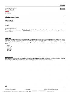
The subjects covered by this thesis lie in the intersection of the three fields of formal methods, logic, and software engineering, as illustrated in figure 1.1.

Formal Methods

Logic

Software Engineering

Figure 1.1: Scope of this Thesis. The primary contribution of this thesis is to use existing theoretical results as a basis to solve practical engineering problems. This point can be seen in analogy with the first theses in the area of compiler design. Their basis was theoretical. They depended on existing theoretical results in lexical analysis, parsing, machine grammars, etc. ,but their contribution was to solve a practical engineering problem: How to design compilers that can be used in a practical setting. In a forward to a recent book on program verification [22], K. Rustan M. Leino also touches on this point: . . . Yet, program verification tools have not reached the same kind of maturity as, say, compilers. It took many years of developing and refining the theory underlying modern compilers, including context-free grammars and data-flow analyses, but these are now taught in undergraduate computer science curricula. We can only hope that program verifiers will eventually become as well understood.

8

CHAPTER 1. INTRODUCTION . . . The ultimate goal of program verification is not the theory behind the tools, or the tools themselves, but the application of the theory and tools in the software engineering process.

As an engineering thesis, the four essential questions I try to answer are: 1. What is the engineering problem to be solved? 2. In what sense are previous solutions to this problem unsatisfactory? 3. What is my solution? 4. What evidence is there that my solution is an improvement over previous solutions? The ideas presented here have been used to design and implement the proof infrastructure for the RODIN formal development environment which is described in §2. Nevertheless, the contributions made in this thesis stand on their own and are independent of the tool implementing them. This thesis is therefore not a description of a working proof tool, but the resulting tool is a proof of the feasibility of the ideas presented in this thesis. The RODIN platform was developed by the formal methods technology group headed by Jean-Raymond Abrial at the ETH Zurich. Apart from myself, this group consisted of Laurent Voisin, Son Thai Hoang, Stefan Hallerstede and Fran¸cios Terrier. Although the development of this tool was a group effort, I have only included ideas that I have personally worked on and implemented in this thesis and have tried my best to present them independently of the RODIN tool. These ideas have been improved through discussion with my colleagues (in particular Jean-Raymond Abrial and Laurent Voisin) to whom I am grateful. The next section gives an overview of the structure and contributions of this thesis.

1.8

Contributions and Structure

The first two chapters of this thesis are motivational. They provide an overview of the setting and of the problems tackled in this thesis. Chapter 2 describes the practical setting of the work done in this thesis. Chapter 3 defines its theoretical point of departure. Chapter 4 is the major theoretical contribution of this thesis: How can one formally reason about partial functions without abandoning the well understood domain of classical two-valued predicate calculus. The remainder of the chapters are about contributions of

1.8. CONTRIBUTIONS AND STRUCTURE

9

a more engineering nature. They propose practical solutions to the following questions related to providing proof support in a tool: How can a proof tool be designed so that its reasoning capabilities are easily extensible? (chapter 5) How should proofs be stored so that they can be reused efficiently? (chapter 6) How can proofs themselves be manipulated in useful ways?(chapter 7) How can stored proofs be re-validated? (chapter 8)

Chapter 9 summarizes the main contributions of this thesis and compares its results with related approaches. Here are more detailed descriptions for each chapter: Chapter 2: Practical Setting In this chapter we describe the practical setting of the work done in this thesis. We show how the activities of modeling and proving go hand in hand, emphasising the role of proving as a modeling aid. We then talk about the tool support required to facilitate such a style of development in practice. We argue for a reactive development environment, where proofs are automatically updated whenever models change. We discuss the challenges of providing tool support for proof in such a reactive development environment. We conclude with a set of requirements for a proof tool that we use to guide its design in chapters 5 and 6. Chapter 3: Mathematical Logic In this chapter we give an overview of the mathematical notation and logic used in this thesis. We start with an abstract view of proofs in sequent calculus. We then refine this view for proofs in propositional calculus and further refine this to first-order predicate calculus with equality. The mathematical logic and notion of proof presented in this chapter will be used as the basis of discussions in the rest of the thesis. Chapter 4: Partial Functions and Well Definedness In this chapter we show how to formally reason about partial functions without abandoning the well understood domain of classical two-valued predicate calculus. In order to achieve this, we further extend our mathematical logic with the notion of well-definedness. We show how well-definedness can be used to filter out potentially ill-defined statements from proofs. We extend our existing proof calculus with a new set of derived proof rules

10

CHAPTER 1. INTRODUCTION that can be used to preserve well-definedness in order to make proofs involving partial functions less tedious to perform.

Chapter 5: Prover Architecture and Extensibility In this chapter we present the basic architecture of the proof tool and the ways in which its proving capabilities can be extended. For clarity we restrict this basic architecture to the propositional subset of our mathematical language. We show how proofs can be constructed in the proof tool, and how these constructed proofs correspond to our mathematical notion of proof discussed in chapter 3. The implementation of the proof tool is sketched using an object-oriented pseudo-code notation. This chapter provides a concrete basis for the discussions in chapters 6, 7, and 8. Chapter 6: Representing and Reusing Proofs This chapter is concerned with representing and reusing proofs constructed in the proof tool. We start by discussing the most frequently occurring proof obligation changes that we experience during reactive formal development, as discussed in chapter 2, and propose a strategy to manage such changes. We then state some concrete requirements on the way proof attempts are represented and reused. We discuss the various possibilities we have of representing proofs, and their consequences on proof reuse. We then use the requirements stated earlier to propose a new a way of representing proof attempts (that we call proof skeletons) that are resilient to change and amenable to reuse. Experimental evidence on the effectiveness of our solution to represent and reuse proofs is also presented. Chapter 7: Reengineering Proofs This chapter builds on the idea that proofs are themselves formal objects that can be manipulated to perform some useful operations. This chapter is not meant to be a catalogue of all possible proof manipulations, but uses examples to sketch some proof manipulations that are useful in an engineering setting. Chapter 8: Revalidating Proofs In this chapter we show how proof skeletons can be revalidated. In particular we show how the proof checking paradigm can be used to cross-check each step of a proof with respect to an independent third-party proof tool. Chapter 9: Conclusion This chapter brings this thesis to a close by summarizing its main contributions, providing evidence that suggests that these contributions lead to an increase in user productivity, and discussing areas of further work.

1.8. CONTRIBUTIONS AND STRUCTURE

11

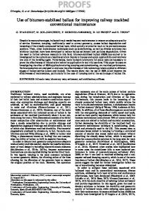
Since this thesis covers a number of subjects, figure 1.2 has been included to aid its reading. It illustrates the dependencies between the chapters of this thesis. Chapter 1

Introduction

Chapter 3

Chapter 2

Mathematical Logic

Practical Setting

Chapter 5

Prover Architecture and Extensibility

Chapter 4

Chapter 6

Partial Functions and Well-Definedness

Representing and Reusing Proofs

Chapter 7

Chapter 8

Reengineering Proofs

Revalidating Proofs

Chapter 9

Conclusion

Figure 1.2: Dependencies between the chapters of this thesis.

12


Chapter 2 Practical Setting In this chapter we describe the practical setting of the work done in this thesis. We show how the activities of modeling and proving go hand in hand, emphasising the role of proving as a modeling aid. We then talk about the tool support required to facilitate such a style of development in practice. We argue for a reactive development environment, where proofs are automatically updated whenever models change. We discuss the challenges of providing tool support for proof in such a reactive development environment. We conclude with a set of requirements for a proof tool that we use to guide its design in chapters 5 and 6.

2.1

Reactive Development

One of the major issues of software engineering is the inevitability of change. Change can occur as the result of a change in requirements, the need for new functionality, the discovery of bugs, etc. But these are not the only sources of change. Smaller incremental changes are unavoidable when developing large, real world systems. The construction of such systems is an incremental activity since, in practice, getting things right the first time around is highly unlikely [21]. Modern development environments, such as the Eclipse IDE for Java [41], support incremental construction by managing change and giving the engineer quick feedback on the consequences of the latest modification of a program. Such development tools work behind the scenes to report compile time errors while the programmer modifies his program. This quick feedback allows the programmer to immediately correct any errors while he is editing his program without having to wait till the next compile cycle, thus increasing productivity. Formal model development is also an incremental activity [85]. One of 13

14

CHAPTER 2. PRACTICAL SETTING

the major criticisms of using formal methods in practice is the lack of adequate tool support, especially for proof. The RODIN platform [1] addresses this by providing a similar reactive development environment for the correct construction of complex systems using refinement and proof. It is based on the Event-B [6] formal method. The development process consists of modeling the desired system and proving proof obligations arising from it. A proof obligation is a logical statement derived from a model. It must be proved in order to guarantee that the model is intrinsically consistent and that it refines its abstraction (if any). In the correct by construction setting introduced in §1.2, the proving process is seen as not merely justifying that certain properties of the system hold, but also as a modeling aid to help steer the course of the modeling process. In contrast to post-construction verification, the proving process assists modeling, in the same way testing and debugging assists programing. Figure 2.1 illustrates this analogue between programing and debugging, and modeling and proving. Programing

Debugging / Testing

Modeling

Proving

Figure 2.1: Programing vs Model Development

But the way the proving process is supported by formal development tools used today does not take advantage of this interaction between modeling and proving. The main reason for this is that modeling and proving are treated as isolated activities, making it hard for the user to move freely between them in order to use proving insights to aid modeling.

2.2

Reactive Formal Development in RODIN

From the experience of how a previous generation of development tools [33, 8] were used, the RODIN platform proposes a reactive development environment, similar to a modern IDE, where the user working on a model is constantly notified on the status of his proofs. To achieve this, the tools present in the RODIN platform are run in a reactive manner. This means that when a model is modified, it is automatically:

2.3. A SIMPLE FORMAL DEVELOPMENT

15

Modeling

Proving Proving UI

Error Messages

Modeling UI

Static Checker

Unchecked Model

Proof Obl. Generator

Checked Model

PO Manager & Prover

Proof Obligations

Proof Attempts & Status

Figure 2.2: The RODIN Tool Chain

1. Checked for syntax and type errors, 2. its proof obligations are generated, and 3. the status of its proofs are updated, possibly by calling automated provers, or reusing old proof attempts.

The RODIN tool chain is illustrated in figure 2.2. The user gets immediate notification on how his last modeling change affects his proofs. Inspecting failed proofs often gives the user a clue on how to further modify his model. The user may then use this feedback to make further modifications to his model, or decide to work interactively on a proof that the prover was unable to discharge automatically. A detailed description of the RODIN tools and user interface can be found in [7].

2.3

A Simple Formal Development

In this section we demonstrate the use of the RODIN reactive development environment using a simple formal development with screen-shots taken from the tool. Our aim is to show in practice how the proving process can be an aid to modeling when both these processes are tightly integrated within a reactive development environment. The user wants to model a simple bank account with operations to deposit and withdraw money from this account. The following screen-shot shows our point of departure for this simple model.

16


The user has modeled a machine called ‘Account’ with only one variable called ‘balance’ which can be incremented or decremented by a value ‘amount’ using the events ‘deposit’ and ‘withdrawal’ respectively. The invariant ‘inv1’ for this machine states that ‘balance’ is a natural number, and therefore cannot be negative. After saving this model, the tool automatically generates its proof obligations and runs a collection of automated provers on the generated proof obligations as discussed in §2.2. The tool communicates its progress in proving each proof obligation via the ‘Obligation Explorer’ as follows.


17

The tool has generated three proof obligations for this model. The first two proof obligations have √ been successfully proved automatically. This is indicated by the green ‘ ’ icon with the super-scripted ‘A’. The last proof obligation is still pending, indicated by the red ‘?’ icon. This indicates to the user that this proof obligation could not be automatically discharged. The reason for this could be either that: 1. The proof obligation is provable, but needs an interactive proof. 2. The proof obligation is not provable due to an error in the model. In order to figure out which of the above is the case, the user inspects the pending proof obligation which is then displayed to him as follows.

18


Upon inspecting this proof obligation, the user infers that it cannot be proved. This indicates that he needs to change his initial model. He then asks the tool to show him the relevant parts of the model used to generate this proof obligations in order to help him decide what to change. He is then presented with the following ‘Proof Information’.

From the above information he can clearly see that the cause of the error is that the ‘withdrawal’ event could result in a negative ‘balance’, which would invalidate the invariant ‘inv1’. He also finds two alternatives to fix this error. He could either weaken the invariant ‘inv1’ to allow ‘balance’ to have negative values, or he could add a second guard to the ‘withdrawal’ event to prevent the resulting ‘balance’ from becoming negative. He chooses the latter solution and adds a new guard ‘grd2’ to the ‘withdrawal’ event. What follows is a screen-shot of the modified model, with the added guard highlighted in blue:


19

Upon saving this modified model, the tool runs in the background to recompute the status of its proof obligations and updates them as follows:

20


The user now sees that all three proof obligations have been proved and can continue with his development. The tool did not need to re-run the automated provers on the first two proof obligations that were previously discharged, but only on the third proof obligation that was modified as a result of the modeling change. Supporting such a reactive development environment poses new challenges for the tools involved, particularly the prover. This is the subject of the next section.

2.4

A Reactive Prover - Challenges

In a reactive development environment, a change in a model is immediately reflected as changes in proof obligations. The main challenge for a proof tool in such an environment is to make the best use of previous proof attempts in the midst of changing proof obligations. Reusing previous proof attempts is important since considerable computational and manual effort is needed to produce a proof. This problem will be tackled in chapter 6 of this thesis.

2.5

Prover Requirements

It is our view that the major bottleneck in doing formal development is the time and effort required for proof. We conclude this chapter with two highlevel requirements for the proof tool used in the RODIN platform that we treat in this thesis that address this bottleneck: Efficiency We require that the proof tool runs efficiently so that the user can be provided with instant feedback of the effect of his modeling changes on his proofs. The proof tool must therefore be aware of changes and

2.6. RELATED WORK

21

be able to efficiently recover from them. This requirement heavily influences the way proof attempts are represented and reused in chapter 6. Extensibility Since it is hard to anticipate the types of proof obligations that the user may encounter in the future, we additionally require that the reasoning capabilities of the proof tool are easily extensible. This requirement heavily influences the architecture of the proof tool in chapter 5.

2.6

Related Work

Reactive development environments for program development such as Eclipse [41] have been around for some time now, and have significantly increased the productivity of software engineers by integrating development tools such as compilers, debuggers and program analysers to avoid having developers call these tool individually. In this section we present related work in the area of development environments that support formal proof. The idea of generating proof obligations (or verification conditions) from program texts has been around since James King’s 1970 thesis [60] and has been used in a large number of verification approaches, the most recent of which include VDM [56], KIV [15], Jive [69], KeY [22], Isabelle/HOL/Hoare [72], ESC/Java [64], Caduceus [43], JACK [20] and Spec# [18], just to name a few. But, with the exception of the Boogie program verifier [17] treated in the next paragraph, none of the currently used formal development tools support the type of direct modelingproving interaction that we have demonstrated in this chapter. Moving between the modeling and proving activities in such development tools requires explicit manual interaction to check models, generate proof obligations, and reload proofs. This increases the time required to switch between modeling and proving and reduces the impact of proving as a modeling aid. The Boogie program verifier [17] is integrated within the Visual Studio development environment for C#. It accepts program specifications as assertions in Spec# and provides ‘design-time feedback’ of possibly invalid assertions to the programmer. A central design decision of Boogie is that it only uses automated provers to check the validity of the verification conditions it generates. The main difference between the Boogie approach and the one taken in the RODIN platform is that the latter approach also supports interactive proof, which gives the user an extra degree of freedom since he is not restricted to only entering models that can be automatically proved,

22


but may additionally decide to interactively prove proof obligations that are valid, but not automatically provable. To provide this extra freedom, the RODIN platform needs to additionally manage additional user input in the form of interactive proof attempts. Chapter 6 describes how this is done. Extending Boogie to support interactive proof can also be done along similar lines.

Chapter 3 Mathematical Logic In this chapter we give an overview of the mathematical notation used in this thesis. The mathematical logic and notion of proof presented in this chapter will be used as the basis of discussions in the chapters to come.

3.1

Introduction

The mathematical notion of proof plays a central role in this thesis. This notion of proof will be used in two ways: 1. It is used to perform actual proofs in chapters 4 and 8. 2. It is used as a specification for proofs generated using the proof tool introduced in chapter 5. The aim of this chapter is to formally define what we mean by a mathematical proof. We start with an abstract view of proofs in sequent calculus in §3.2. We then refine this view for proofs in propositional calculus in §3.3 and further refine this to first-order predicate calculus with equality in §3.4. The logic is developed in a style similar to the one used in [3] and [6] to develop the logic used for the B and Event-B methods. Although some of the individual proof rules have been modified to conform more closely to those from the (single succedent) sequent calculus [47], both sets of rules are equivalent.

3.2

Sequent Calculus

In this section we present an abstract view of proofs in sequent calculus. 23

24

3.2.1

CHAPTER 3. MATHEMATICAL LOGIC

Sequents

A sequent is a generic name for a statement that we want to prove. A proof is associated with a sequent. We will refine our notion of what a sequent is in §3.3.2. In this section will use identifiers such as S1 , S2 , etc. to denote sequents. Definition 3.1 (Sequent). A sequent is a generic name for a statement that we want to prove.

3.2.2

Proof Rules

A proof rule is device used to construct proofs of sequents. It is made up of two parts, the antecedent part, and a consequent part. The antecedent part consists of a list (i.e. a finite, ordered sequence) of sequents (the antecedents). The consequent part consists of a single sequent (the consequent). The proof ~ and consequent C is written as: rule named r with antecedents A ~ A r C The proof rule r yields a proof of the sequent C as soon as we have proofs ~ The ‘~ ’ above A indicates that the antecedents are lists of each sequent in A. ~ is transformed of sequents. Using this rule, proofs of each of the sequents in A into a proof of C. Alternatively, if we want to prove C, after applying the ~ rule r to it we only need to prove the sequents in A. Definition 3.2 (Proof Rule). A proof rule is a device used to construct proofs of sequents. It consists of a list of antecedent sequents, and a consequent sequent. ~ is empty, the rule is said to discharge the In case the list of antecedents A sequent C. Here are some examples of proof rules: S2

3.2.3

S3 S1

S4

r1

S5 S2

S6 r2

S7 r3 S3

S4

r4

Theories

A theory or calculus is a set of proof rules. This set is normally infinite and is specified using a finite set of proof rule schemas. At the moment we do not have enough logical machinery to show how this takes place. We will come back to this point later in §3.3.4.

3.2. SEQUENT CALCULUS

25

Definition 3.3 (Theory). A theory is a (possibly infinite) set of proof rules. Here is a theory T with seven proof rules : S2

S4

3.2.4

S3 S1

S4

r4

S5

r1

S5

S2 r5

S7 r3 S3

S6 r2

S6

r6

S7

r7

Proofs

A proof is a device for combining individual proof rules to form larger inference steps. It is defined formally as follows. Definition 3.4 (Proof). A proof of a sequent within a given theory is a finite tree whose nodes have the following properties: Each node consists of a sequent and an optional proof rule of the theory. The root node contains the sequent we want to prove. A node with no proof rule has no child nodes. In case a node contains a proof rule:

– Its sequent is identical to the consequent of the proof rule. – It has a child node corresponding to each antecedent of the proof rule. – The sequent of each child node is identical to its corresponding antecedent. Here is a proof of the sequent S1 using the theory T just presented: S5

r5 S2

r6 S6 r2

S7 r3 S3 S1

S4

r4 r1

The sequent S7 is said to be a pending sub-goal of the above proof. Definition 3.5 (Pending Sub-goals of a Proof). The leaf nodes of a proof that do not contain proof rules are said to be pending nodes. The sequents of such pending nodes are said to be the pending sub-goals of a proof.

26


A proof can either be complete or incomplete. These terms are defined formally as follows. Definition 3.6 (Complete Proof). A proof is said to be complete iff it has no pending sub-goals. Definition 3.7 (Incomplete Proof). A proof is said to be incomplete iff it has at least one pending sub-goal. The proof just presented above is an example of an incomplete proof. It can be made complete by applying the rule r7 to the pending node with sequent S7 . The resulting complete proof is: S5

r5 S2

r7 S7 r3 S3

r6 S6 r2 S1

S4

r4 r1

In the next section we refine this abstract view of proofs to proofs in propositional calculus.

3.3

Propositional Calculus

In this section we define the mathematical language of propositional calculus (PC ).

3.3.1

Predicates

A predicate is a syntactic construct appearing in sequents. They are used to formally express properties that we would like to reason about using proof. Semantically, predicates can be thought of as entities having a truth value associated to them (i.e. they can either be true or false). Definition 3.8 (Predicate). A predicate is a formal statement expressing a certain property that we may assume, or a certain property that we wish to prove. Here is an example of a predicate: A∧B⇒B∧A The syntax for predicates will be defined in §3.3.3 and §3.3.6.

3.3. PROPOSITIONAL CALCULUS

3.3.2

27

Sequents

We now refine our concept of sequents introduced in §3.2.1. A sequent is composed of a finite set of hypotheses predicates, and a single goal predicate. A sequent with the hypotheses ‘H’ and the goal ‘G’ is written: H`G and is to be read as “Under the hypotheses H, prove the goal G ”. Definition 3.9 (Sequent in Predicate Calculus). A sequent in predicate calculus is composed of a finite set of hypotheses predicates ‘H’, and a single goal predicate ‘G’, written ‘ H ` G ’. We now introduce the syntax and proof rules of PC . This will be done in two steps. In the first step we introduce basicPC in §3.3.3 with a minimal syntax. In §3.3.6 we then introduce the additional derived logical operators in terms of the predicates of basicPC .

3.3.3

Syntax of basicPC

The syntax for predicates of basicPC is defined as follows: P

::=

⊥ | ¬P

| P ∧P

where ‘⊥’ is the ‘false’ predicate, and ‘¬’, ‘∧’ are the logical operators for negation and conjunction respectively.

3.3.4

Proof Rule Schemas

A theory is specified using a finite set of proof rule schemas. Each proof rule schema represents an infinite number of proof rules of the same form. A proof rules may be derived from its rule schemas by instantiating its so-called meta variables. For instance consider the rule schema: H ` P H, P ` Q cut H`Q The letters H, P , and Q are meta variables. The letter H is a meta variable standing for a finite set of predicates, whereas the letters P and Q are meta variables standing for single predicates. Replacing these meta variables by actual predicates gives us a proof rule. Here is an instance of the above rule schema:

28

CHAPTER 3. MATHEMATICAL LOGIC A ` B A, B ` C cut instantiated A`C

where A, B, and C are concrete predicates. A single proof rule schema therefore denotes an infinite number of proof rules present in a theory.

3.3.5

Proof Rules of basicPC

The proof rules of basicPC are defined using the following rule schemas: H, P ` P

hyp

H, P ` Q cut H`Q

⊥hyp

H, ¬P ` ⊥ contr H`P

H, P ` ⊥ ¬goal H ` ¬P

H ` P ¬hyp H, ¬P ` Q

H, ⊥ ` P

H`P H`Q ∧goal H`P ∧Q

3.3.6

H`P

H`Q mon H, P ` Q

H, P, Q ` R ∧hyp H, P ∧ Q ` R

Derived Logical Operators

We extend the basicPC to PC by introducing the ‘true’ predicate ‘>’, and the logical operators ‘∨’, ‘⇒’, and ‘⇔’ using the following syntactic definitions: > P ∨Q P ⇒Q P ⇔Q

= b = b = b = b

¬⊥ ¬(¬P ∧ ¬Q) ¬P ∨ Q (P ⇒ Q) ∧ (Q ⇒ P )

(3.1) (3.2) (3.3) (3.4)

Note that the ‘=’ b symbol used above represents syntactic equivalence. It is not itself part of the syntax, but a meta-logical connective. The following proof rule schemas can be derived from the above definitions and the rule schemas of basicPC from §3.3.5: H`> H ` P ∨goal 1 H`P ∨Q

>goal

H`Q ∨goal 2 H`P ∨Q

H, P ` R H, Q ` R ∨hyp H, P ∨ Q ` R

3.3. PROPOSITIONAL CALCULUS H, P ` Q ⇒goal H`P ⇒Q

29

H`P H, Q ` R ⇒hyp H, P ⇒ Q ` R

H`P ⇒Q H`Q⇒P ⇔goal H`P ⇔Q

H, P ⇒ Q, Q ⇒ P ` R ⇔hyp H, P ⇔ Q ` R

The next sub-section is a short note on the types of reasoning required in order to prove the derived rule schemas just presented, and others that appear in this thesis.

3.3.7

Reasoning

There are two forms of reasoning that we use in this thesis. The first is syntactic rewriting using syntactic definitions such as ‘> = b ¬⊥’, where all occurrences of ‘>’ in a formula may be replaced with ‘¬⊥’, purely on the syntactic level, to get a syntactically equivalent formula. The second is logical validity where we additionally appeal to the notion of proof. Most proofs done in this thesis rely on both syntactic and logical reasoning. As an example, here is a proof of the derived rule schema >goal . The derived rule appears boxed on the right, followed by its proof: H`>

>goal

⊥hyp H, ⊥ ` ⊥ ¬goal H ` ¬⊥ (3.1) H`> The first step of this proof, labelled (3.1), has been justified using the referred syntactic definition ‘> = b ¬⊥’, and the next two steps have been justified using rule schemas appearing in §3.3.5. In the proofs presented in the rest of this thesis only important proof steps are shown. Combined proof steps are justified using a sequence of previously appearing proof rules, definitions and equivalences.

3.3.8

Summary of PC

To summarise this section, here is the syntax and proof rule schemas for PC . We will later also refer to PC as the propositional subset of our mathematical language. P

::=

⊥ | > | ¬P

| P ∧P

| P ∨P

| P ⇒P

| P ⇔P

30


H, P ` P

H, ⊥ ` P

⊥hyp

H`>

>goal

H, P ` ⊥ ¬goal H ` ¬P

H, P ` R H, Q ` R ∨hyp H, P ∨ Q ` R

H`P H, Q ` R ⇒hyp H, P ⇒ Q ` R

H`P ⇒Q H`Q⇒P ⇔goal H`P ⇔Q

3.4

H, ¬P ` ⊥ contr H`P

H, P, Q ` R ∧hyp H, P ∧ Q ` R

H`Q ∨goal 2 H`P ∨Q

H, P ` Q ⇒goal H`P ⇒Q

H, P ` Q cut H`Q

H ` P ¬hyp H, ¬P ` Q

H`P H`Q ∧goal H`P ∧Q H ` P ∨goal 1 H`P ∨Q

H`P

H`Q mon H, P ` Q

hyp

H, P ⇒ Q, Q ⇒ P ` R ⇔hyp H, P ⇔ Q ` R

First-order Predicate Calculus

In this section we will refine PC with additional syntax and proof rules to obtain the first-order predicate calculus with equality (FoPCe). The syntax of PC is extended with new kinds of predicates, and also with two new syntactic categories for expressions and variables.

3.4.1

Expressions

An expression is a syntactic construct that denotes a mathematical object, such as a number, a set, a function, etc. . Definition 3.10 (Expression). An expression is a formal statement denoting a mathematical object. Here are some examples of expressions: f (x) x g(x, f (x)) The syntax for expressions will be defined in §3.4.3. An important distinction between expressions and predicates is that there is no concept of proof for an expression, as there is for predicates. One cannot prove an expression.

3.4. FIRST-ORDER PREDICATE CALCULUS

3.4.2

31

Variables

A variable is an identifier that denotes an unknown mathematical object. A variable is therefore an expression. A variable is subject to substitution (i.e. being replaced by another expression). Definition 3.11 (Variable). A variable is an identifier that denotes an unknown expression. The identifier ‘x’ is a variable in the expression ‘f (x)’ and in the predicate ‘x = f (x)’ . A predicate may contain occurrences of so called free variables. Semantically, the truth value of a predicate depends on the free variables occurring in it. We now introduce the syntax and proof rules of FoPCe. As done for PC , this will be also be done in two steps. In the first step we introduce the minimal basicFoPCe in §3.4.3 and later define additional derived logical operators in §3.4.6.

3.4.3

Syntax of basicFoPCe

Formulæ in basicFoPCe can either be predicates (P ) or expressions (E). The syntax of basicFoPCe is the syntax of basicPC extended as follows: P

::=

E

::=

| ∀x.P ~ x | f (E)

...

| E=E

~ | R(E)

~ is a list of expressions, R is a relational predicate where x is a variable, E ~ is the relational symbol, and f is a function symbol. The predicate R(E) ~ Equality is denoted by the predicate symbol R, applied to the arguments E. ~ denotes infix binary relational predicate symbol ‘=’. The expression f (E) ~ the function symbol f , applied to the arguments E.

3.4.4

Proof Rules of basicFoPCe

We add the following rule schemas to the rule schemas of basicPC to get the rule schemas for basicFoPCe: H`P ˆ H) ∀goal (x nfin H ` ∀x·P

HÈ=E

= goal

H, [x := E]P ` Q ∀hyp H, ∀x·P ` Q

H ` [x := E]P = hyp H, E = F ` [x := F ]P

32


ˆ and ‘[x := E]’ occurring in the above rule The syntactic operators ‘ nfin’ schemas are described in the next sub-section.

3.4.5

Syntactic Operators

The rules of basicFoPCe contain occurrences of so-called syntactic operators for substitution and non-freeness. The predicate ‘[x := E]P ’ denotes the syntactic operator for substitution [x := E], applied to the predicate P . The resulting predicate is P , with all free occurrences of the variable x replaced ˆ H)’ asserts that the variable by the expression E. The side condition ‘(x nfin ‘x’ is not free in any of the predicates contained in ‘H’. Both these syntactic operators are defined at the meta-logical level (using ‘=’) b on the inductive structure of the formulæ of basicFoPCe in such a way that they can always be evaluated away. Their formal definitions can be found in [6]. Syntactic operators can be thought of as ‘macros’ whose repeated replacement always results in a formula of basicFoPCe. Our basic syntax for formulæ therefore does not need to be extended to take syntactic operators into account.

3.4.6

Derived Logical Operators

To obtain the mathematical language FoPCe from basicFoPCe , we add the derived logical operators of PC , as described in §3.3.6, and the existential quantifier ‘∃’ which is defined using the following syntactic definition: ∃x·P = b ¬∀x·¬P

(3.5)

The following proof rule schemas can be derived from the above definition and the rule schemas of PC in §3.3.8 and basicFoPCe in §3.4.4: H ` [x := E]P ∃goal H ` ∃x·P

3.4.7

H, P ` Q ˆ ∃hyp (x nfinH ∪ {Q}) H, ∃x·P ` Q

Summary of FoPCe

To summarise this section, here are the additional syntactic constructs and proof rule schemas that we have added to PC (whose summary appears in §3.3.8) to obtain our mathematical language FoPCe. P

::=

E

::=

| ∀x.P ~ x | f (E)

...

| ∃x.P

| E=E

~ | R(E)

3.5. CONCLUSION

33

H`P ˆ H) ∀goal (x nfin H ` ∀x·P H ` [x := E]P ∃goal H ` ∃x·P

HÈ=E

3.5

= goal

H, [x := E]P ` Q ∀hyp H, ∀x·P ` Q

H, P ` Q ˆ H ∪ {Q}) ∃hyp (x nfin H, ∃x·P ` Q H ` [x := E]P = hyp H, E = F ` [x := F ]P

Conclusion

In this chapter we have introduced the notion of formal mathematical proof in first-order predicate calculus with equality (FoPCe) and in its propositional fragment (PC ). PC is equivalent to the standard classical propositional calculus [44], and FoPCeis equivalent to the standard classical predicate calculus with equality [44, 14]. They are currently the most heavily studied and used calculi for formal proof. Both these calculi will be used as a basis of discussion in the remainder of this thesis. PC will be used as an initial specification for the proofs generated using the proof tool introduced in chapter 5, and also for performing actual proofs in chapter 8. FoPCe will be extended to support reasoning in the setting of partial functions in chapter 4, and will also be used to perform actual proofs in this chapter.

34


Chapter 4 Partial Functions and Well-Definedness In this chapter we show how to formally reason about partial functions without abandoning the well understood domain of classical two-valued predicate calculus. In order to achieve this, we further extend our mathematical logic with the notion of well-definedness. We show how well-definedness can be used to filter out potentially ill-defined statements from proofs. We extend our existing proof calculus with a new set of derived proof rules that can be used to preserve well-definedness in order to make proofs involving partial functions less tedious to perform.

4.1

Introduction

Partial functions are frequently used when specifying and reasoning about computer programs. Some basic mathematical operations (such as division) are partial, some basic programming operations (such as array look-ups or pointer dereferencing) are partial, and many functions that arise through recursive definitions are partial. Using partial functions entails reasoning about potentially ill-defined expressions (such as 3/0) in proofs which (as discussed later in §4.2 and §4.3) can be tedious and problematic to work with. Providing proper logical and tool support for reasoning in the presence of partial functions is therefore important in our engineering setting. Although the contributions of this chapter are theoretical in nature, they result in practical benefits which will be stated later in this section. The current approaches for reasoning in this partial setting [19, 25, 74] are based on three-valued logic where the valuation of a predicate is either true, false, or undefined (for predicates containing ill-defined expressions). 35

36 CHAPTER 4. PARTIAL FUNCTIONS AND WELL-DEFINEDNESS They also propose their own ‘special-purpose’ proof calculi for performing such proofs. Using such a special-purpose proof calculus has the drawback that it differs from the standard predicate calculus FoPCe. For instance, it may disallow the use of the law of excluded middle (to avoid proving ‘3/0 = x ∨ 3/0 6= x’). These differences make any special-purpose calculus unintuitive to use for someone well versed in standard predicate calculus since, for instance, it is hard to mentally anticipate the consequences of disallowing the law of excluded middle on the validity of a logical statement. Automation too requires additional effort since the well-developed automated theorem proving support already present for standard predicate calculus [88] cannot be readily reused. Additionally, as stated in [26], there is currently no consensus on which is the ‘right’ calculus to use. In this chapter we present a general methodology of using standard predicate calculus to reason in the ‘partial’ setting by extending it with new syntax and derived rules. We then derive one such special-purpose calculus using this general methodology. The novelty of this approach is that we are able to reduce all our reasoning to standard predicate calculus, which is both widely understood and has well-developed automated tool support. This approach additionally gives us a theoretical basis for comparing the different specialpurpose proof calculi already present, and the practical benefit of being able to exchange proofs and theorems between different theorem proving systems. The ideas presented in this chapter have additionally resulted in providing better tool support for proving in this partial setting within the RODIN development environment [2] for Event-B [6].

4.2

Defining Partial Functions

In this section we show how a partial function is defined in our mathematical logic. We first present how this can be done in general, and then follow with an example that will be used in the rest of this chapter.

4.2.1

Conditional Definitions

A partial function symbol ‘f ’ is defined using the following conditional definition: C~xf ` y = f (~x) ⇔ D~xf ,y

fdef

Conditional definitions of the above form can safely be added to FoPCe as an axiom, provided:

4.2. DEFINING PARTIAL FUNCTIONS

37

1. The variable ‘y’ is not free in ‘C~xf ’. 2. The predicate ‘D~xf ,y ’ only contains the free variables from ‘~x’ and ‘y’. 3. The predicates ‘C~xf ’ and ‘D~xf ,y ’ only contain previously defined symbols. 4. The theorems: Uniqueness: C~xf ` ∀y, z· D~xf ,y ∧ D~xf ,z ⇒ y = z Existence: C~xf ` ∃y· D~xf ,y must both be provable using FoPCe and the previously introduced definitions. The predicate ‘C~xf ’ is the well-definedness condition for ‘f ’ and specifies its domain. For a total function symbol, ‘C~xf ’ is ‘>’. Provided ‘C~xf ’ holds, fdef can be used to eliminate all occurrences of ‘f ’ in a formula in favor of its definition ‘D~xf ,y ’. More details on conditional definitions can be found in [10].

4.2.2

Recursive Definitions

Note that conditional definitions as described above cannot be directly used to define function symbols recursively since the definition of a function symbol ‘D~xf ,y ’ may not itself contain the function symbol ‘f ’ that it defines, as stated in the third condition above. It is still possible to define partial functions recursively in a theory (such as the set theory described in [10] and [6]) which supports the applications of functions that are expressions (i.e. not plain function symbols) in the theory. Such recursively defined functions are then defined as constant symbols (i.e. total function symbols with no parameters). Function application is done using an additional function symbol for function application (often denoted using the standard function application syntax ‘·(·)’) with two parameters which are both expressions: the function to apply, and the expression to apply it to. The definition of this function application symbol is conditional. Its well definedness predicate ensures that the its first parameter is indeed a function, and its second parameter is an expression that belongs to the domain of this function. This methodology is described in detail in [10] which also describes (in §1.5) how functions can be defined recursively.

38 CHAPTER 4. PARTIAL FUNCTIONS AND WELL-DEFINEDNESS

4.2.3

A Running Example

For our running example, let us assume that our syntax contains the nullary function symbol ‘0’, and the unary function symbol ‘succ’, and our theory contains the rules for Peano arithmetic. We may now introduce a new unary function symbol ‘pred ’ in terms of ‘succ’ using the following conditional definition: E 6= 0 ` y = pred (E) ⇔ succ(y) = E

pred def

Defined in this way, ‘pred ’ is partial since its definition can only be unfolded when we know that its argument is not equal to 0. The expression ‘pred (0)’ is still a syntactically valid expression, but is under-specified since we have no way of unfolding its definition. The expression ‘pred (0)’ is therefore said to be ill-defined. We do not have any way to prove or refute the predicate ‘pred(0) = x’. The predicates ‘pred (0) = pred (0)’ and ‘pred (0) = x ∨ pred (0) 6= x’ though, can still be proved to be valid in FoPCe on the basis of their logical structure. This puts us in a difficult position since these predicates contain ill-defined expressions. The standard proof calculus FoPCe is therefore not suitable if we want to restrict our notion of validity only to sequents that do not contain ill-defined formulæ.

4.3

Separating WD and Validity

Since our aim is to still be able to use FoPCe in our proofs, we are not free to change our notion of validity. We instead take the pragmatic approach of separating the concern of validity from that of well-definedness and require that both properties hold if we want to avoid proving potentially ill-defined proof obligations. In this case, we still allow the predicate ‘pred (0) = pred (0)’ to be proved to be valid, but we additionally ensure that it cannot be proved to be well-defined. When proving a proof obligation ‘H ` G’ we are then obliged to prove two proof obligations: WD :

` D(H ` G)

Validity :

H`G

The first proof obligation, WD, is the well-definedness proof obligation for the sequent ‘H ` G’. It is expressed using the well-definedness (WD) operator D that is introduced in §4.4 and defined for sequents in §4.5.1. The second proof obligation, Validity, is its validity proof obligation. An important point to note here is that both these proof obligations may be proved using FoPCe.

4.3. SEPARATING WD AND VALIDITY

39

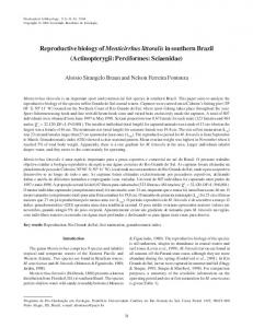
Proving WD can be seen as filtering out proof obligations containing ill-defined expressions. For instance, for ‘` pred (0) = pred (0)’ we are additionally required to prove ‘` 0 6= 0 ∧ 0 6= 0’ as its WD (this proof obligation is computed using definitions that appear in §4.4 and §4.5.1). Since this is not provable, we have filtered out (and therefore rejected) ‘` pred (0) = pred (0)’ as not being well-defined in the same way as we would have filtered out and rejected ‘` 0 = ∅’ as not being well-typed. Well-definedness though, is undecidable and therefore needs to be proved. Figure 4.1 illustrates how well-definedness can be thought of as an additional proof-based filter for mathematical texts.

Mathematical text to prove

Lexical analysis

Syntactic analysis

Static filters

Type checking

Well definedness

Validity

Proof-based filter

Figure 4.1: Well-definedness as an additional filter

When proving Validity, we may then additionally assume that the initial sequent ‘H ` G’ is well-defined. The assumption that a sequent is welldefined can be used to greatly ease its proof. It allows us to avoid proving that a formula is well-defined every time we want to use it (by expanding its definition, or applying its derived rules) in our proof. For instance we may apply the simplification rule ‘x 6= 0 ` pred (x + y) = pred (x) + y’ without proving its premise ‘x 6= 0’. This corresponds to the way a mathematician works. In §4.5.4 we show this key result formally; i.e. how conditional definitions become ‘unconditional’ for well-defined sequents. For the moment though, we may only assume that the initial sequent of Validity is well-defined. In order to take advantage of this property throughout a proof we need to use proof rules that preserve well-definedness. Preserving well-definedness in an interactive proof also has the advantage of preventing the user from introducing possibly erroneous ill-defined terms into a proof. A proof calculus preserving well-definedness is presented in §4.5. Before that, in the next section, we first introduce the well-definedness operator.


4.4

The Well-Definedness Operator

The WD operator ‘D’ formally encodes what we mean by well-definedness. D is a syntactic operator (similar in status to the substitution operator ‘[x := E]’ seen in §3.4.5) that maps formulæ to their well-definedness (WD) predicates. We interpret the predicate denoted by D(F ) as being valid iff F is well-defined. The D operator is attributed to Kleene [61] and also appears in [10, 25, 26, 36], and as the ‘δ’ operator in [19, 45]. Since D has been previously well studied, we only give in this section an overview of the properties of D from [10] that we use later in this chapter. In §4.4.1 we define D for formulæ in basicFoPCe. In §4.4.2 we derive equivalences that allow D for all formulæ in FoPCe to be computed, and state an important properties of D that we use later in §4.5.

4.4.1

Defining D

D is defined on the structure of formulæ in basicFoPCe using syntactic definitions. For expressions, D is defined as follows:

D(x) = b > ~ ~ E) ~ ∧ Cf D(f (E)) = b D( ~ E

(4.1) (4.2)

~ is D extended for sequences of formulæ (i.e. D( ~ )= ~ where D b >, D(F, F~ ) = b ~ ~ D(F )∧D(F )). An occurrence of a variable in a formula is always well-defined. The occurrence of a function application is well-defined iff all its operands ~ holds), and the well-definedness condition ‘C f ’ ~ E) are well-defined (i.e. D( ~ E from the conditional definition of f holds. The resulting definition for the running example ‘pred’ is: D(pred (E)) = b D(E) ∧ E 6= 0 Similarly, D for ⊥, ¬, = and relational predicate application is defined as follows:

D(⊥) D(¬P ) D(E1 = E2 ) ~ D(R(E))

= b > = b D(P ) = b D(E1 ) ∧ D(E2 ) ~ E) ~ = b D(

(4.3) (4.4) (4.5) (4.6)

4.4. THE WELL-DEFINEDNESS OPERATOR

41

Note that we regard relational predicate application as always being total. In case we require partial relational predicate symbols, they can be supported in the same way as partial function symbols. Since we would like predicates such as ‘x 6= 0 ∧ pred (x) = x’ (or similarly, ‘x 6= 0 ⇒ pred (x) 6= x’) to be well-defined special care is taken while defining the well-definedness of ∧ and ∀ as follows:

D(P ∧ Q) = b (D(P ) ∧ D(Q)) ∨ (D(P ) ∧ ¬P ) ∨ (D(Q) ∧ ¬Q) (4.7) D(∀x·P ) = b (∀x·D(P )) ∨ (∃x·D(P ) ∧ ¬P ) (4.8) Intuitively, the above definitions enumerate all the possible conditions where a conjunctive or universally quantified predicate could be well-defined. A formal derivation of these definitions can be found in [10]. From these definitions we can see that D is itself total and can always be eliminated from any formula.

4.4.2

Proving properties about D

All proofs done in this chapter use the standard predicate calculus FoPCe. When we say that a predicate ‘P ’ is valid or provable, we mean that we have a proof of the sequent ‘ ` P ’ using FoPCe. In this section (and in §4.5.4) we show some important logical (as opposed to syntactic) properties about D. Care must be taken when proving statements that contain both syntactic and logical operators. Since D is not a logical operator, but a syntactic one, modifying its argument using standard logical transformations is not valid. For instance, given that ‘P ⇔ Q’ holds (i.e. is valid in FoPCe), it is wrong to conclude that ‘D(P ) ⇔ D(Q)’ (consider the valid predicate ‘> ⇔ pred (0) = pred (0)’). The only modifications that can be made to the arguments of D are purely syntactic ones, such as applying syntactic rewrites (using syntactic definitions that use ‘=’). b In this section we state some properties of D. D of WD predicates An important property of D is that for any formula F,

D(D(F )) ⇔ >

(4.9)

This means that all WD predicates are themselves well-defined . This property can be proved by induction on the structure of basic formulæ. A proof

42 CHAPTER 4. PARTIAL FUNCTIONS AND WELL-DEFINEDNESS of this nature can be found in the appendix of [10]. Note that the above property is expressed in terms of logical equivalence ‘⇔’ and not syntactic definition ‘=’. b D for Derived Logical Operators The following equivalences can be used to compute the WD predicates of the derived logical operators >, ∨, ⇒, ⇔ and ∃: D(>) D(P ∨ Q) D(P ⇒ Q) D(P ⇔ Q) D(∃x·P )

⇔ ⇔ ⇔ ⇔ ⇔

> (D(P ) ∧ D(Q)) ∨ (D(P ) ∧ P ) ∨ (D(Q) ∧ Q) (D(P ) ∧ D(Q)) ∨ (D(P ) ∧ ¬P ) ∨ (D(Q) ∧ Q) D(P ) ∧ D(Q) (∀x·D(P )) ∨ (∃x·D(P ) ∧ P )

(4.10) (4.11) (4.12) (4.13) (4.14)

The statements above can be proved using FoPCe (considering the discussion in §3.3.7 and the precautions stated in the beginning of this section) after unfolding the definitions of the derived logical operators and D.

4.5

Well-Definedness and Proof

This section contains the main contribution of this chapter. The theme of §4.4 was the well-definedness of individual formulæ. In this section we show how the notion of well-definedness can be integrated into proofs (i.e. sequents and proof rules). In §4.5.1 we define D for sequents. We then formally define the notions of a well-defined sequent (§4.5.2) and a WD preserving proof rule (§4.5.3) as motivated in §4.3. In §4.5.4 we derive the proof calculus FoPCe D , the WD preserving version of FoPCe, that we use to preserve well-definedness in a proof. We summarise the results of this section in §4.5.5.

4.5.1

Defining D for Sequents

We now extend our definition V of D to sequents. Observing that the sequent ‘ H ` G ’ is valid iff ‘ ` ∀~x. H ⇒ G ’ is also valid (where ‘∀~x’ denotes the V universal quantification of all free variables occurring in H and G, and ‘ H’ denotes the conjunction of all predicates present in H), we extend our well-definedness operator to sequents as follows: D( H ` G )

= b

D( ∀~x.

^

H ⇒ G)

(4.15)

4.5. WELL-DEFINEDNESS AND PROOF

43

Note that if we blindly use the definitions (4.15), (4.8), (4.12), and (4.7) to evaluate ‘D( H ` G )’ we get a disjunctive predicate that grows exponentially with respect to the number of free variables and hypotheses in the sequent. We present ways to overcome this problem in §4.5.2.2 and §4.6.

4.5.2

Well-Defined Sequents

In §4.3 we said that the initial sequent of the Validity proof obligation could be considered well-defined since we also prove WD. More generally, we say that a sequent ‘H ` G’ is well-defined if we can additionally assume ‘D( H ` G )’ to be present in its hypotheses. We thereby encode the well-definedness of a sequent within its hypotheses. We introduce additional syntactic sugar ‘`D ’ to denote such a well-defined sequent:

H `D G 4.5.2.1

= b

D( H ` G ), H ` G

(4.16)

Re-stating WD and Validity

We may re-state our original proof obligations from §4.3 in terms of ‘`D ’ as follows: WDD : `D D( H ` G )

ValidityD :

H `D G

Justification The WDD proof obligation is equivalent to the original WD proof obligation since we know from (4.9) that ‘D(D(H ` G)) ⇔ >’. To get ValidityD , we add the extra hypothesis ‘D( H ` G )’ to Validity using the cut rule whose first antecedent can be discharged using the proof of WD. We return to the issue of proving WDD and ValidityD in §4.6. The rest of this section is concerned with proving well-defined ‘`D ’ sequents in general. 4.5.2.2

Simplifying `D

Directly unfolding (4.16) introduces the predicate ‘D( H ` G )’ that, as we have seen in §4.5.1, grows exponentially when further unfolded. We avoid unfolding ‘D( H ` G )’ by using the following derived rule instead of (4.16) to introduce or eliminate `D from a proof : b D(H), D(G), H ` G `D eqv H `D G

44 CHAPTER 4. PARTIAL FUNCTIONS AND WELL-DEFINEDNESS S b operator is D extended for finite sets of formulæ (i.e. D(F) b The D = b F ∈F {D(F )}). b Note that D(H) denotes a set of predicates. The double inference line means that this rule can be used in both directions. The rule `D eqv says that when proving the validity of a well defined sequent, we may assume that all its hypotheses and its goal are individually well-defined. Proof of `D eqv We will use the following three derived rules as lemmas in order to prove `D eqv : D(P ) ` P ∀ D(∀x·P ) ` ∀x·P D

D(P ), D(Q), P ` Q ⇒D D(P ⇒ Q) ` P ⇒ Q

H, D(P ), D(Q), P, Q ` R ∧D H, D(P ∧ Q), P ∧ Q ` R The proofs of ⇒D and ∧D in both directions are straightforward using the definitions of D and the rules of FoPCe, and are similar to the proof of ` D eqv simple shown later in this section. The proof of ∀D though is tricky, but almost identical to the proof of another derived rule ∀goal D presented in §4.5.4.1. The proof of `D eqv proceeds as follows. The logical content of the sequent (i.e. the hypotheses and the goal) is first packed into the goal of the sequent using the rules of FoPCe. This goal is then unraveled in parallel with its well-definedness predicate using the three derived rules stated above. Here is the proof: b D(H), D(G), H ` G `D eqv H `D G b D(H), D(G), H ` G V V ∧|H| D( H), D(G), H ` G D ⇒D V V D( H ⇒ G ) ` H ⇒ G x| V V ∀|~ D D( ∀~x · H ⇒ G ) ` ∀~x · H ⇒ G V (4.15) D( H ` G ) ` ∀~x · H ⇒ G FoPCe D( H ` G ), H ` G (4.16) H `D G Superscripts above the rules ∀D and ∧D indicate the number of applications x| of these rules. For instance ∀|~ indicates |~x| (which is the number of free D


45

variables in the original sequent) applications of the rule ∀D . Note that this is allowed since the number of free variables (|~x|) and hypotheses (|H|) contained in a sequent are finite. In what follows we try to give the reader intuition on why `D eqv is valid since this cannot be easily seen from the proof just presented. The fact that `D eqv holds in the downward direction (i.e. if the hypotheses and goal of a sequent are well-defined, then the sequent as a whole is well-defined) is easy to see since hypotheses are weakened. For the upward direction, we present the proof of the simpler case where the well-defined sequent has no free variables and only one hypothesis. The derived rule corresponding to this simple case appears boxed on the right, followed by its proof: D(H), D(G), H ` G `D eqv simple H `D G ¬hyp; hyp hyp D(H), D(G), H ` G D(H), ¬H, H ` G D(G), G, H ` G FoPCe (D(H) ∧ D(G)) ∨ (D(H) ∧ ¬H) ∨ (D(G) ∧ G), H ` G (4.12) D(H ⇒ G), H ` G (4.16); (4.15) H `D G From the proof above we can see that, apart from the case where the hypothesis and the goal are individually well-defined, all other possible cases in which the sequent could be well-defined (i.e. the remaining disjuncts of ‘D(H ⇒ G)’) can be discharged using the rules in FoPCe.

4.5.3

WD preserving Proof Rules

We say that a proof rule preserves well-definedness iff its consequent and antecedents only contain well-defined sequents (i.e. `D sequents). Examples of WD preserving proof rules can be found in §4.5.4. We may derive such rules by first using `D eqv to rewrite `D sequents in terms of ‘`’ and then use FoPCe and the properties of D to complete the proof. Such proofs are discussed in detail in §4.5.4.1.

4.5.4

Deriving FoPCe D

We now have enough formal machinery in place to derive the WD preserving proof calculus FoPCe D . For each proof rule ‘r’ in FoPCe we derive its WD preserving version ‘rD ’ that only contains sequents using ‘`D ’ instead of ‘`’. Here are the resulting proof rules for basicFoPCe D that are (apart from the `D turnstile) identical to their counterparts in basicFoPCe:


H, P `D P

H, ⊥ `D P

H `D Q mon D H, P `D Q

hyp D ⊥hyp D

H, ¬P `D ⊥ contr D H `D P

H, P `D ⊥ ¬goal D H `D ¬P

H `D P H `D Q ∧goal D H `D P ∧ Q

H `D P ¬hyp D H, ¬P `D Q

H, P, Q `D R ∧hyp D H, P ∧ Q `D R

H `D P ∀goal D (x nfin H) H `D ∀x·P

H `D E = E

= goal D

H `D [x := E]P = hyp D H, E = F `D [x := F ]P

The remaining rules, cut and ∀hyp, need to be reformulated by adding new antecedents (that appear boxed below) to make them WD preserving: H `D D(P)

H `D P

H, P `D Q

H `D Q H `D D(E)

H, [x := E]P `D Q

H, ∀x·P `D Q

cut D

∀hyp D

These new antecedents are WD sub-goals that need to be discharged when these rules are used in a proof. The original rules (cut and ∀hyp) are not WD preserving since they introduce new predicates and expressions that may be ill-defined into a proof. Note that the converse is not true. A valid proof rule in FoPCe that does not introduce any new formulæ into a proof can be non WD preserving. The following derived proof rule illustrates this: H`P H, P ` Q H`P ∧Q Although this rule is valid (it can be proved using ∧goal and cut) and does not introduce any new formulæ, it does not preserve well-definedness. The first antecedent would be ill-defined in the case where P (say ‘pred (x) = 0’) is only well-defined in conjunction with Q (say ‘x 6= 0’). The proofs of the rules of basicFoPCe D are discussed later in §4.5.4.1.


47

Derived Logical Operators Once we have derived the rules of basicFoPCe D stated above, we may use them directly (i.e. without the detour through ` sequents) to derive the corresponding WD preserving proof rules for the derived logical operators >, ∨, ⇒, ⇔ and ∃ that appear below: H `D > H `D P ∨goal 1D H `D P ∨ Q

>goal D

H `D Q ∨goal 2D H `D P ∨ Q

H, P `D Q ⇒goal D H `D P ⇒ Q

H, P `D R H, Q `D R ∨hyp D H, P ∨ Q `D R

H `D P H, Q `D R ⇒hyp D H, P ⇒ Q `D R

H `D P ⇒ Q H `D Q ⇒ P ⇔goal D H `D P ⇔ Q

H, P ⇒ Q, Q ⇒ P `D R ⇔hyp D H, P ⇔ Q `D R

H `D D(E)

H, P `D Q ˆ ∪ {Q}) ∃hyp D (x nfinH H, ∃x·P `D Q

H `D [x := E]P

H `D ∃x·P

∃goal D

The only rule here that needs modification is the existential dual of ∀hyp (i.e. ∃goal ). The resulting proof rules constitute our complete WD preserving proof calculus FoPCe D . Conditional Definitions The payoff achieved by using FoPCe D instead of FoPCe in proofs is that conditional definitions in FoPCe become ‘unconditional’ in FoPCe D . The ‘`D ’ version of the fdef rule from §4.2 is: `D y = f (~x) ⇔ D~xf ,y

fdef D

The above rule differs from fdef in that it does not explicitly require the WD condition ‘C~xf ’ in order to be applied, simplifying proofs. The above rule can

be derived from fdef since D 4.5.4.1

y = f (~x) ⇔ D~xf ,y ⇒ C~xf .

Proofs of basicFoPCe D

The proofs of each rule in basicFoPCe D that appear in §4.5.4 follow essentially from `D eqv , the properties of D, and the rules in FoPCe. Since some of the proofs are not straightforward we outline some of their major steps in this section as an aid the reader who wants to reproduce them. This section may otherwise be skipped.

48 CHAPTER 4. PARTIAL FUNCTIONS AND WELL-DEFINEDNESS The proofs of hyp D , ⊥hyp D and = goal D are trivial since these rules contain no antecedents. In general, any valid rule having no antecedents is trivially WD preserving. The proofs for mon D , contr D , ¬goal D , ¬hyp D , and ∧hyp D are straightforward and similar in style to the proof of cut D shown below: H `D D(P )

H `D D(P )

H `D P

H `D P H `D Q

H, P `D Q

cut D

H, P `D Q

cut (P ) ; `D eqv b b D(H), D(Q), H ` D(P ) D(H), D(Q), H, D(P ) ` Q cut (D(P )) b D(H), D(Q), H ` Q `D eqv H `D Q The proofs of ∀hyp D and = goal D require the following additional properties about how D interacts with the substitution operator: (4.9); `D eqv

D([x := E]F ) ⇒ [x := E]D(F ) ([x := E]D(F )) ∧ D(E) ⇒ D([x := E]F )

(4.17) (4.18)

Both these properties can be proved by induction on the structure of basic formulæ. The proofs of ∧goal D and ∀goal D are tricky and require rewriting definitions (4.7) and (4.8) as follows:

D(P ∧ Q) ⇔ (D(P ) ∧ (P ⇒ D(Q))) ∨ (D(Q) ∧ (Q ⇒ D(P )))(4.19) D(∀x·P ) ⇔ ∃x· (D(P ) ∧ (P ⇒ ∀x·D(P ))) (4.20) Using these equivalences instead of (4.7) and (4.8) allows for more natural case splits in these proofs. The proof of ∧goal D is similar to the proof of ∀goal D shown below: H `D P ∀goal D (x nfin H) H `D ∀x·P

4.6. PROVING WDD AND VALIDITYD

49 H `D P

∀hyp; `D eqv b D(H), ∀x·D(P ), H ` P ∀goal (x nfin H) b H `D P D(H), ∀x·D(P ), H ` ∀x·P mon (D(P )) `D eqv b b D(H), D(P ), H ` P D(H), D(P ), ∀x·D(P ), H ` ∀x·P ⇒hyp b D(H), D(P ), P ⇒ ∀x·D(P ), H ` ∀x·P ∃hyp; ∧hyp b D(H), ∃x·(D(P ) ∧ (P ⇒ ∀x·D(P ))), H ` ∀x·P `D eqv ; (4.20) H `D ∀x·P We now summarise the results of this section.

4.5.5

Summary

In this section we have shown how the notion of well-definedness can be integrated into proofs by extending the definition of D to sequents (§4.5.1), and characterising well-defined ‘`D ’ sequents (§4.5.2). We have derived the proof rule `D eqv (§4.5.2.2) that allows us to freely move between ordinary ‘`’ sequents and well-defined ‘`D ’ sequents in proofs. We have formally derived the proof calculus FoPCe D (§4.5) whose rules preserve well-definedness. The rules of FoPCe D are identical to those in FoPCe except for three cases (cut, ∀hyp and ∃goal ) where additional WD sub-goals need to be proved. We now return to the practical issue of proving the WD and Validity proof obligations introduced in §4.3.

4.6

Proving WDD and ValidityD

In §4.5.2.1 we re-stated our original proof obligations from §4.3 in terms of ‘`D ’ as follows: WDD : `D D( H ` G )

ValidityD :

H `D G

Proving WDD In our practical setting we factor out proving WDD for each proof obligation individually by proving instead that the (source) models used to generate these proof obligations are well-defined. Details on welldefinedness of models can be found in [25]. We are guaranteed that all proof obligations generated from a well-defined model are themselves well-defined and therefore do not need to generate or prove the well-definedness of each proof obligation individually. This considerably reduces the number of proofs that need to be done.

50 CHAPTER 4. PARTIAL FUNCTIONS AND WELL-DEFINEDNESS Proving ValidityD From the ‘`D ’ turnstile we immediately see that the initial sequent of ValidityD is well-defined. We have two choices for how to proceed with this proof. We may either use FoPCe D to preserve well-definedness, or the standard FoPCe. We prefer using the WD preserving calculus FoPCe D (with additional WD sub-goals) instead of FoPCe for interactive proofs for three reasons. Firstly, as seen in §4.3, the assumption that a sequent is well-defined can be used to greatly ease its proof. Secondly, the extra WD sub-goals require only minimal additional effort to prove in practice, and are in most cases automatically discharged. Thirdly, proving WD sub-goals allows us to filter out erroneous ill-defined formulæ entered by the user. Alternatively, we may use the rule ` D eqv (§4.5.2.2) to make the welldefinedness assumptions of a ‘`D ’ sequent explicit and use the standard proof rules in FoPCe to complete a proof. This may not be a prudent way to perform interactive proof, but it allows us to use existing automated theorem provers for FoPCe (that do not have any notion of well-definedness) to automatically discharge pending sub-goals.

4.7

Related Work

A lot of work has been done in the area of reasoning in the presence of partial functions. A good review of this work can be found in [51] and [10]. In this section we first describe some approaches that are most relevant to the work presented in this chapter and then compare our work to these approaches in §4.7.1. The current approaches to reason about the undefined can be classified into two broad categories: those that explicitly reason about undefined values using a three-valued logic [61], and those that avoid reasoning about the undefined using underspecification. We start with the former. A well known approach is the Logic of Partial Functions (LPF) [57, 19] used by the VDM [56] community. Its semantics is based on three-valued logic [61]. The resulting proof calculus for LPF can then be used to simultaneously prove the validity and well-definedness of a logical statement. A drawback of using LPF (or any other special-purpose proof calculus) is that it differs from the standard predicate calculus since it disallows use of the law of excluded middle (to avoid proving ‘3/0 = x ∨ 3/0 6= x’) and additionally requires a second ‘weak’ notion of equality (to avoid proving ‘3/0 = 3/0’). Additional effort is therefore needed to learn or automate LPF, as for any special-purpose proof calculus, as mentioned in §4.1.

4.7. RELATED WORK

51

In PVS [74], partial functions are modelled as total functions whose domain is a predicate subtype. For instance, the partial function ‘/’ is defined as a total function whose second argument belongs to the subtype of nonzero reals. Type-checking then avoids ill-definedness but requires proof. The user needs to prove type correctness conditions (TCCs) before starting or introducing new formulæ into a proof. A shortcoming of this approach is that type-checking requires complicated typing rules [75] and special tool support. This approach additionally blurs the distinction between type-checking (which is usually accepted to be automatically decidable) and proof. In [25], Behm et al. use a three-valued semantics to develop a proof calculus for B [3]. Its main difference from LPF is that the undefined value, although part of the logical semantics, does not enter into proofs, as explained below. In this approach, all formulæ that appear in a proof need to be proved to be well-defined. Proving well-definedness is similar to proving TCCs in PVS. It has the role of filtering out expressions that may be illdefined. Once this is done, the proof may continue in a pseudo-two-valued logic since the undefined value is proved never to occur. The drawback of this approach is similar to that of LPF. Although the proof calculus presented for this pseudo-two-valued logic “is close to the standard sequent calculus”[25], this too is a special-purpose logic. No concrete connection with the standard predicate calculus is evident since this approach, from the start, assumes a three-valued semantics. In [10], Abrial and Mussat formalise the notion of well-definedness without any detour through a three-valued semantics, remaining entirely within the “syntactic manipulation of proofs”[10] in standard predicate calculus. The resulting well-definedness filter is identical to that in [25]. They formally show how proving statements that passed this filter could be made simpler (i.e. with fewer checks) on the basis of their well-definedness. What is missing in [10] however is a proof calculus (like the one in [25]) that preserves well-definedness, which could additionally be used for interactive proof. In [26], Berezin et al. also use the approach of filtering out ill-defined statements before attempting to prove them in the automated theorem prover CVC lite. The filter used is identical to the one used in [25] and [10]. Although they too start from a three-valued logic, they show (using semantic arguments) how the proof of a statement that has passed this filter may proceed in standard two-valued logic. Apart from introducing three-valued logic only to reduce it later to two-valued logic, this approach is concerned with purely automated theorem proving and therefore provides no proof calculus that preserves well-definedness to use in interactive proofs. It is advantageous to preserve well-definedness in interactive proofs (reasons for this are given in §4.3).

52 CHAPTER 4. PARTIAL FUNCTIONS AND WELL-DEFINEDNESS The idea of avoiding reasoning about undefined values using underspecification [51] is used in many approaches that stick to using two-valued logic in the presence of partial functions. This is the approach used in Isabelle/HOL [73], HOL [49], JML [31] and Spec# [18]. In this setting, an expression such as ‘3/0’ is still a valid expression, but its value is unspecified. Although underspecification allows proofs involving partial functions to be done in two-valued logic, it has two shortcomings. First, (as described in §4.2) it also allows statements that contain ill-defined terms such as ‘3/0 = 3/0’ to be proved valid. In the context of generating or verifying program code, expressions such as ‘3/0’ originating from a proved development can lead to a run-time error as described in [31]. Second, doing proofs in this setting may require repeatedly proving that a possibly undefined expression (e.g. ‘3/x’) is actually well defined (i.e. that ‘x 6= 0’) in multiple proof steps.

4.7.1

Comparison

In this section we compare the approach presented in this chapter (§4.4, §4.5) with the related work just presented. The work presented here extends the approach of [10] by showing how the notion of well-definedness can be integrated into a proof calculus that is suitable for interactive proof. The role of proving TCCs in PVS is identical to that of proving welldefinedness in our approach (i.e. proving the WD proof obligation and the additional WD sub-goals in cut D , ∀hyp D , and ∃goal D ). With regards to its logical foundations, we find the possibility of directly defining truly partial functions in our setting more convenient and intuitive as opposed to expressing them as total functions over a restricted subtype. The logical machinery we use is much simpler too since we do not need to introduce predicate subtypes and dependent types for this purpose. Since we use standard (decidable) type-checking we have a clear conceptual separation between type-checking and proof. Although our approach does not eliminate the undecidability of checking well-definedness, it saves type checking from being undecidable. With respect to B [25] and LPF [19], the approach used here does not start from a three-valued semantics but instead reduces all reasoning about well-definedness to standard predicate calculus. We develop the notion of well-definedness purely on the basis of the syntactic operator ‘D’ and proofs in standard predicate calculus. In §4.5 we derive a proof calculus preserving well-definedness that is identical to the one presented in [25]. Alternatively, we could have chosen to derive the proof calculus used in LPF in a similar fashion. If our definition of well-defined sequents is modified from the one appearing in §4.5.2 to

4.7. RELATED WORK

H `LPF G

53

= b

b D(H), H ` G ∧ D(G)

(4.21)

the rules that follow for a proof calculus that preserves ‘`LPF ’ correspond to those in LPF [19]. The only difference between ‘`LPF ’ and ‘`D ’ is that the latter also assumes the well-definedness of the goal, whereas this has to be additionally proved for ‘`LPF ’. We therefore have a clear basis to compare these two approaches. In LPF, well-definedness and validity of the goal are proved simultaneously, whereas in [25] (and also as presented in §4.3), these two proofs are performed separately, where proving WD acts as a filter. Since what is proved is essentially the same, the choice of which approach to use is a methodological preference. We use the latter approach although it requires proving two proof obligations because of four reasons. First, the majority of the WD sub-goals that we encounter in practice (from models and interactive proof steps) are discharged automatically. Second, failure to discharge a proof obligation due to ill-definedness can be detected earlier and more precisely, before effort is spent on proving validity. Third, the structure of ‘`D ’ sequents allows us to more directly use the results in [10] and [26] to automate proofs. Fourth, we find FoPCe D more intuitive to use in interactive proofs since its rules are ‘closer’ to the standard sequent calculus (only three rules need to be modified with an extra WD sub-goal). An additional contribution over [25] (and [19]) is that we may, at any time, choose to reduce all our reasoning to standard predicate calculus (using the `D eqv rule derived in §4.5.2.2). This is a choice that could not be taken in [25]. We now compare our work to related approaches that use underspecification [51]. As described in §4.2, underspecification is the starting point from which we develop our approach. The work presented in this chapter can be used to overcome two of the shortcomings the underspecification approach mentioned earlier. First, (as discussed in §4.3) proving the well-definedness of proof obligations (or of the source model) gives us an additional guarantee that partial (underspecified) functions are not evaluated outside their domain in specifications or program code. This has been recently done along similar lines for Spec# [18] in [83]. Second, (as discussed in §4.3 and §4.5.3) preserving well-definedness in proofs allows us to avoid having to prove well-definedness repeatedly, every time we are confronted with a possibly ill-defined expression during proof.


4.8

Conclusion

In this chapter we have shown how standard predicate calculus can be used to reason in a setting with potentially ill-defined expressions by extending it with new syntax and derived rules for this purpose. The results presented in §4.5 provide a deeper understanding of reasoning in the context of well-definedness, and its connection with the standard predicate calculus. This work has also resulted in providing better tool support for proving within the RODIN development environment [1] for Event-B.

Chapter 5 Prover Architecture and Extensibility In this chapter we present the basic architecture of the proof tool and the ways in which its proving capabilities can be extended. For clarity we restrict this basic architecture to the propositional subset of our mathematical language. We show how proofs can be constructed in the proof tool, and how these constructed proofs correspond to our mathematical notion of proof discussed in chapter 3. The implementation of the proof tool is sketched using an object-oriented pseudo-code notation. This chapter provides a concrete basis for the discussions in chapters 6, 7, and 8.

5.1

Introduction

The proof tool is a computer program that implements the mathematical logic described in chapter 3, the latter being its formal specification. The main aim of the proof tool is to allow us to discharge proof obligations, which are sequents as described in §3.3.2. A proof obligation can be discharged by constructing a proof for it as described in §3.2.4. A proof constructed in the tool is a reflection of its mathematical sequent-style proof. Before starting, it is appropriate to mention that the proof tool proposed in this chapter, and the rest of this thesis is not a meta-prover able to be parametrized by a variety of distinct logics such as Isabelle [78]. It is neither a Logical Framework such as ELF [53] or Twelf [86] designed to be used for studying the properties of a given logical system. The prover described here is meant to be a practical tool aimed at discharging proof obligations using a specific mathematical logic, in our case the one described in chapter 3. The key points of the proof tool that will be covered in this chapter are: 55

56

CHAPTER 5. PROVER ARCHITECTURE AND EXTENSIBILITY The main data-structures and algorithms used. The extension mechanisms used. How proofs are constructed. The correspondence between proofs constructed using the tool and proofs in the mathematical logic described in chapter 3.

Special importance is given to extensibility of the proof tool. In particular, a central point in its design was to allow external automated theorem provers to be easily integrated within the proof tool. As described in [38], [68] and [67] reusing the reasoning capabilities of off-the-shelf automated theorem provers has been observed to be very advantageous for program varification tasks. The next section gives an informal overview of the proof tool architecture, with emphasis on how the proof tool can be extended.

5.2

Prover Extensibility

A central requirement of our proof tool is that its reasoning capabilities should be extensible. By this we mean that it should be possible to add commonly used derived proof rules or automated decision procedures into the repertoire of the proof tool and use them when constructing proofs. In order to allow for this type of extensibility, we choose a modular architecture where we separate the extensible parts of the proof tool, responsible for generating individual proof rules, from the static part responsible for putting proof rules together to construct and manage proofs. The ‘trusted code-base’ of the proof tool comprises of: a. A collection of Reasoners that are responsible for generating valid proof rules. b. The Proof Manager which is responsible for putting these generated rules together to construct a valid proof. The basic reasoning capabilities of the proof tool can be extended by adding new reasoners to it. A reasoner may for instance implement a decision procedure for automated proof, or a derived rule schema for interactive proof. The main point to note here is that (in contrast to most currently used proof tools as discussed in §5.11) the internal workings of an individual reasoner are not visible to the rest of the proof tool. It is only required that a reasoner

5.3. THE BASIC PROVER ARCHITECTURE

57

satisfies a minimal set of requirements (stated in §5.8.1) in order to guarantee soundness of the proof tool. It is therefore possible to integrate external theorem provers into the proof tool with very little effort. Reasoners are described in detail in §5.8. The proof tool also provides tactics that encapsulate frequently used proof construction and manipulation steps. Tactics provide a convenient way to structure high-level strategic or heuristic knowledge about proof search and manipulation. They provide control structures to call reasoners or other tactics to modify entire proofs. Tactics are described in detail in §5.10. The second way to extend the proof tool is to add new tactics to it. In contrast to reasoner extensions, tactic extensions are easier to write and do not compromise the soundness of the proof tool.

5.3

The Basic Prover Architecture

In the rest of this chapter we present the architecture of the proof tool in greater detail and sketch its implementation. In order to bring out the main points clearly, we do not present the actual implementation of the proof tool, but instead present its basic architecture which differs from its actual implementation on two points as described in the paragraphs that follow. First, we restrict ourselves to the propositional subset of our mathematical language (which is summarised in §3.3.8) in order to bring out the key ideas behind the proof tool in a simpler setting. The implemented proof tool supports the complete mathematical language, including well-definedness as described in chapter 4 and can be found online at [2]. The major addition required in order to support the complete mathematical language is the treatment of free and bound variables. This is both well understood and straightforward to incorporate by adding additional non-freeness checks and dependencies to the pseudo-code shown here, but has been omitted in our presentation to increase its clarity. Second, we use an object-oriented pseudo-code notation (that we are about to introduce in §5.4) for presentation. The main aim of using this notation is to communicate the design and implementation of the proof tool in a way that is clear and simple, in the spirit of how many textbooks on algorithm design present their implementations. We avoid showing the actual Java [50] implementation to avoid cluttering our presentation with language specific artifacts that have no relevance here. Although it would have been possible to use an established formal modeling notation (such as the Event-B notation supported by the RODIN tool)

58

CHAPTER 5. PROVER ARCHITECTURE AND EXTENSIBILITY

this has not been done since: We would like to base our discussions on the actual implementation of the proof tool, and not on a model of its actual implementation. A formal specification of the proof tool (i.e. what it means for a proof to be valid) is already covered in chapter 3. Using such a formal model would require us to additionally argue about how faithful the actual implementation is to the model. Some amount of clarity would be sacrificed in translating the inherently object oriented concepts used here to those of the modeling notation.

That having been said, we incorporate some ideas (such as invariants, pre-conditions and post-conditions) from formal modeling notations such as JML [63] and Event-B in order to express properties of the pseudo-code we present. The main disadvantage of using pseudo-code in this respect is that we cannot mechanically prove that these properties hold. The complete Java implementation of the proof tool that supports the entire mathematical language, including well-definedness as described in chapter 4, can be found online at [2].

5.4

Programing Notation

This section describes the programing notation used to present data-structures and algorithms in the rest of this thesis. The proof tool is implemented in the object-oriented programing language Java [50]. In order to avoid going into implementation details, while still remaining faithful to the implementation we use an object-oriented pseudo-code notation for presentation purposes. What follows is a short description of the main points of this notation. A class is the basis of modularity and structure in an object-oriented setting. A class defines a unit consisting of a data specification and its behaviour. Its data specification is defined by its attributes, and its behaviour is defined by its methods. Here is an example of a class definition for Point with two integer attributes: 1 2 3 4

class Point{ int x; int y; }

5.4. PROGRAMING NOTATION

59

An object is an instance of a class. We use the following notation to declare and construct objects of a particular class: 1

Point origin := PointL x := 0, y:=0 M;

The object origin is said to have the type Point. We define the method divide for the class Point as follows: 1 2 3 4 5 6 7 8 9 10

boolean Point::divide(int i){ if (i = 0){ return false; } else{ this.x := this.x ÷ i; this.y := this.y ÷ i; return true; } }

Line 1 contains the signature of the method. It says that this method returns a boolean and accepts the integer parameter ‘i’ as input. The ‘Point::’ before the method name indicates that this method belongs to the Point class. The above method can be invoked on the object origin of type Point with the input parameter ‘0’ using the method call notation ‘origin.divide(0)’. The body of the method (lines 2 to 9) is an imperative program. It first checks if i equals 0 (line 2) and returns false if this is the case (line 3). Otherwise it modifies the attributes of the invoking object by dividing them by i (lines 6 and 7) and returns true (line 8). The keyword ‘this’ in the method body is used to access and modify the attributes of the invoking object. We declare an attribute of a class as being immutable if this attribute is not allowed to be modified after its construction. Declaring a class to be immutable makes all its attributes immutable. The types int and boolean are used for integer and boolean values respectively. We assume that we have the type constructors ‘[]’ for lists, and ‘{}’ for sets of objects of a particular type. We use the syntax ‘Point[]’ and ‘Point{}’ to denote the type of lists and sets of Point objects respectively. Lists and sets of objects are declared and constructed using the following notation: 1 2

Point[] pointList := [point1, point2, point3]; Point{} pointSet := {point1, point2, point3};

We use the square bracket notation ‘pointList[i]’ to access the ith element of pointList. List indices start at 0. We use ‘pointList.length’ to access the length of pointList. We also use the notation ‘pointList[i]:=point’

60


to modify the ith element of pointList, or to append an element to pointList in case its current length is i. We use the expression ‘[]’ to denote the empty list, and the operator ‘a’ to denote list concatenation. We use ‘∅’ to denote the empty set, and use the standard mathematical notation (∈, ∈, / ⊆, 6⊆, ∪) for operations on sets. We use the equality symbol ‘=’ in the mathematical sense (i.e. deep equality, and not just referential equality) to compare two objects of the same type. As common programing practice, we sometimes use the null value to model the ends of data-structures and the return values of failed method invocations. The super-scripted type annotation ‘? ’ after a type indicates that an object of that type may be equal to null. For instance the declaration ‘Point? point’ indicates that point may be equal to null and that this needs to be checked before trying to access its attributes. An interface is an abstract class containing only method signatures. Here is an example of an interface declaration: 1 2 3

interface Dividable{ boolean divide(int i); }

We say that the class Point implements the interface Dividable since it provides the divide method with the same signature as in the interface. Interfaces are used to support extensibility of the proof tool. We now use this pseudo-code notation to describe the main data structures and algorithms used in the proof tool.

5.5

Predicates

We assume we have a class Predicate that implements the abstract syntax tree for predicates and provides methods to query and construct such predicates. The objects of type Predicate are immutable. 1 2 3

immutable class Predicate{ ... }

5.6

Sequents

A sequent is implemented as a class containing two attributes: 1

immutable class Sequent{

5.7. PROOF RULES Predicate goal; Predicate{} hyps;

2 3 4

61

}

The goal attribute refers to the single goal predicate, and hyps, to the set of hypotheses predicates. The values of both these attributes cannot be null. Additionally, the objects of type Sequent are immutable.

5.7

Proof Rules

Proof rules are implemented as objects of the following Rule class: 1 2 3 4

immutable class Rule{ Predicate usedGoal; Predicate{} usedHyps; RuleAntecedent[] ruleAntecedents;

5

Reasoner generatedBy; ReasonerInput generatedUsing;

6 7 8

}

9 10 11 12 13

immutable class RuleAntecedent{ Predicate newGoal; Predicate{} addedHyps; }

An object of type Rule is composed of a used goal predicate (usedGoal), a set of used hypotheses predicates (usedHyps), and a list of rule antecedents (ruleAntecedents of type RuleAntecedent[]). Each rule antecedent composed of a new goal predicate (newGoal), and a set of added hypotheses predicates (addedHyps). Both classes are immutable and contain only non-null attributes. The attributes generatedBy and generatedUsing in Rule are used to record the Reasoner and ReasonerInput used to generate the rule and will be described later in §5.8. Note that the representation we have chosen here for rule objects is not the same as the definition of a proof rule in the mathematical theory from §3.2.2 which states that a proof rule is composed of a consequent sequent and a list of antecedent sequents. The representation we have chosen here contains more structure and actually represents a set of ‘mathematical’ proof rules (or a proof rule schema, as we will see shortly). Using this representation not only reduces the space required to store rule objects, but also has many advantages for proof reuse as we will see in the chapter 6.

62


With respect to the mathematical theory, an object of type Rule with n rule antecedents implements the proof rule schema shown in figure 5.1 with n antecedents. H, Hu , HA0 ` GA0

Where :

Hu = usedHyps Gu = usedGoal

. . . H, Hu , HAn−1 ` GAn−1 H, Hu ` Gu HAi = ruleAntededents[i].addedHyps GAi = ruleAntededents[i].newGoal

Figure 5.1: The rule schema implemented by a rule object In this rule schema, Hu is the set of used hypotheses and Gu the used goal of the rule object. In each of its antecedents, HAi is the set of added hypotheses and GAi the new goal of the ith rule antecedent. Note that the only meta-variable in this rule schema that can be instantiated is H. Instantiating H with a set of predicates results in a concrete proof rule as defined in §3.2.2. In the tool, this instantiation is done implicitly by the Rule::apply() method below that applies a rule object to a potential consequent sequent and returns a list of antecedent sequents if successful: 1 2 3 4 5 6 7 8 9 10 11 12

Sequent[]? Rule::apply(Sequent consequent){ if (consequent.goal 6= this.usedGoal) return null; if (consequent.hyps 6⊆ this.usedHyps) return null; Sequent[] antecedents := []; for (int i := 0, i < this.ruleAntecedents.length, i++){ antecedents[i] := SequentL goal := this.ruleAntecedents[i].goal, hyps := sequent.hyps ∪ this.ruleAntecedents[i].addedHyps M; } return antecedents; }

The above method returns null if the rule is inapplicable to the given sequent. A rule is inapplicable to the given sequent if its goal is not identical to the used goal of the rule object (line 2), or the used hypotheses of the rule object are not contained in its hypotheses (line 3). In case the given sequent passes both these checks, it is an applicable consequent of the rule, and its antecedent sequents are calculated and returned (lines 4 - 11). The goal of each antecedent sequent is the new goal of the corresponding rule

5.8. REASONERS

63

antecedent (line 7). The set of hypotheses of each antecedent sequent is the union of hypotheses of the given consequent and the added hypotheses of the corresponding rule antecedent (line 8). The only proof rules (in the mathematical sense) that cannot be implemented using such rule objects are those that remove hypotheses from the consequent sequent (i.e. those proof rules that have a hypothesis in the conclusion that is not present an antecedent). Proof rules arising from the mon rule schema from §3.4.4 are examples of this. We may overlook this issue since the presence of extra hypotheses does not hinder us during proof. We have instead built the assumption that our logic is monotonic into the proof tool in the way Rule::apply() is implemented, and also in the way proofs are reused in chapter 6.

5.8

Reasoners

A reasoner is a computer program that generates Rule objects. As seen earlier in §5.2, the set of reasoners present in the proof tool is not fixed. Adding new reasoners is a way of extending the proving capabilities of the proof tool. The implementation of a reasoner is hidden from the rest of the proof tool, which allows external theorem provers to be easily integrated into our framework. Programatically, reasoners are classes that implement the following Reasoner interface: 1 2 3

interface Reasoner{ Rule? apply(Sequent sequent, ReasonerInput? input); }

4 5 6

interface ReasonerInput{ }

Each reasoner provides an apply() method that returns a Rule object in case of success, or null in case of failure. The input parameters to this method are a sequent to prove, and an optional, reasoner-specific input. Reasoners that require specialised input need to implement the empty ReasonerInput interface. Both these input parameters are mere suggestions that the reasoner may use to generate a rule. The generated rule, on the other hand, is trusted by the proof tool and therefore must conform to certain requirements that are treated in the next sub-section.

64


5.8.1

Reasoner Requirements

All rule objects generated by a reasoner need to be: a.Logically Valid By generating a rule object, a reasoner guarantees that the proof rule schema corresponding to this rule object (shown in figure 5.1) is valid (i.e. can be derived) in the mathematical logic. For the moment we assume that all reasoners present in our proof tool generate logically valid rules. In chapter 8 we will see how a rule can be checked for logical validity independent of the reasoner that generated it. b.Replayable It is also required that reasoners work deterministically, i.e. given similar inputs (a sequent with the used hypotheses and used goal, and the identical reasoner input), they generate identical rule objects. The following pseudo-code checks generated rules for this property: 1 2 3 4 5 6 7 8 9 10 11

boolean Rule::isReplayable(){ Rule? regeneratedRule := this.generatedBy.apply( SequentL goal := this.usedGoal, hyps := this.usedHyps M, this.generatedUsing ); if (regeneratedRule 6= null ∧ this = regeneratedRule) { return true; } else { return false; }; }

The above method must return true for all proof rules that satisfy the ‘replayable’ property. This method can be seen as a class invariant for rule objects, or a post-condition for the Rule::apply() method in case it generates a rule object.

5.8.2

Examples of Reasoners

We now present some examples of reasoners and show how they can be implemented within this framework. Goal in Hypotheses The following reasoner implements the hyp proof rule schema from §3.3.5 that appears just below:

5.8. REASONERS

65

H, P ` P 1

hyp

class Hyp implements Reasoner{

2

Rule? apply(Sequent sequent, ReasonerInput? input){ if (sequent.goal ∈ sequent.hyps) { return RuleL usedGoal := sequent.goal, usedHyps := {sequent.goal}, antecedents := [], generatedBy := this, generatedUsing := input M; } else { return null; } }

3 4 5 6 7 8 9 10 11 12 13 14 15 16

}

The above reasoner uses the sequent parameter as its only input. It checks the input sequent to see if its goal is present in its hypotheses (line 4). In case this is true, an appropriate rule object with no rule antecedents is returned (lines 5-11). Otherwise the reasoner fails and returns null (line 13). The proof rule schema corresponding to each rule object generated by the above reasoner is of the form: H, G ` G

Hyp()

where G is a concrete predicate (i.e. it instantiates the meta-variable P in the hyp rule schema) that is identical to the goal of the input sequent provided to the Hyp::apply() method. We use such rule schemas to represent generated rule objects more concisely on paper. We follow the convention of labeling such rule schemas using the name of the reasoner that generated it, followed by its additional input in sub-scripted brackets. The label Hyp() in the above rule schema indicates that it was generated by the Hyp reasoner using an input sequent of the form ‘H, G ` G’, without any additional input. Split Conjunctive Goal We may similarly have the following reasoner that implements the ∧goal proof rule schema from §3.3.5:

66


H`P H`Q ∧goal H`P ∧Q 1

class ConjGoal implements Reasoner{

2

Rule? apply(Sequent sequent, ReasonerInput? input){ if (sequent.goal.isConj()) { return RuleL usedGoal := sequent.goal, usedHyps := ∅, antecedents := [ AntecedentL newGoal:= sequent.goal.conjLeft(), addedHyps:= ∅ M, AntecedentL newGoal:= sequent.goal.conjRight(), addedHyps:= ∅ M ] M; } else { return null; } }

3 4 5 6 7 8 9 10 11 12 13 14 15 16 17

}

We assume we are given the method Predicate::isConj() to check if a predicate is a conjunction, and the methods Predicate::conjLeft() and Predicate::conjRight() that return the left and right conjuncts of a conjunctive predicate respectively. The proof rule schema corresponding to each rule object generated by the above reasoner is of the form: H ` G1 H ` G2 ConjGoal () H ` G1 ∧ G2 The Cut Rule A reasoner for the cut rule schema can similarly be implemented as follows: H`P

1

H, P ` Q cut H`Q

class Cut implements Reasoner{

2 3 4 5

Rule? apply(Sequent sequent, ReasonerInput? input){ if (input = null ∨ ¬(input instanceof SinglePredInput)) return null; Predicate lemma = ((SinglePredInput)input).pred;

5.8. REASONERS 6 7 8 9 10 11 12 13

}

14 15

67

return RuleL usedGoal := sequent.goal, usedHyps := ∅, antecedents := [ AntecedentL newGoal := lemma, addedHyps := ∅ M, AntecedentL newGoal := sequent.goal, addedHyps := {lemma} M ] M;

}

16 17 18 19

class SinglePredInput implements ReasonerInput{ Predicate pred; }

The main difference between this reasoner and the ones we have seen before is that it expects specialised input of the type SinglePredInput that contains the predicate to perform the cut on. This additional input is needed since it cannot be inferred from the input sequent alone. The given input is first checked to be of the correct type in line 4. The proof rule schema corresponding to each rule object generated by the above reasoner is of the form: H ` L H, L ` G Cut(L) H`G The sub-scripted predicate ‘L’ in parenthesis after the reasoner name indicates that this predicate was an additional input that was used by the reasoner to generate this rule. The next sub-section demonstrates how external theorem provers can be integrated as reasoners into the proof tool.

5.8.3

Integrating External Theorem Provers

The examples of reasoners we have seen in §5.8.2 implemented simple rule schemas in the native implementation language of the prover (in our case, the pseudo-code notation). As mentioned several times earlier, since the only requirements placed on reasoners are those stated in §5.8.1, it is also possible to integrate external off-the-shelf theorem provers as reasoners of the proof tool. The following pseudo-code shows how this can be done: 1

class ExtProver implements Reasoner{

2 3

Rule? apply(Sequent sequent, ReasonerInput? input){

68

CHAPTER 5. PROVER ARCHITECTURE AND EXTENSIBILITY boolean success := proveExternally(sequent); if (success) { return RuleL usedGoal := sequent.goal, usedHyps := sequent.hyps, antecedents := [], generatedBy := this, generatedUsing := input M; } else { return null; }

4 5 6 7 8 9 10 11 12 13 14 15

}

16 17

}

The ‘proveExternally(sequent)’ method call in line 4 calls a designated external theorem prover to discharge the given sequent, after translating it into a form suitable for the external prover, and returns true iff the external prover was successful in discharging the given sequent. In the case of success, an appropriate rule object with no rule antecedents is returned (lines 6-12). Otherwise the reasoner fails and returns null (line 14). Although the above reasoner expects no input, in practice reasoners that call external theorem provers are typically given a time-out and other prover specific inputs. In case an external prover is smart enough to return the set of hypotheses it used to perform a proof, this information can be propagated to the resulting rule object (by modifying line 5) and can be used by the proof tool to calculate proof dependencies more accurately for better proof reuse (this will be discussed later in chapter 6). Using this approach we1 were able to successfully integrate previously developed external theorem provers from the Atelier-B [33] tool into the RODIN platform. The bulk of reasoning done using RODIN is done using these automated provers. We have also successfully integrated other automated theorem provers based on the TPTP [88] syntax using this approach. In the next section we show how proof trees, the counterparts of mathematical proofs, are implemented in the proof tool.

5.9

Proof Trees

A proof tree is implemented as the following recursive data-structure: 1

This was joint work with Laurent Voisin and Fran¸cois Terrier

5.9. PROOF TREES

1 2 3 4 5

69

class ProofTreeNode{ immutable Sequent sequent; Rule? rule; ProofTreeNode[]? childNodes; }

An object of type ProofTreeNode represents both, a single proof tree node, and the proof tree (or sub-tree) rooted at that node. The structure of a proof tree is very similar to that of a mathematical proof defined in §3.2.4. Each proof tree node contains an immutable, non-null sequent attribute that corresponds to the sequent at that node. The rule attribute, if non-null, contains the rule corresponding to this proof tree node. A node is pending if its rule attribute is null. Otherwise it is non-pending. The childNodes attribute of a non-pending proof tree node contains its child proof tree nodes. The childNodes of a pending proof tree node should be null. Note that objects of the type ProofTreeNode are mutable since their rule and childNodes attributes may be modified. In order to ensure that such proof tree nodes correspond to proofs in our mathematical logic we need to enforce certain constraints on how proof trees are constructed and modified.

5.9.1

Constraints on Proof Trees

Since we want objects of type ProofTreeNode to reflect proofs that can be constructed in our mathematical logic as defined in §3.2.4, we need to constrain the range of objects of this type to valid proof tree nodes. The following pseudo-code illustrates what it means for a proof tree node to be valid: 1 2 3 4 5 6 7 8 9 10 11 12

boolean ProofTreeNode::isValid(){ if (this.rule = null ∧ this.childNodes = null) return true; if (this.rule = null ∨ this.childNodes = null) return false; Sequent[]? antecedents := rule.apply(this.sequent); if (antecedents = null) return false; if (antecedents.length 6= this.childNodes.length) return false; for (int i := 0, i < antecedents.length, i++){ if (antecedents[i] 6= this.childNodes[i].sequent) return false; if (¬ this.childNodes[i].isValid()) return false; } return true; }

For a pending proof tree node to be valid, its childNodes must be null (line 2). For a non-pending proof tree node to be valid, its childNodes must be

70


non-null (line 3), its rule must be applicable to its sequent (lines 4 and 5) , and each of its childNodes must correspond to the result of this rule application (lines 6 and 8) and itself be valid (line 9). The ProofTreeNode::isValid() method can be seen as a class invariant that needs to hold for all objects of its type. In order to constrain all proof tree nodes to be valid we require that they are constructed and modified in a controlled way by only using operations that establish and preserve this notion of validity. These operations are described in the next sub-section.

5.9.2

Operations on Proof Trees

In order to ensure that all proof trees constructed by the proof tool are valid (as defined above in §5.9.1) we enforce that they can only be constructed and modified using the following methods: Construction In order to start constructing a proof tree we first construct its root as a pending proof tree node using the following method: 1 2 3 4 5 6 7

ProofTreeNode makePendingNode(Sequent seq){ return ProofTreeNodeL sequent := seq, rule := null, childNodes := null M; }

The proof tree nodes returned by this method are trivially valid since they are pending and have no rule object or child nodes associated to them. Rule Application A proof tree grows when rules are applied to its pending nodes. The following method applies a given rule to the invoking proof tree node: 1 2 3 4 5 6 7 8 9

boolean ProofTreeNode::apply(Rule rule){ if (this.rule = null) return false; Sequent[]? antecedents := rule.apply(this.sequent); if (antecedents = null) return false; ProofTreeNode[] newChildNodes; for (int i := 0, i < antecedents.length, i++){ newChildNodes[i] := makePendingNode(antecedents[i]); } this.rule := rule;

5.9. PROOF TREES this.childNodes := newChildNodes; return true;

10 11 12

71

}

The apply() method returns true iff it was successful. We first check that the current proof tree node is pending (line 2). The given rule is then applied to the sequent of the node to get the list antecedents of antecedent sequents (line 3). In case this rule application is successful (checked in line 4), the node gets a new rule and pending child nodes (lines 5-11). The sequents of the new pending child nodes are identical to the generated antecedents (line 7). The resulting proof tree node is therefore valid. Pruning In order to backtrack from a failed proof, a proof tree node may be pruned, making it pending again: 1 2 3 4

ProofTreeNode::prune(){ this.rule := null; this.childNodes := null; }

The resulting proof tree node is trivially valid since it is pending and has no rule object or child nodes associated to it. The status of a proof tree node can be queried using the following methods: Pending Proof Tree Nodes The pending nodes of a proof tree may be computed recursively as follows: 1 2 3 4 5 6 7 8

ProofTreeNode[] ProofTreeNode::getPendingChildNodes(){ if (this.rule = null) return [this]; ProofTreeNode[] result := []; for (int i=0, i < this.childNodes.length, i++){ result := result a this.childNodes[i].getPendingChildNodes(); } return result; }

The ‘a’ operator on line 5 denotes list concatenation. The above method returns a list of all pending proof tree nodes of the proof tree rooted at the invoking proof tree node. Complete Proof Trees A proof tree is complete if it contains no pending child nodes. This can be computed using the following method:

72


1 2 3

boolean ProofTreeNode::isComplete(){ return (this.getPendingChildNodes().length = 0); }

In the next sub-section we show how a proof tree can be constructed and queried using the operations discussed in this section.

5.9.3

Example Proof Tree Construction

In this section we show how a complete proof tree for the sequent ‘A, B, C ` A ∧ B’ can be constructed using the reasoners presented in §5.8.2 and the operations on proof trees described in §5.9.2. We proceed in a step-wise manner: Step 1 We first construct a new pending proof tree node with the sequent ‘A, B, C ` A ∧ B’ using the makePendingNode() method. We illustrate this pending proof tree node as follows:

? A, B, C ! A ∧ B

The boxed question mark above the sequent indicates that this node does not have a rule object associated to it, and is therefore pending. Step 2 Next, we apply the ConjGoal reasoner to the pending sequent ‘A, B, C ` A ∧ B’ to construct the following rule object: H ` A H ` B ConjGoal () HÀ∧B The above rule object is then applied to the pending proof tree node from step 1 using the ProofTreeNode::apply() method. Here is he resulting proof tree:

5.9. PROOF TREES

73

?

?

A, B, C ! A

A, B, C ! B

H!A H ! B ConjGoal () H!A∧B A, B, C ! A ∧ B

The original node is no longer pending and now has two pending child nodes that appear above it. The two pending child nodes can be accessed via the ProofTreeNode::getPendingChildNodes() method. Step 3 Next, we apply the Hyp reasoner to the first pending sequent ‘A, B, C ` A’ to construct the following rule object: H, A ` A

Hyp()

The above rule object is then applied to the first pending node resulting in the following proof tree with only one pending node:

H, A ! A

Hyp()

A, B, C ! A

? A, B, C ! B


Step 4 The remaining pending proof tree node is similarly discharged as in step 3, resulting in the following complete proof tree for ‘A, B, C ` A ∧ B’.

74


H, A ! A

Hyp()

A, B, C ! A

H, B ! B

Hyp()

A, B, C ! B


As seen in this example, directly using reasoners and the basic proof tree operations to construct proof trees is a tedious process. In the next section we introduce the notion of tactics that make this job easier.

5.10

Tactics

The proof tool provides tactics to make the task of constructing and manipulating proofs easier. Tactics provide a convenient way to structure strategic or heuristic knowledge about proof search and manipulation. They provide control structures to call reasoners or other tactics to modify entire proofs. Typically, all user level interactions for proof construction are expressed via tactics since they provide a concise and high level language to express proof construction steps. Internally, all tactic applications are translated, via reasoner calls, into rule applications. Tactics are classes that implement the following Tactic interface: 1 2 3

interface Tactic{ boolean apply(ProofTreeNode node); }

Each tactic provides an apply() method. The input parameter to this method is a proof tree node corresponding to the point of application of the tactic. The purpose of the apply() method is to modify the given proof tree in some controlled way. The method returns true if this modification was successful. This information on whether a tactic was successful or not is used when combining tactics. As seen earlier in §5.2, it is possible to add new tactics to the proof tool to automate frequently used proof construction steps. In contrast to reasoner

5.10. TACTICS

75

extensions, tactic extensions are easier to write and do not compromise the soundness of the proof tool.

5.10.1

Examples of Tactics

In this section we present some examples of commonly used tactics. We first start with some basic tactics and then show how tactics can be combined to construct new tactics that encode more complex proof strategies. 5.10.1.1

Basic Tactics

We call a tactic basic if its application only modifies the proof tree node at its point of application. Such tactics provide the basic building blocks that can be combined using tacticals (that will be introduced later) to construct more complex tactics. Prune Instances of the following tactic class, when applied to a non-pending proof tree node, prunes it: 1

class PruneTac implements Tactic{

2

boolean apply(ProofTreeNode node){ if (this.rule = null) return false; node.prune(); return true; }

3 4 5 6 7 8

}

This tactic fails if the point of application of the tactic is already a pending proof tree node (line 4). Rule Application Instances of the following tactic class apply a rule object to pending proof tree nodes: 1

class RuleTac implements Tactic{

2

Rule rule;

3 4

boolean apply(ProofTreeNode node){ return node.apply(this.rule); }

5 6 7 8

}

76

CHAPTER 5. PROVER ARCHITECTURE AND EXTENSIBILITY The rule to apply is given as the rule attribute in the constructor of this class. An application of this tactic is successful iff this rule could be successfully applied to the given proof tree node.

Reasoner Application Instances of the following tactic class encapsulate reasoner calls on proof tree nodes: 1

class ReasonerTac implements Tactic{

2

Reasoner reasoner; ReasonerInput input;

3 4 5

boolean apply(ProofTreeNode node){ Rule? rule := this.reasoner.apply(node.sequent, this.input); if (rule = null) return false; return RuleTacticLrule := ruleM.apply(node); }

6 7 8 9 10 11

}

The apply() method above first calls a reasoner with some input and the sequent of the given node, and then applies the generated rule object to the given node. The tactic fails if either the reasoner call fails (line 8), or the subsequent rule application fails (line 9). The following pseudo-code illustrates how the reasoners Hyp and ConjGoal from §5.8.2 can be encapsulated into the basic tactics HypTac and ConjGoalTac respectively: 1 2

Tactic HypTac := ReasonerTacL reasoner := Hyp, input := null M; Tactic ConjGoalTac := ReasonerTacL reasoner := ConjGoal, input := null M;

The resulting tactics HypTac and ConjGoalTac can then be directly applied (via their apply() methods) to individual proof tree nodes instead of doing this in multiple steps as described in step 2 of §5.9.3. 5.10.1.2

Tacticals

Tacticals are tactic classes that allow us to construct new tactics by combining already existing tactics. They allow us to express strategic or heuristic knowledge about proof search in a concise way. Apply On All Pending It is often useful to shift the point of application of a tactic to another node in a proof tree. For instance, the tactics HypTac and ConjGoalTac seen earlier are only meant to be applied to

5.10. TACTICS

77

pending proof tree nodes. The following tactical applies a given tactic to all pending nodes of a proof tree: 1

class OnAllPendingTac implements Tactic{

2

Tactic tactic;

3 4

boolean apply(ProofTreeNode node){ boolean success := false; ProofTreeNode[] pendingChildNodes := node.getPendingChildNodes(); for (int i=0, i < pendingChildNodes.length, i++){ if (this.tactic.apply(pendingChildNodes[i])) success := true; } return success; }

5 6 7 8 9 10 11 12 13

}

The resulting tactic is successful iff the given tactic was successful at least once. Repeating a Tactic It is also often useful to apply a given tactic repeatedly until it fails. The following tactical achieves this: 1

class RepeatTac extends Tactic{

2

Tactic tactic;

3 4

boolean apply(ProofTreeNode node){ boolean success := false; while (this.tactic.apply(node)){ success := true; } return success; }

5 6 7 8 9 10 11 12

}

The resulting tactic is successful iff the given tactic is successful at least once. Composing Tactics The following tactic sequentially composes a list of tactics: 1

class ComposeTac extends Tactic{

2 3

Tactic[] tactics;

78

CHAPTER 5. PROVER ARCHITECTURE AND EXTENSIBILITY 4

boolean apply(ProofTreeNode node){ boolean success = false; for (int i=0, i < this.tactics.length, i++){ if (this.tactics[i].apply(node)) success := true; } return success; }

5 6 7 8 9 10 11 12

}

The resulting tactic is successful iff at least one of the given tactics was successful. 5.10.1.3

Encoding a Proof Strategy

To end this section we show how we can use the basic tactics and tacticals introduced in this section to encode a proof strategy that can be used to construct a complete proof tree for the sequent ‘A, B, C ` A∧B’ as presented in §5.9.3. The proof strategy we want to encode is as follows: 1. Split all pending conjunctive goals until this is no longer possible. 2. Discharge the remaining pending sub-goals whose goal appears in the hypotheses. The following pseudo-code shows how the above proof strategy can be encoded as a tactic: 1 2 3 4 5 6 7 8

Tactic ConjGoalThenHyp = ComposeTacL tactics := [ RepeatTacL tactic := OnAllPendingTacL tactic := ConjGoalTac M M, OnAllPendingTacL tactic := HypTac M ] M;

The resulting tactic ConjGoalThenHyp first repeatedly applies ConjGoalTac on all pending nodes of the given proof tree (lines 3,4) until it is no more applicable, and then tries to discharge each pending node using HypTac (line 6). Applying the resulting tactic to the sequent ‘A, B, C ` A ∧ B’ has the same effect as performing the stepwise proof presented in §5.9.3.

5.11. RELATED WORK

5.11

79

Related Work

The architecture of proof tools is the subject of much heated debate. The main issue here is reaching a reasonable trade-off, given the opposing requirements of efficiency, providing easy extensibility and ensuring soundness. Many proof tools follow the so-called LCF approach, first used in the LCF theorem prover [77], but also used by the theorem provers Isabelle [79] and HOL [49]. These theorem provers are implemented in the functional programing language ML [76]. The valid theorems in such systems are values of a special protected ‘theorem’ abstract data-type. The ML type system ensures that theorems are derived using only the inference rules given by the operations of this abstract data-type. These operations are encoded in a very compact ‘logical kernel’, that is manually inspected for bugs. In this way, one has a very high degree of confidence in the validity of the theorems proved in such LCF style proof tools. But such a design takes its toll on extensibility and efficiency. Extending the proving capabilities of an LCF style proof tool is done by writing new ‘tactics’ in ML that generate new theorems. It is hard and specialized work to port an existing decision procedure into a tactic that fits into this framework. Details for one such effort for a decision procedure for Pressburger arithmetic can be found in [30], and an effort to integrate external automated theorem provers for first order logic can be found in [68]. Both these efforts were long term PhD research projects. Porting such decision procedures also makes them less efficient because of the lack of sufficiently efficient compilers for ML, and the extra bookkeeping required by such tactics. There is the possibility of adding external decision procedures as ‘oracles’ into such systems. The results of these oracles do not need to go through the logical kernel, and are blindly trusted in the same way as the results of reasoners are trusted in our setting. Using oracles though undermines the advantages of using the LCF style approach in the first place. The architecture of the PVS [74] system is similar to the LPF approach just described, but is more liberal in its incorporation of external ‘unverified’ decision procedures. The PVS user therefore has many more automated provers at his disposal, albeit with the possibility of encountering soundness bugs. A good comparison of the approach used by PVS and Isabelle from the point of view of a user using these systems is given in [52]. It mentions that although it is sometimes annoying, “soundness bugs are hardly ever unintentionally explored” during proof, and that “most mistakes in a system to be verified are detected in the process of making a formal specification”. Our experience with the RODIN system is similar. Having said that, the proof tool described in this chapter does use some of the main ideas from the LCF style approach. The proof trees described

80


in §5.9 are ‘protected’ in a way similar to the ‘theorem’ data-type in the LCF approach. Proof trees can only be created and manipulated using the select few carefully written and inspected operations discussed in §5.9.2. The notions of tactics and tacticals described in §5.10 also draw inspiration from their counterparts in Isabelle and HOL. Another point to note carefully in this comparison is that although the rules generated by our reasoners are trusted, there is nothing to stop the developer of a reasoner from using the LCF style approach (or even one of the LCF style provers directly) to obtain more confidence on the soundness of the generated rules. Additionally, in chapter 8 we show how the soundness of generated rules can be checked, independently of the reasoner that generated them. Our approach is therefore more pragmatic than that of LCF style provers, and aims to do the best it can, given the central requirement of allowing external reasoners to extend the reasoning capabilities of the proof tool. The architecture of the mural system [58] is very similar to the architecture of the proof tool described in this chapter. There are two main differences. First, as for the LCF style systems just described, the mural system was designed to be extensible using internally proved deduction rules, and not using external reasoners. Secondly, the mural system represents proofs in the natural deduction style, whereas we use the sequent style to represent proofs. Although both these representations are theoretically equivalent, it is not clear how proofs constructed using external reasoners can be replayed since the order in which proof steps are performed is not clear from a natural deduction proof. With respect to prover extensibility, our approach differs from the approach used in many current program verification tools such as Jive [70], Boogie [17], ESC/Java [64], Caduceus [43], and JACK [20]. These tools come with no (or very limited) native proof support. All proofs are performed externally using third-party (back-end) interactive proof tools such as Isabelle [79], PVS [74] and Coq [28], or automated theorem provers such as Simplify [39] and haRVey [12]. This is achieved by translating the verification conditions generated by these verification tools directly into a form suitable to be proved by an external proof tool. The proofs are then completely performed in one of these external proof tools. Our approach is fundamentally different from the approaches mentioned in the previous paragraph. Although external reasoners are used to generate individual proof steps, the complete proof (modulo its individual steps) is still recorded and managed by the proof tool. The proof tool described in this chapter serves as an integration framework (as motivated by [37]) to put together externally generated proof steps to construct a coherent proof.

5.12. CONCLUSION

81

Furthermore, (although technically still possible) interactive proofs are not performed within external proof tools, but using the proving UI (not covered in this thesis) within the RODIN development environment, although it is still possible for an external proof tool to generate the logical content of such an interactive proof step. In this sense, external provers are truly back-ends for theorem proving since the user is not exposed to their internal workings or user interfaces. Our approach has three advantages over the approach used by the above mentioned program verifiers. First, it is possible to use multiple external proof tools to discharge a single proof obligation. This is important in practice since automated theorem provers are often specialised to solve certain types of problems (e.g. arithmetic or set theory). It is often the case (as described in [80], [8] and [38]) that a few simple interactive proof steps are required to simplify and split a proof obligation into multiple sub-goals that can then be discharged using different automated provers. This approach therefore allows a finer granularity for integrating external theorem provers. Second, the user is given a uniform user interface for interactive proof that is integrated within the development environment. This means that he does not need to master the use of multiple theorem provers and switch between them in order to perform proofs. Third, all results of external theorem provers are recorded, and can be used later for proof reuse, reengineering and revalidation, as will be discussed in chapters 6, 7 and 8 respectively.

5.12

Conclusion

In this chapter we have presented the basic architecture of the proof tool and the ways in which its proving capabilities can be extended. We have sketched its implementation using object-oriented pseudo-code. We have shown how proofs can be constructed in the proof tool, and how these constructed proofs correspond to our mathematical notion of proof. This chapter provides the basis for the discussions that follow in chapters 6, 7, and 8.

82


Chapter 6 Representing and Reusing Proofs This chapter is concerned with representing and reusing proofs constructed in the proof tool. We start by discussing the most frequently occurring proof obligation changes that we experience during reactive formal development, as discussed in chapter 2, and propose a strategy to manage such changes. We then state some concrete requirements on the way proof attempts are represented and reused. We discuss the various possibilities we have of representing proofs, and their consequences on proof reuse. The main contribution of this chapter is to propose a new a way of representing proof attempts (that we call proof skeletons) that can be incrementally reused and satisfy the requirements stated earlier. Experimental evidence on the effectiveness of our solution to represent and reuse proofs is also presented.

6.1

Introduction

A proof tool must allow saving and reloading of proofs from saved proof attempts. There are may reasons why storing and reusing proofs is important: Proofs are rarely completed in one sitting. Users frequently resume work on a previous partial proof attempt. Even when a proof is complete, its recorded proof attempt is evidence that the proof indeed succeeded. Recording proof attempts allows them to be reused when proof obligations change.

Using a proof tool as part of a reactive development environment also places special requirements on how proofs should be stored and reused. 83

84

CHAPTER 6. REPRESENTING AND REUSING PROOFS

Proof Reuse in a Reactive Setting In chapter 2 we proposed a reactive formal development environment where a change in a model is immediately reflected as changes in proof obligations. The main challenge for a proof tool in such an environment is to make the best use of previous proof attempts in the midst of changing proof obligations. Reusing previous proof attempts is important since considerable computational and manual effort is needed to produce a proof. The main difference between current approaches of proof reuse, and what is required for proof reuse in the reactive setting is the frequency with which changes occur, and the efficiency with which these changes need to be processed in the reactive setting. The current approaches used to represent and reuse proof attempts are not well suited for the frequency with which some common types of change occur in the reactive setting since they require entire proofs to be recomputed even for minor proof obligation changes for which this is not required. This point will be discussed in detail in §6.2, §6.3 and §6.6. Reactive development environments for programming such as Eclipse [41] use incremental compilation [87] to reduce compilation time (and therefore reaction times) when working on large programs. In this chapter we try to extend this idea of incremental compilation to proofs to achieve similar benefits. We propose a new way of representing proof attempts (proof skeletons) that can be reused incrementally, but where explicit reuse may even be avoided for some (recoverable) changes for which proof skeletons are guaranteed to be resilient. We first define some key terms that will be used in this chapter. Key Terms Unless otherwise obvious, we use the term proof to denote a mathematical proof as defined in §3.2.4 and the term proof tree to refer to the proof tree data structure constructed by the proof tool (that represents a mathematical proof) as discussed in §5.9. We use the term proof attempt to denote some record of the construction of a proof that can be stored and reused to reconstruct a proof. We say that a proof attempt is applicable for a given proof obligation if this proof attempt can be used to reconstruct a proof tree for the given proof obligation. For applicability we also require that if the proof attempt is the record of a complete proof, the reconstructed proof tree should also be complete. Since proof construction is a layered process (tactics call reasoners, generating rules), we have a choice of what we want to record as a proof attempt. This choice is governed by the requirements we have on the applicability of proof attempts when their proof obligations change. The next section

6.2. PROOF OBLIGATION CHANGES

85

discusses proof obligation changes and concludes with these requirements.

6.2

Proof Obligation Changes

We start by describing the different types of proof obligation changes that we treat in this chapter and the required effects of these changes on the applicability of proof attempts. The changes are presented in the order of the frequency (from experimental evidence presented in §6.5) with which they occur: 1. Adding hypotheses: Common modeling changes, such as importing a new theory, or adding a new property to the system being modeled result in new hypotheses being added to almost all proof obligations in a formal development. Since the logic we use is monotonic, we should not allow this sort of change to make a previous proof attempt inapplicable. 2. Removing unused hypotheses: It is often the case that the user chooses to remove or replace a property he thinks is wrong or redundant. The properties of a system are reflected as hypotheses in almost all proof obligations. The removal of a property therefore results in the removal of a hypothesis in a large number of proof obligations. Removing a hypothesis from a proof obligation per se renders its previous proof attempt inapplicable. But proof attempts typically only use a small subset of the hypotheses present in a proof obligation. Removal of unused hypotheses from a proof obligation should not make its previous proof attempt inapplicable. 3. More severe changes Next come changes to proof obligations that do not fit in the above two categories, for instance the removal of a hypothesis that is used in a proof, or the change of a goal that the proof manipulates. In these cases it is clear that the previous proof attempt is no longer applicable and needs to be modified, either automatically or interactively. Experimental evidence presented later in §6.5 confirms that the first two types of proof obligation change described above account for about 47% of all proof obligation changes observed while using the tool. It is therefore crucial that such changes are efficiently detected and do not make previous proof attempts inapplicable.

86


6.2.1

Characterising Changes

In general, changes to a proof obligation can be classified into two categories with respect to how they affect the applicability of a previous proof attempt: Recoverable Those changes for which the system can automatically and efficiently guarantee that a previous proof attempt is still applicable. Previous proof attempts in this case need not be modified. We want changes 1 and 2 from §6.2 to fall under this category. Irrecoverable Those changes for which the system cannot guarantee that a previous proof attempt is still applicable. In this case a proof attempt may need to be modified (either automatically or interactively) to account for this change. Change 3 from §6.2 falls under this category. The next section describes how the system should react to changes in each of these categories.

6.2.2

Reacting to Changes

Automatically reacting to proof obligation changes as they occur gives the user immediate feedback on how his last modeling change affects his proof development. But automatically reacting to a change should not result in a loss of some previous proof effort. In this section we describe how the system should react to change, keeping these two points in mind. We start by making a distinction between reacting to a change, and recovering from it. The system reacts every time it notices that a proof obligation has changed. Recovering from a change means that the system, at the end of the recovery process, ensures that the current proof attempt is applicable for the changed proof obligation. Reacting to a change may mean recovering from it, but later in this section we will see that this is not always desirable. We would always like to recover from a recoverable proof obligation change (as defined in §6.2.1) since: Recovery is guaranteed to succeed. Recovery is not computationally intensive. The previous proof attempt is not modified.

In this case, recovery only involves checking that the proof attempt is still applicable and marking it as such.

6.2. PROOF OBLIGATION CHANGES

87

On the other hand, if the change is irrecoverable, the previous proof attempt is now inapplicable. Recovering from such a change requires the creation of a new proof, possibly with the help of a previous proof attempt. Reacting to such changes by trying to immediately recover from them is undesirable because: Recovery may fail. Recovery may be computationally intensive Recovery may need user interaction. The previous proof attempt may be lost.

The user typically does not want to spend time and resources on proving proof obligations after every modeling change, but only at points where he thinks his model is stable enough to be worthy of proof effort. At other points in his development, the model may be unstable or incomplete, resulting in incomplete or unstable proof obligations. Immediate recovery from such changes would mean that time and effort is spent on proving proof obligations that will change in the very near future. A more serious consequence of this is that any previous proof attempt would be modified, or even lost. The user should be able to make experimental changes without worrying about the system modifying his proofs. Since the system does not have a way of knowing the intent of a modeling change, the best thing to do in this case would be to mark any previous proof attempt as now being inapplicable. The user can later make this proof attempt applicable again, either by undoing his modeling change, or explicitly asking the system to recover by reusing a previous proof attempt. Proof attempts generated automatically (i.e. without any user interaction) are an exception to this rule. Losing such proof attempts is not that serious since they can be regenerated automatically. In this case, a system may try to immediately recover from an irrecoverable change (by possibly re-running automated provers) and replace the previous proof attempt with a new one in case this was successful. Table 6.1 summarises how the system should react to recoverable and irrecoverable changes. From this table we see that it is important that proof attempts are represented such that they are recoverable whenever possible, and that the check for applicability is efficient.

88

CHAPTER 6. REPRESENTING AND REUSING PROOFS Change Recoverable

Previous Proof Attempt -

Irrecoverable

Interactive Automatic

Reaction Recover by marking proof attempt applicable Mark proof attempt inapplicable Recover with new automatic proof attempt

Table 6.1: Reacting to Changes

6.2.3

Requirements

We conclude this section by placing concrete requirements on the way proof attempts are represented and reused: 1. Addition of hypotheses should be guaranteed to be recoverable proof obligation changes. 2. Removal of unused hypotheses should be guaranteed to be recoverable proof obligation changes. 3. The check to see if a proof attempt is applicable for a proof obligation should be efficient. 4. For irrecoverable changes, proof attempts should be reused incrementally to construct new proof attempts. The next two sections talk about how to represent proof attempts so that they fulfil these requirements.

6.3

Representing Proof Attempts

As mentioned earlier, a proof attempt is a record of the construction of a proof that can be stored and reused. There are two types of information that a proof attempt can record about the construction of a proof: what has been proved. how a proof is constructed.

6.3. REPRESENTING PROOF ATTEMPTS

89

Proofs in the mathematical sense (as defined in chapter 3) are just trees of sequents. They only record what has been proved. In contrast, a list of tactic applications provides information on how a proof was constructed. In our setting where proof obligations are subject to change, using information about how a proof was constructed is of great importance while reusing a proof attempt when its proof obligation changes. A central assumption here is that proof obligations normally do not change so drastically that they require a radically different approach to prove them. At the same time, it is also important to record what was proved since we would like to do this reuse incrementally. In particular, we do not want to reconstruct a proof from a proof attempt just to check if it is still applicable for a new proof obligation. As a thought exercise we review the following three commonly used ways of representing proof attempts in the coming sub-sections. The type of information they record are in parenthesis: 1. As a tree of sequents. (what) 2. As a tree of reasoner calls. (how) 3. As a list of tactic applications. (how) Most proof tools in use today use one of the last two approaches to record proof attempts. The first approach corresponds to how proofs are represented in mathematical logic, and is presented for completeness. We evaluate these three ways of recording a proof attempt with the following criteria in mind: Efficiency: How efficient is this approach with respect to the space required to store proof attempts, the computation required to show that a proof attempt is applicable for a proof obligation, and the computation required to reconstruct an actual proof from it? Reusability: What possibilities do we have to reuse proof attempts as they are represented using this approach? We will see that none of these three approaches are suitable for our reactive setting since they do not satisfy the requirements stated in §6.2.3. In §6.4 we propose a solution (proof skeletons) that fulfils our requirements. We first introduce a running example to serve as a basis for comparison in the remainder of this chapter.

90

6.3.1


A Running Example

As a running example we use the following complete proof of the sequent ‘A, B, C ` A ∧ B’: hyp hyp A, B, C ` A A, B, C ` B ∧goal A, B, C ` A ∧ B We assume that the proof tree (generated by the tool as shown in §5.9.3) corresponding to the above proof is as follows:

H, A ! A

Hyp()

A, B, C ! A

H, B ! B

Hyp()

A, B, C ! B


We assume that the above proof tree has been constructed using the tactic ConjGoalThenHyp defined at the end of §5.10.1.

6.3.2

Recording Proofs Explicitly

As a first attempt, we represent a proof attempt explicitly as a proof in the mathematical sense (i.e. as a tree of sequents as defined in §3.2.4). This approach corresponds to the proof object view of looking at a proof attempt and records what has been proved in full detail. Efficiency Proof trees are large and cumbersome data structures. Because of this, most proof tools in use today by default avoid the explicit construction of proof trees all together. In our setting, a proof obligation may easily contain hundreds of hypotheses which are mostly repeated in all nodes of a proof tree. Representing proof attempts in this way therefore raises serious storage concerns. Reconstructing a proof tree though is a trivial task; it only has to be reloaded. Checking if a proof attempt is recoverable for a proof obligation is also trivial; it has to be identical to the root sequent of the proof tree. No reasoner calls are required for both these operations.


91

Reusability Although this approach eliminates the need for proof reconstruction, it gives us absolutely no way of reusing proof attempts when proof obligations change. A proof can only be associated with a single proof obligation: the sequent occurring in its root node. When a proof obligation changes, its proof is no more applicable. To illustrate this, here is how the proof attempt of the proof presented in §6.3.1 (our running example) would look like in this setting: A, B, C ` A A, B, C ` B A, B, C ` A ∧ B The rule names have been left out since they have no relevance here. Trying to reuse this proof attempt for the identical proof obligation A, B, C ` A ∧ B is fine. Any slight changes though (for instance adding a hypothesis) make this proof attempt inapplicable. The next two subsections describe proof attempts that record how a proof was constructed.

6.3.3

Recording Reasoner Calls

In this approach, a proof attempt is represented as a tree that records all reasoner calls required to construct a proof. The structure of this tree is identical to that of a proof tree. The nodes of this tree though do not store sequents or proof rules, but the reasoner calls that were used to generate these proof rules. In contrast to the previous approach, a proof attempt now stores how a proof was constructed. Efficiency This representation of a proof attempt requires much less storage since we do not need to store sequents. Reconstructing a proof from such a proof attempt now requires extra computation since each proof rule needs to be regenerated by calling the reasoner that originally generated it. Checking that a proof attempt is applicable for a proof obligation (even if it has not changed) is expensive since it requires its proof tree to be reconstructed. Reusability Compared to the previous approach, proof attempts stored in this way give us more possibilities for reuse when proof obligations change. This is because we now have a layer of computation between a proof attempt and the proof tree reconstructed from it. This makes it possible for a proof attempt to recover from proof obligation changes. How much change a proof attempt is able to recover from depends on how well each reasoner deals with change in its input sequent. In practice, reasoners are specialised for

92


a particular task and are ignorant of most details present in their input sequents. For instance, the reasoner ConjGoal only needs the goal to be a conjunction and is ignorant of the hypotheses. Here is how the proof attempt of our running example would look like in this setting: Hyp()

Hyp()

ConjGoal()

As in the previous case, trying to reuse this proof attempt for the identical proof obligation A, B, C ` A ∧ B succeeds. If we added an extra hypothesis D, or removed the hypothesis C that was not needed by any reasoner in the proof, this proof attempt would still be reusable. In both these cases though, this cannot be guaranteed without re-executing each reasoner call. If the goal changes from A ∧ B to just A, reuse would fail since the first reasoner call to ConjGoal, which requires a conjunctive goal, would fail.

6.3.4

Recording Tactic Applications

As mentioned earlier, all user level interactions for proof construction are expressed using tactic applications. If one could keep track of the sequence of tactic applications the user used to construct a proof, this information could also be recorded as a proof attempt. This is how proof attempts are represented in most proof tools [79, 74]. Efficiency Proofs are reconstructed by replaying all tactic applications in the order they were applied when constructing the proof. This approach simulates the original construction of the proof at the user interaction level. Since tactics introduce a second level of execution to proof construction, and may call reasoners that fail, reconstructing a proof from such a proof attempt requires the greatest amount of computation of all three approaches. The same is true for checking if a proof attempt is applicable for a proof obligation. The amount of storage required for such a proof attempt is the least of all three approaches. Reusability Since this way of representing a proof attempt records each user interaction with the proof tool, it could in principle give us the greatest


93

possibility for reusing proof attempts. But since the way a tactic works is unconstrained (it may globally modify the entire proof tree) and highly unpredictable (we have no control over what it does), in practice we have very weak guarantees for when such a proof attempt is reusable for changes in a proof obligation. Going back to our running example, its proof attempt in this setting is a list with only one tactic application that may be represented as follows: apply(ConjGoalThenHyp) It may be reused successfully for A, B, C ` A ∧ B, and for variations of it with the addition or removal of unused hypotheses, and even for A, B, C ` A. But we can make this claim only because we know what the tactic does. In general, it can be the case that the addition of a hypothesis makes a serious change in the way a tactic works (for instance the addition of a disjunctive hypothesis may trigger a tactic to start a case distinction), leaving the remainder of a proof attempt irrelevant and unusable. This is a recurrent problem in proof tools where proof attempts are stored as tactic applications [35]. We see that this approach gives us even weaker guarantees (compared to §6.3.3) about the applicability of a tactic to a changed proof obligation. Tactic applications are therefore not well suited for reuse in our setting.

6.3.5

Summary

Till now we have seen three approaches to represent proof attempts. The first three rows of table 6.2 compares these representations with respect to our requirements in §6.2.3. Proof Attempt Representation Explicit Proofs Reasoner calls Tactics Proof skeletons

Original PO Yes Yes Yes Yes

Is it recoverable for: How? Original PO How? ± (unused) hyps guaranteed No reasoner replay Yes reasoner replay tactic replay maybe tactic replay guaranteed Yes guaranteed

How is it reused for irrecoverable changes? Not possible reasoner replay tactic replay incremental

Table 6.2: Comparing Proof Attempt Representations From this table we see that none of the three approaches considered so far in isolation fulfils our requirements. In the next section we combine combine the advantages of two of these approaches to devise a proof attempt representation (called proof skeletons) that fulfils our requirements from §6.2.3.

94

6.4


Proof Skeletons

We now describe the way proof attempts are represented and reused in the proof tool in order to fulfil the requirements stated earlier in §6.2.3. A proof attempt is represented as a proof skeleton. We build on the representation discussed in §6.3.3 where a proof attempt is represented as a tree of reasoner calls. The main problem we faced with this representation was that it required us to re-execute each reasoner call in order to reconstruct a proof, or even to check if a proof attempt was applicable for a given proof obligation. A reasoner call is typically a time intensive operation. In order to avoid unnecessary reasoner calls, in addition to the reasoner call information (i.e. the name and input of the reasoner) we also store the rule object generated by executing this reasoner call at each node. We will show later in §6.4.2 and §6.4.3, how these cached rule objects can be used to avoid unnecessary reasoner calls when reusing and checking the applicability of proof skeletons. In terms of our pseudo-code notation, a proof skeleton is an object belonging to the following ProofSkelNode class: 1 2 3 4

immutable class ProofSkelNode{ Rule? rule; ProofSkelNode[]? childNodes; }

A proof skeleton is identical to a proof tree, as defined in §5.9, without the sequent attribute. Note that the rule abject declared in line 2 already contains a reference to the reasoner and the reasoner input used to generate it (as stated in §5.7), and this does not need to be additionally stored.

6.4.1

Constructing Proof Skeletons

The only way to construct a proof skeleton object is to extract it from an already constructed proof tree. The following method illustrates how this can be done: 1 2 3 4 5 6 7 8 9

ProofSkelNode ProofTreeNode::getProofSkel(){ if (this.rule = null){ return ProofSkelNodeL rule := null, childNodes := null M; } ProofSkelNode[] skelChidNodes; for (int i:=0, i < this.childNodes.length, i++){ skelChidNodes[i] := this.childNodes[i].getProofSkel(); } return ProofSkelNodeL

6.4. PROOF SKELETONS rule := this.rule, childNodes := skelChildNodes

10 11 12 13

95

}

M;

The above ProofTreeNode::getProofSkel() method recursively copies the rule attributes of the invoking proof tree to construct its proof skeleton. In case the invoking proof tree is pending, this method returns a proof skeleton whose rule and childNodes attributes are set to null (lines 2-4). Otherwise, this method first recursively computes the proof skeletons for each of its child nodes and stores them in skelChildNodes (lines 5-8). It then returns a proof skeleton whose rule attribute is identical to the rule attribute of the invoking proof tree (line 10), and whose childNodes attribute is set to skelChildNodes computed earlier (line 11). Here is the proof skeleton extracted from the proof tree of our running example that appears in §6.3.1:

H, A ! A

Hyp()

H, B ! B

Hyp()

H!A H ! B ConjGoal () H!A∧B

By restricting the construction of proof skeletons in this way we ensure that all constructed proof skeletons correspond to valid proof trees as they are defined in §5.9.1. In particular, we are ensured that the rule antecedents of each rule at a proof skeleton node agree with its child nodes (i.e. they are of the same number, and the used goal of a rule at the child node, if present, is identical to the new goal of its corresponding rule antecedent). Furthermore, we are guaranteed that there exists an initial sequent for which all the rules in a proof skeleton can be successfully reapplied to construct a proof tree with an identical tree structure as that of the proof skeleton. In §6.4.2 we see how a proof skeleton can be reused to reconstruct a proof tree for a given initial sequent. In §6.4.3 we show how we can characterize the set of initial sequents for which a proof skeleton can be successfully reused.

96

6.4.2


Reusing Proof Skeletons

In this section we show how a proof skeleton can be reused to reconstruct a proof tree for a given initial sequent. We describe three methods in which this can be done. We first define what we mean by successful reuse. Successful Reuse We say that reuse is successful iff the proof skeleton used, and reconstructed proof have the identical tree structure. The following pseudo-code illustrates what it means for a proof skeleton and a proof to have the identical tree structure: 1 2 3 4 5 6 7 8 9 10

boolean hasIdentTreeStruct(ProofTreeNode node, ProofSkelNode skel){ if (node.rule = null ∧ skel.rule = null) return true; if (node.rule = null ∨ skel.rule = null) return false; if (node.childNodes.length 6= skel.childNodes.length) return false; for (int i:=0, i < node.childNodes.length, i++){ if (¬ hasIdentTreeStruct(node.childNodes[i],skel.childNodes[i])) return false; } return true; }

We use the tree structure to evaluate the success of reuse. This means that if a complete proof skeleton (i.e. a proof skeleton extracted from a complete proof tree) is successfully reused to reconstruct a proof, we are guaranteed that the reconstructed proof is complete too. In the case of reusing an incomplete proof skeleton, successful reuse implies that the reconstructed proof exhibits the same amount of progress in a proof. We now describe three ways of reusing proof skeletons to reconstruct proof trees. 6.4.2.1

Direct Rule Reuse

The most efficient way to reuse a proof skeleton for a given initial sequent is to reapply each of its rule objects (using the ProofTree::apply() method from §5.9.2) in the given order to reconstruct its proof tree. The following method illustrates how this can be done recursively: 1 2 3 4 5 6

boolean reuse(ProofTreeNode node, ProofSkelNode skel){ if (skel.rule = null) return true; boolean success := RuleTacticL rule := skel.rule M.apply(node); if (¬ success) return false; if (node.childNodes.length 6= skel.childNodes.length) return false; for (int i:=0, i < node.childNodes.length, i++){

6.4. PROOF SKELETONS if (¬ reuse(node.childNodes[i],skel.childNodes[i])) success := false;

7 8

} return success;

9 10 11

97

}

The input parameter skel is the proof skeleton to reuse, and node is a pending proof tree node with the desired initial sequent. The above method recursively adds children to node to reconstruct its proof tree, and returns true iff reuse was successful. Guarantees This way of reusing proof skeletons to reconstruct proof trees fulfils the first two requirements from §6.2.3. The proof skeleton for our running example can be directly reused to reconstruct a complete proof tree for an initial sequent with additional hypotheses (for instance ‘A, B, C, D ` A ∧ B’), or for an initial sequent without the unused hypothesis C (i.e. for ‘A, B ` A ∧ B’). Note that no reasoners need to be called when directly reusing a proof skeleton. Only the generated parts of each rule object are reused. Also note that the proof skeleton extracted from a successfully reconstructed proof tree is identical to the reused proof skeleton. We therefore say that direct reuse does not modify the current proof attempt. Both these properties may not always be true in the other two methods of proof reuse described in §6.4.2.2 and §6.4.2.3. 6.4.2.2

Reasoner Replay

We could alternatively disregard the generated parts of each rule object completely and choose to regenerate each rule object by calling the reasoner that generated it. This method of proof reuse was seen earlier in §6.3.3. The following method illustrates how this can be done for proof skeletons: 1 2 3 4 5 6 7 8 9 10 11

boolean replay(ProofTreeNode node, ProofSkelNode skel){ if (skel.rule = null) return true; boolean success := ReasonerTacL reasoner := skel.rule.generatedBy, input := skel.rule.generatedUsing M.apply(node); if (¬ success) return false; if (node.childNodes.length 6= skel.childNodes.length) return false; for (int i:=0, i < node.childNodes.length, i++){ if (¬ replay(node.childNodes[i],skel.childNodes[i])) success := false;

98

} return success;

12 13 14


}

The only difference between the replay() method above, and the reuse() method seen previously is that each rule object that is used is regenerated in lines 3-6. Guarantees Since we can assume that all rule objects are replayable (see §5.8.1) we are guaranteed that if a proof skeleton is directly reusable, it is also replayable. We use the following statement to illustrate this property: reuse(makePendingNode(seq), skel) ⇒ replay(makePendingNode(seq), skel)

Showing that direct reuse is successful is therefore sufficient to ensure that reasoner replay would also be successful and need not be additionally checked. Since replay requires more computation, and may result in a proof tree whose proof skeleton is different from the one used (i.e. it modifies the current proof attempt) , it is advantageous to directly reuse proof skeletons whenever possible. Reasoner replay though could succeed when direct reuse fails. Consider reusing the proof skeleton from our running example for the initial sequent ‘A, B, C ` A ∧ C’, whose goal has changed from ‘A ∧ B’ to ‘A ∧ C’. Direct reuse would fail, whereas reasoner replay would succeed, resulting in the following proof tree:

†

H, A ! A

Hyp()

! H, C ! C

A, B, C ! A

Hyp()

!

A, B, C ! C

H!A H ! C ConjGoal () H!A∧C

!

A, B, C ! A ∧ C

The ‘ ’ symbol on the right of each proof tree node indicates that the rule object for this node was regenerated. Note that the rule object for the

6.4. PROOF SKELETONS

99

rule marked ‘†’ is identical to the rule object in the proof skeleton used to reconstruct it (shown in §6.4.1). Regenerating this rule object could have therefore been avoided. In the next section we show this can be achieved by incrementally replaying proof skeletons. 6.4.2.3

Incremental Reasoner Replay

In this section we show how proof skeletons can be reused incrementally. The following method illustrates how this can be done: 1 2 3 4 5 6 7 8 9 10 11 12 13 14 15 16 17

boolean incrementalReplay(ProofTreeNode node, ProofSkelNode skel){ if (skel.rule = null) return true; boolean success := RuleTacticL rule := skel.rule M.apply(node); if (¬ success){ success := ReasonerTacL reasoner := skel.rule.generatedBy, input := skel.rule.generatedUsing M.apply(node); } if (¬ success) return false; if (node.childNodes.length 6= skel.childNodes.length) return false; for (int i:=0, i < node.childNodes.length, i++){ if (¬ incrementalReplay(node.childNodes[i],skel.childNodes[i])) success := false; } return success; }

The main difference between the method above, and the replay() method seen previously is that reasoners are called to regenerate rule objects (lines 58) only when the existing rule objects are not applicable (lines 3,4). Guarantees This way of reusing proof skeletons to reconstruct proof trees fulfils the fourth requirement from §6.2.3. Since all rule objects are replayable, we are guaranteed that a proof skeleton is incrementally replayable iff it is replayable: replay(makePendingNode(seq), skel) ⇔ incrementalReplay(makePendingNode(seq), skel)

There is therefore no observable difference between incremental replay and non-incremental reasoner replay seen earlier, except that the former may require less computation.

100


Coming back to our running example, our proof skeleton from §6.4.1 can be incrementally reused successfully to construct a complete proof tree for the initial sequents ‘A, B, C, D ` A ∧ B’ and ‘A, B ` A ∧ B’ without any reasoner calls as in the case for direct reuse in §6.4.2.1. Incremental reuse would also be successful for the initial sequent ‘A, B, C, D ` A ∧ B’, resulting in the following proof tree:

†

H, A ! A

Hyp()

H, C ! C

A, B, C ! A

Hyp()

!

A, B, C ! C

H!A H ! C ConjGoal () H!A∧C

!

A, B, C ! A ∧ C

In contrast to the proof tree constructed using non-incremental reasoner replay in §6.4.2.2, reconstructing the node marked ‘†’ above does not require a reasoner call. The reconstructed proof trees are otherwise identical. Saving such reasoner calls at the ends of proofs trees is important in a practical setting since the leaf nodes of proof trees often correspond to automated decision procedures that take time to compute. Till now, the only way of checking whether a given proof skeleton is applicable for a given sequent is by explicitly reconstructing a proof tree and checking if this reconstructed proof tree is complete. In the next section we show how the dependencies of a proof skeleton can be computed and used to decide applicability more efficiently.

6.4.3

Proof Dependencies

In this section we show how to compute the dependencies of a proof skeleton. Proof skeleton dependencies consist of a used goal and used hypotheses for entire proof skeletons. They are used to characterise the set of sequents for which a proof skeleton can be directly reused as described in §6.4.2.1. The aim of calculating and storing dependencies along with proof skeletons is that they can be used to efficiently decide if a proof skeleton is reusable for a given initial sequent without having to reconstruct its proof tree explicitly.


101

Proof skeleton dependencies are implemented as objects of the following class: 1 2 3 4

immutable class ProofSkelDeps{ Predicate? usedGoal; Predicate{} usedHyps; }

The usedGoal field contains the used goal of a proof skeleton, and is null in case a proof skeleton is empty (i.e. its root node does not contain a rule) and therefore has no dependencies. The usedHyps field contains the used hypotheses of the proof skeleton, which is the empty set ‘∅’ in case the proof skeleton is empty. 6.4.3.1

Checking Sequents

The following method can be used to check if such dependencies are satisfied by a given sequent: 1 2 3 4 5 6

boolean ProofSkelDeps::satisfiedBy(Sequent seq){ return ( (this.usedGoal = null ∨ this.usedGoal = seq.goal) ∧ (this.usedHyps ⊆ seq.hyps) ); }

The method checks that the used goal is either null, or identical to the goal of the given sequent (line 3), and that the used hypotheses are contained in the hypotheses of the sequent (line 4). 6.4.3.2

Calculating Dependencies

The following pseudo-code shows how the dependencies of a proof skeleton are calculated: 1 2 3 4 5 6 7 8 9 10

ProofSkelDeps ProofSkelNode::getProofDeps(){ if (this.rule = null){ return ProofSkelDepsL usedGoal := null, usedHyps := ∅ M; } else { return ProofSkelDepsL usedGoal := this.rule.usedGoal, usedHyps := this.getUsedHyps()

102 11

}

12 13

CHAPTER 6. REPRESENTING AND REUSING PROOFS M;

}

An empty proof skeleton has dependencies that can be satisfied by any sequent (lines 2-6). The dependencies of a non-empty proof skeleton are returned in lines 8-11. Its used goal is the used goal of the rule at is root node (line 8). This is guaranteed from the way proof skeletons are constructed (see the discussion in §6.4.1). The used hypotheses of a proof skeleton are calculated recursively using the following method: 1 2 3 4 5 6 7 8 9 10

Predicate{} ProofSkelNode::getUsedHyps(){ if (this.rule = null) return ∅; Predicate{} usedHyps := this.rule.usedHyps; for (int i, i < this.childNodes.length, i++){ usedHyps := usedHyps ∪ (this.childNodes[i].getUsedHyps() − rule.antecedents[i].addedHyps); } return usedHyps; }

An empty proof skeleton has no used hypotheses (line 2). The used hypotheses for a non-empty proof skeleton is calculated as follows. In order for the rule at its root node to be reusable, the used hypotheses of a proof skeleton must contain the set of used hypotheses of this root rule (line 3). In order for each of its child proof skeletons to also be reusable, their used hypotheses must also be added (lines 5,6), removing the hypotheses added in each corresponding rule antecedent (line 7). Guarantees From the way dependencies are calculated we are guaranteed that a proof skeleton can be reused successfully to reconstruct a proof tree for a given sequent iff this sequent satisfies the dependencies of the proof skeleton. For any sequent seq, and any proof skeleton skel, the following statement holds: skel.getProofDeps().satisfiedBy(seq) ⇔ reuse(makePendingNode(seq), skel)

Proof skeleton dependencies can therefore be used to efficiently decide if a proof skeleton is reusable for a given initial sequent without having to reconstruct its proof tree explicitly.


103

The dependencies for the proof skeleton from our running example calculated using getProofDeps() appears below: usedHyps usedGoal

:= :=

{A, B} A∧B

The above dependencies can be used to efficiently check if this proof skeleton can be directly reused to reconstruct a proof tree for any given initial sequent as shown in the table below: Initial Sequent A, B, C ` A ∧ B A, B, C, D ` A ∧ B A, B ` A ∧ B A, C ` A ∧ B A, B, C ` A ∧ C A, B, C ` A

6.4.4

Dependencies Satisfied √ √ √ × × ×

Satisfying Requirements

We summarise this section now by stating concretely how proof attempts are stored and used in the proof tool to fulfill the requirements stated in §6.2.3. Each stored proof attempt is made up of three parts: 1. A proof skeleton extracted from the constructed proof tree. 2. The dependencies of this proof skeleton. 3. The status of this proof skeleton, which can either be complete or incomplete. The proof status (part 3) is also stored as it is frequently required by the user interface in order to be displayed. Although parts 2 and 3 can always be computed from the stored proof skeleton (part 1), they are additionally stored and cached in order to avoid having to traverse the proof skeleton repeatedly in order to regenerate this information. The complete proof skeleton only needs to be read when entering an interactive proof or recovering from an irrecoverable proof obligation change. Here is the final stored proof attempt for the proof tree of our running example with its corresponding parts labelled on their right hand sides:

104

CHAPTER 6. REPRESENTING AND REUSING PROOFS 1

H, A ! A

Hyp()

H, B ! B

Hyp()

H!A H ! B ConjGoal () H!A∧B 2

usedHyps usedGoal

:= :=

{A, B} A∧B

proofStatus

:=

complete

3

The proof skeleton dependencies are used to efficiently decide if a proof attempt is still applicable when its proof obligation changes (as shown in §6.4.3). Addition and removal of unused hypotheses are guaranteed to be recoverable proof obligation changes (as seen in §6.4.2.1). For irrecoverable changes, proof attempts can be reused incrementally (as seen in §6.4.2.3). With this, we have satisfied all of our requirements from §6.2.3. The space required for this proof representation is more than what would be required if we just stored reasoner calls (as discussed in §6.3.3) since we require to cache at two levels (i.e. generated rule objects at each node, and dependencies for entire proofs) in order to satisfy our requirements. This extra space requirement has not hindered us in practice from constructing large proofs (of around 100 steps) within the tool. Note that the space required for proof skeletons is significantly less than that required to store proofs explicitly (as discussed in §6.3.2) since rule objects do not store entire sequents (which are typically large due to the number of hypotheses they contain), but only the change a sequent undergoes as a result of applying the rule object (as described in §5.7).

6.5. EVALUATION

6.5

105

Evaluation

In this section we present an evaluation of the effectiveness of our solution to represent and reuse proofs as presented in this chapter. In particular, we show concrete practical benefits experienced as a result of implementing the ideas presented in §6.4 using empirical results gathered from the tool. The details of the experiment performed are as follows. The RODIN tool was modified to generate proof reuse statistics. In particular, the proof obligation (PO) manager shown in figure 2.2 was modified to record the success with which it could guarantee proof reuse for all proof obligations it was required to process in a log file. The PO manager is invoked every time proof obligations are generated from a model, which is done automatically every time the user saves the model he is working on. The task of the PO manager (as described in §6.2.2) is to maintain consistency between the proof obligations generated from a model and their proofs. The modified tool was then given to two users (Matthias Schmaltz and Thai Son Hoang) to collect proof reuse statistics over a two month period from mid November 2007 to mid January 2008. During this period they worked on the formal development of an elevator system and various other smaller formal developments that were representative of how the tool would be used in a practical setting. The resulting log files were then combined and analysed mechanically. It was observed that the PO manager was invoked 742 times during this period in order to process total of 31,074 proof obligations. In the following sub-sections we interpret the data collected in order to experimentally evaluate the ideas presented in this chapter. The points we consider for this evaluation are: 1. How successful was our approach in terms of percentage of proofs that could be reused? 2. How scalability was our approach as developments grew larger? 3. What was the benefit to the user in terms of improved reaction times of the system? The following sub-sections answer these questions in this order.

6.5.1

Success of Proof Reuse

Out of the total 31,074 proof obligations processed, the number of proof obligations observed to fall into the following categories (as illustrated in figure 6.1) were:

106


Proof Reuse: 86% 50%

47%

39%

Frequency

40%

30%

20% 12% 10% 2% 0%

New

Irrecoverable

Unchanged

Recoverable

Type of Proof Obligations Encountered

Figure 6.1: Observed frequency with which proofs were reused.

6.5. EVALUATION

107

New: 613 (2%) of the proof obligations processed were new and therefore not associated with any previous proof attempt. The PO manager would typically run a collection of automated provers the first time it encounters such a new proof obligation. Irrecoverable: 3595 (12%) of these proof obligations were irrecoverable, by which we mean that if a proof of a previous version of the proof obligation existed, it could not be guaranteed reusable since it had undergone an irrecoverable change such as the removal of a used hypothesis or the modification of the goal as described in §6.2.1. Unchanged: 12,201 (39%) of the proof obligations processed were unchanged, by which we mean that they had undergone no change since the last time they were processed by the PO manager. All previous proof attempts for such unchanged proof obligations would trivially still be valid. Although our approach of using proof dependencies from §6.4.3 would also guarantee proof reuse in this degenerate case, we still make a distinction here between unchanged proof obligations, and those that are ‘changed but recoverable’ (the category that follows) in order to emphasise the additional benefit of using a smarter proof reuse strategy (i.e. using dependencies) verses using one that is the most straightforward (i.e. checking that proof obligations are identical). Recoverable: 14,665 (47%) of the proof obligations processed were recoverable, by which we mean that although these proof obligations had suffered a change, any previous proofs associated with them would still be guaranteed to be valid on the basis of their proof dependencies (as explained in §6.4.3) since they had undergone a recoverable change such as the addition of a hypothesis, or the removal of an unused hypothesis as described in §6.2.1. Figure 6.1, which illustrates this collected data, shows that stored proofs were guaranteed to be reusable 86% of the time using the ideas presented in this chapter. It also shows that the major percentage of these proofs (47%) could not have been reused with a simpler proof reuse strategy that just checked if proof obligations were identical.

6.5.2

Scalability

In order to evaluate the scalability of our approach for large developments, the data collected was analysed to compute the average percentage of proof reuse observed as the size of the development increased. The number of proof

108


obligations processed in a single invocation of the PO manager was used as a measure of the size of the development since larger developments result in a greater number of generated proof obligations that need to be processed by the PO manager. The largest number of proof obligations that needed to be processed in a single invocation of the PO manager that we observed from this data was 198. The associated development was that of an elevator system whose final version had a total of 28 variables, 79 invariants and 35 events over 8 successively refined models, and resulted in a total of 429 proof obligations being generated (excluding those that were trivially valid due to purely syntactic considerations), making this a sufficiently large model to consider for this study. The results of this analysis are presented in the area graph in figure 6.2. As in §6.5.1 we also make a distinction here between unchanged and changed, but recoverable proof obligations in this graph in order to bring out the additional benefit of using our approach over a more straightforward one. The area in the graph representing proof reuse due to recoverable proof obligations subsumes that due to those that are unchanged since unchanged proof obligations are trivially recoverable. From figure 6.2 we see that the percentage of proof reuse remains within a very high range (between 90% and 100%) even when developments become large. We also observe that the percentage of proofs reused actually increase when developments increase in size (notice that average proof reuse is relatively low for developments with less that 10 proof obligations). This increase in proof reuse can be explained, since larger developments typically result in more proof obligations being generated, most of which become good candidates for proof reuse. Note that an increase in the percentage of proofs reused with an increase in the size of developments does not imply that the tool runs faster as developments get larger since the actual number of proof obligations also grows. What this does imply though is that proof reuse has a bigger impact on larger developments than smaller ones and therefore makes it possible to perform larger developments more efficiently with the tool.

6.5.3

Improved reaction times

Facilitating such a high percentage of proof reuse was not an end in itself, but motivated by our requirement of supporting a reactive development environment as discussed in chapter 2. Our main aim was to reduce the time needed for the system to compute the impact of a modeling change on proofs. We now proceed to use the experimental data just presented in §6.5.1

6.5. EVALUATION

109

Recoverable

75%

50%

Unchanged

25%

0% 1 5 9 13 17 22 26 30 34 38 42 46 50 63 72 78 84 88 92 96 100 107 120 133 145 151 164 169 177 198

Average percentage proof reuse observed

100%

Number of POs processed in a single invocation of the PO manager.

Figure 6.2: Observed scalability with which proofs were reused.

110


to evaluate the concrete benefit (in terms of improved reaction times of the tool after a save) achieved using our approach. The average time the system currently requires to react after a save is about 3-5 seconds, which is just about acceptable for reactive development. This includes the time required for parsing, type-checking, and generating proof obligations for the saved model, as well as running automated provers on all new proof obligations. We now compute a rough estimate of the extra time needed in case proofs were not reused and always needed to be replayed (as described in §6.4.2.2) in order to determine their validity. For this we assume that on average we need an extra 500ms in order to replay a proof attempt. Note that this extra 500ms is a rather conservative estimate since each proof typically contains multiple invocations of automated provers that require about 300ms each. On average, 42 (i.e. 31,074 ÷ 742) proof obligations were processed per save. If we did not have any support for proof reuse, the tool would have required on average an extra 18 seconds (i.e. 42 × 86% × .5) every time the user saved his model, resulting in an approximate five fold increase in the reaction time of the tool. Note that the calculated 18 second additional delay is for the average case. For large developments, the additional delay would be much longer. For instance in the case where 198 proof obligations need to be processed, the additional delay would be around 85 seconds (i.e. 198 × 86% × .5). Such delays would be unacceptable for a reactive development environment. We have therefore demonstrated using experimental evidence that the ideas presented in this chapter have resulted in a very high rate of proof reuse and that our approach is scalable for large developments. We have also used this data to show that supporting a reactive development environment as described in chapter 2 would be practically infeasible without such high rates of proof reuse in place. One question that still remains to be answered is whether these increased reaction times (and the reactive development paradigm as a whole) actually helps the working engineer. In particular, does it make learning the formal method easier, and does it increase the productivity in applying the formal method to solve practical problems. This will be dissed later in §9.2.

6.6

Related Work

The topic of proof reuse has been heavily studied in the context of program verification. The KIV and KeY systems use dynamic logic to verify imperative and object oriented programs. Both systems support a form of

6.6. RELATED WORK

111

proof reuse [81, 23] based on reasoner replay as discussed in §6.3.3. They show impressive results using heuristics that are fine tuned for their particular setting. Similar heuristics can be incorporated into our setting to better handle irrecoverable changes. Our solution independently contributes to their approach (and other replay based approaches) since proof attempts are guaranteed resilient to simple changes where explicit replay may be avoided. Our solution for avoiding explicit reuse is similar to [42, 85], where a proof is generalized using meta-variables that can be reinstantiated for proof reuse. Although more general, this approach requires higher-order unification (which is undecidable) for reinstantiating proofs. The authors in [42] claim that the unification problems they encounter are fairly simple, but we believe that in our setting (where a sequent may have hundreds of hypotheses), unification, even if well behaved, would still take more time than reasoner replay. We opt for a less general, but simpler and more efficient solution to support the types of reuse that we frequently need. The VSE system supports proof reuse [85] over an evolving specification by explicitly transforming specifications and proofs simultaneously using a set of predefined basic ‘development transformations’. Although this allows for a more controlled proof reuse, we do not take this approach due to two reasons. First, as discussed in §6.2.2, we do not want to forcibly recover from every modeling change. Secondly, we believe that a proof tool should use proof obligations, and not models as a source of change. We want the proof tool to work independently of the modeling constructs used, allowing both to evolve independently. Our proof tool does have the possibility of accepting ‘hints’ from the modeling tools (e.g. relevant hypotheses, constant renaming), but these have a logical meaning independent of the modeling formalism used. Our approach is similar to earlier work done on the mural system [58] for checking the consistency of proofs when theories change [82]. Proof attempts were represented explicitly as natural deduction style proofs that could be traversed and checked for consistency when their proof obligations changed. Explicit proof dependencies though were not computed. It is unclear from the documentation how such proof attempts could be replayed for irrecoverable changes. Proof reuse is not such a hot topic in pure logic based proof assistants such as Isabelle [79]. Users do reuse proof attempts, but by rerunning tactic application scripts. This is justified since in such systems one does not prove ‘proof obligations’ (that are machine generated and change often), but ‘theorems’ (that are entered by the user and are somewhat stable). Nevertheless, the need for proof management and reuse is felt [35], the more such tools are used for verification. Recent work on theorem reuse [55] in Isabelle is a step

112


in this direction, but this is a post proof consideration and requires explicit user guidance.

6.7

Conclusion

In this chapter we have presented a solution to represent and manage proof attempts such that: They are guaranteed to be resilient (still applicable) for some simple (recoverable) changes that proof obligations frequently go through when using a reactive development environment. It is efficient to check that a proof attempt is still applicable when its proof obligation changes. For irrecoverable changes, proof attempts can be reused incrementally to construct new proof attempts. We have found the ideas presented in this chapter important for supporting proof within the RODIN reactive development environment. This has facilitated better interaction between the modeling and proving processes and has resulted in a marked improvement in the usability of this tool over the previous generation of tools [33, 8] for the B method. A less detailed description of the ideas presented in this chapter can be found in [65].

Chapter 7 Reengineering Proofs This chapter builds on the idea that proofs are themselves formal objects that can be manipulated to perform some useful operations. This chapter is not meant to be a catalogue of all possible proof manipulations, but uses examples to sketch some proof manipulations that are useful in an engineering setting. The main contribution of this chapter is to propose tool support for some frequently occurring manipulations on proofs that would otherwise be tedious and error-prone to perform manually. Inspiration is drawn from similar approaches used to refactor program code.

7.1

Introduction

Proof reengineering involves modifying an existing proof attempt for a new purpose. In chapter 6 we derived a way of representing proof attempts that could be efficiently reused when proof obligations change. In this chapter we show how such proof attempts can be manipulated to support additional operations that are useful in the engineering setting. Viewing proof attempts themselves as large pieces of software, we draw our inspiration from the benefits observed from current approaches for refactoring program code [46] such as variable renaming, dead code removal and code extraction, and try to support their counterparts for proofs. In the context of program code, refactoring refers to a disciplined technique for altering the internal structure of existing code without changing its external behavior. Not all the proof manipulations that we describe in this chapter can be termed refactorings in the strict sense of this definition since the aim of some of them is to alter the internal structure of a proof for a new purpose, for instance by changing what is proved, or how much of the existing proof remains. We therefore use the more general term ‘proof reengineering’ 113

114

CHAPTER 7. REENGINEERING PROOFS

to characterize the operations presented here. These operations provide the user with tool support for improving the structure of existing proofs and reusing existing proof fragments to prove similar sub-goals. In the sections that follow we use simple examples to clearly show how proof attempts can be reengineered to support the following operations: 1. Modifying hypotheses. 2. Copying and pasting sub-proofs. 3. Automatic proof completion. 4. Removing redundant proof steps. 5. Inserting steps in the middle of proofs. 6. Automatically moving sub-proofs. Operations 4 and 6 can be considered pure refactorings since they only improve the internal structure of a proof without changing its purpose. Currently, such proof reengineering steps are performed in existing proof tools by way of trial and error, by users manually editing and replaying existing proof attempts. This becomes tedious and error prone once proofs become large, as stated in [35], which advocates proper tool support for such tasks. We try to show how our way of representing and working with proofs as described in chapters 5 and 6 can be used to provide better tool support for proof reengineering as compared to current approaches. In certain cases the proof tool is even capable of automatically suggesting proof reengineering steps on the basis of information it can gather about the logical structure of a proof, which is not possible in other approaches. The reengineering support discussed in this chapter does not compromise the soundness of the proof tool (i.e. does not make proof trees invalid) since each operation in effect only modifies proof trees using the validity preserving methods described in §5.9.2.

7.2

Modifying Hypotheses

In chapter 6 we have seen that the hypotheses of proof obligations frequently change during formal development. We have also seen that addition of hypotheses, and removal of unused hypotheses are recoverable proof obligation

7.2. MODIFYING HYPOTHESES

115

changes when proof attempts are represented as proof skeletons. In this section we will see how such a proof attempt can be replayed even if a used hypothesis has changed. This approach can also be used to replay proofs after a renaming of variables. The main idea used is to track the changes that hypotheses undergo as a result of rule application, and to use these changes to suggest new reasoner inputs when replay fails. This technique is illustrated in detail using the example that follows. Consider the following complete proof tree for the sequent ‘A ∧ (B ∧ C) ` B’:

H, B ! B

Hyp()

A ∧ (B ∧ C), A, B ∧ C, B, C " B

H, B ∧ C, B, C " B ConjHyp(B∧C) H, B ∧ C " B A ∧ (B ∧ C), A, B ∧ C " B H, A ∧ (B ∧ C), A, B ∧ C " B ConjHyp(A∧(B∧C)) H, A ∧ (B ∧ C) " B A ∧ (B ∧ C) " B

The reasoner ConjHyp implements the ∧hyp rule schema from §3.4.4. Here is the proof skeleton of this proof tree followed by its dependencies:

116

CHAPTER 7. REENGINEERING PROOFS 3

H, B ! B

Hyp()

2

H, B ∧ C, B, C " B ConjHyp(B∧C) H, B ∧ C " B 1

H, A ∧ (B ∧ C), A, B ∧ C " B ConjHyp(A∧(B∧C)) H, A ∧ (B ∧ C) " B usedHyps usedGoal

:= :=

{A ∧ (B ∧ C)} B

Now, suppose that the hypothesis ‘A∧(B ∧C)’ has been modified to ‘A∧(B ∧ C 0 )’, making the initial sequent ‘A ∧ (B ∧ C 0 ) ` B’. The above proof skeleton cannot be reused to reconstruct a proof tree for the changed sequent. This can be clearly seen from the dependencies of the proof skeleton. Replaying this proof skeleton would also not be successful since the input predicate ‘A ∧ (B ∧ C)’ to the ConjHyp reasoner in node 1 is no more present in the hypotheses, making this reasoner call fail. The example chosen may look a bit contrived since the user could have chosen to keep the hypotheses A, B, and C separate, in which case the sequent ‘A, B, C ` B’ would have been directly discharged using Hyp. Changing the unused hypothesis C to C 0 would have then not had any impact on this proof. But such simplifications can not always be performed, and it is common that used hypotheses are modified in practice. For instance, users frequently enter universally quantified predicates as invariants, which are (as hypotheses) frequently instantiated (using the ∀hyp rule from §3.4.4) to derive new hypotheses that are used later in the proof and appear as reasoner inputs. Changing such universally quantified invariants (which occurs often since getting the right invariant is an iterative process) without propagating this change to reasoner inputs (as described here for the more specialised case of a conjunctive predicate) would require such proofs to be manually redone. Coming back to our example, in order to get around this problem, we


117

could use the information that the hypothesis that was originally ‘A∧(B∧C)’ is now ‘A ∧ (B ∧ C 0 )’, and modify the reasoner input at node 1 accordingly. We are then faced with the same problem when replaying node 2 since the reasoner input is the predicate ‘B ∧ C’ that is no longer present in the hypotheses. Note that ‘B ∧ C’ was not a hypothesis of the initial sequent in the original proof tree, but was added as an additional hypothesis in node 1. The solution to this problem is to start with a mapping of the hypothesis modifications (that we call replay hints) in the initial sequent, and use this mapping to suggest new reasoner inputs when replay fails. Since new hypotheses can be added at each proof tree node, new hypothesis modifications need to be added to the replay hints when reconstructing a proof. We show how this can be done for our current example in a step-wise fashion: Step 1 We start with a pending proof tree node with the new initial sequent ‘A ∧ (B ∧ C 0 ) ` B’, the original proof skeleton shown earlier, and the replay hint:

A ∧ (B ∧ C) 7→ A ∧ (B ∧ C 0 )

that signifies that the hypothesis ‘A ∧ (B ∧ C)’ in the original initial sequent has been modified to ‘A ∧ (B ∧ C 0 )’. Step 2 We now try to reuse node 1 of the proof skeleton. Direct reuse of the rule object is not possible since the needed hypothesis ‘A ∧ (B ∧ C)’ is not present. Reasoner replay also fails because of the same reason. At this point we try to suggest a new reasoner input for this node. Using the replay hints from step 1 we modify the reasoner input to ‘A ∧ (B ∧ C 0 )’, and call the reasoner again with this changed input. The resulting rule object is: H, A ∧ (B ∧ C 0 ), A, B ∧ C 0 ` B ConjHyp(A∧(B∧C 0 )) H, A ∧ (B ∧ C 0 ) ` B and can be successfully applied to the new initial sequent ‘A∧(B∧C 0 ) ` B’, resulting in the following proof tree:

118

CHAPTER 7. REENGINEERING PROOFS 2!

? A ∧ (B ∧ C ! ), A, B ∧ C ! " B 1!

H, A ∧ (B ∧ C ! ), A, B ∧ C ! " B ConjHyp(A∧(B∧C ! )) H, A ∧ (B ∧ C ! ) " B A ∧ (B ∧ C ! ) " B

Step 3 We now add new replay hints that we can use to reconstruct the rest of the proof tree. We compare the rule antecedent of node 1 from the original proof skeleton with the rule antecedent of node 10 above. This comparison is done automatically by comparing the set of added hypotheses of both these rule antecedents. To make this set comparison more efficient and precise in practice, these two sets are ordered (using an order specified by the reasoner) and compared in this order. In the above example, the lists of added hypotheses ‘A, B ∧ C 0 ’ and ‘A, B ∧ C’ are compared in order to infer that the hypothesis ‘B ∧ C 0 ’ has taken the place of the hypothesis ‘B ∧ C’ in the original proof skeleton. We therefore add a new mapping to our replay hints to make it:

A ∧ (B ∧ C) 7→ A ∧ (B ∧ C 0 ) B ∧ C 7→ B ∧ C 0

Step 4 We now repeat steps 2 and 3 to reconstruct node 2 from our proof skeleton. Since direct reuse and reasoner replay fail, we modify the reasoner input of node 2 to ‘B ∧ C 0 ’ using the second mapping in the replay hints added in step 3. Re-calling the reasoner with this changed input is then successful, resulting in the following proof tree:


119

3!

? A ∧ (B ∧ C ! ), A, B ∧ C ! , B, C ! " B 2!

H, B ∧ C ! , B, C ! " B ConjHyp(B∧C ! ) H, B ∧ C ! " B A ∧ (B ∧ C ! ), A, B ∧ C ! " B

1!


After comparing the rule antecedent of node 2 with that of node 20 we add a new mapping to our replay hints, making it:

A ∧ (B ∧ C) 7→ A ∧ (B ∧ C 0 ) B ∧ C 7→ B ∧ C 0 C 7→ C 0

Step 5 We now try to reconstruct node 3 from our proof skeleton. In this case, directly reusing the rule object succeeds, resulting in the following complete proof tree:

120

CHAPTER 7. REENGINEERING PROOFS 3!

H, B ! B

Hyp()

A ∧ (B ∧ C ! ), A, B ∧ C ! , B, C ! " B 2!

H, B ∧ C ! , B, C ! " B ConjHyp(B∧C ! ) H, B ∧ C ! " B A ∧ (B ∧ C ! ), A, B ∧ C ! " B

1!


It is clear that this method of reconstructing proof trees when used hypotheses are modified is not always guaranteed to succeed. In practice though, it gives us a good heuristic to suggest new reasoner inputs that work, and can therefore save the user from manually redoing proofs when needed hypotheses are modified. Such an approach can also be used to replay proofs after a renaming of variables.

7.3

Copying and Pasting Sub-proofs

While performing interactive proof, a user may notice that he has encountered a pending sub-goal that is very similar to one that he has already proved before. In this case it would be convenient to copy part of a proof tree into a proof clipboard and reuse or paste it at another given proof tree node. The basic operations that make this possible have already been introduced in chapter 6 and are sketched below: Copying Sub-proofs In order to copy a sub-proof tree we extract its proof skeleton using the ProofTreeNode::getProofSkel() method from §6.4.1 and store it in the proof clipboard. Pasting Sub-proofs In order to paste a proof skeleton from the proof clipboard at a given proof tree node we use the incrementalReplay()

7.3. COPYING AND PASTING SUB-PROOFS

121

method from §6.4.2.3 to incrementally replay this proof skeleton at the given proof tree node. Copying and pasting sub-proofs in this way will be used as basic operations in the rest of this chapter. As a running example, consider the following proof tree:

4

5

? A, C ! L 2

.. . ·

A, C, L ! G 3

·

A, C ! G 1

? A, ¬C ! G

·

A!G

Its rule objects are not relevant and have replaced by ‘·’. Nodes with ‘?’ rule objects are still used to denote pending proof tree nodes. The three vertical dots above node 5 denote that there is a sub-proof tree rooted at this node. After examining node 3, the user may infer that its proof is very similar to the proof of node 5 that he has just worked on. He can then choose to manually copy the sub-proof at node 5 and try to paste it at node 3. The proof tool then tries to incrementally replay the copied proof skeleton starting from node 3, resulting in the following proof tree:

4

5

? A, C ! L 2

.. . ·

A, C, L ! G 3

·

A, C ! G 1

.. . ·

A, ¬C ! G

·

A!G

122

7.4


Automatic Proof Completion

In the last section we saw how a user could manually copy and paste subproofs to complete a proof. In this section we will show how the proof tool can automatically suggest such proof completions to the user using precomputed proof dependencies (as discussed in §6.4.3) for each complete proof tree node. This idea is similar to how variable and method names are auto-completed in modern program development environments. Consider the following proof tree which is similar to our running example from the last section:

4

5

? A, C ! L 2

.. complete . ·

usedHyps usedGoal

:= :=

{A} G

A, C, L ! G 3

·

A, C ! G 1

? A, ¬C ! G

·

A!G

The proof tree rooted at node 5 is complete. Its dependencies have been computed and shown on its right hand side. The proof tool may now analyse all pending sub-goals and infer that the pending node 3 can be made complete by reusing the proof rooted at node 5 and suggest this to the user. The user can then decide to go ahead with this completion, in which case, the proof tool copies the sub-proof at node 5 to node 3, resulting in the following proof tree:

7.5. REMOVING REDUNDANT PROOF STEPS

4

.. complete .

5

? A, C ! L

·

A, C, L ! G

2

123

3

·

A, C ! G

.. complete . ·

A, ¬C ! G

1

·

A!G

7.5

Removing Redundant Proof Steps

Interactive proof is an exploratory process. A user often rewrites hypotheses, and introduces case splits and lemmas to better understand the sub-goal he is trying to prove. This often leads to redundant proof steps that need to be removed to complete the proof, or to make the proof more readable. Removing redundant proof steps can be done manually using the basic copy, prune, and paste operations on proof tree nodes. Doing this manually though is tedious and error-prone, and requires an understanding of the proof. In this section we show how the proof tool can do this automatically, in the spirit of §7.4, using dependency information. Consider the following proof tree which is identical to the one we started with in §7.4:

4

5

? A, C ! L 2

.. complete . ·

usedHyps usedGoal

A, C, L ! G 3

·

A, C ! G 1

·

A!G

? A, ¬C ! G

:= :=

{A} G

124


The user now asks the proof tool to automatically remove all redundant proof steps from this proof tree. The proof tool first computes the proof dependencies of all complete proof tree nodes in this tree. It then looks at each internal proof tree node, starting from the root and checks if it finds a shorter sub-proof that would discharge it. In the case of the above example it would infer that the sub-proof at node 5 can be reused to reconstruct a complete proof tree for node 1. The proof tool then performs the following operations: 1. Copy the sub-proof at node 5. 2. Prune node 1. 3. Paste the copied sub-proof to node 1. The resulting proof tree is:

1

.. complete . ·

A!G

A proof obligation change may also make certain proof steps redundant. For instance, consider the following proof tree:

2

? A!L 1

3

.. complete . ·

A, L ! G Cut(L)

A!G

The user has first decided to introduce the lemma ‘L’ at node 1, and has used this lemma to complete the sub-proof at node 3. Now, when trying to prove the lemma in node 2, he notices that this is not possible, and therefore needs to modify his model (for instance, by adding ‘L’ as an invariant) in order to include ‘L’ as a hypothesis in his original proof obligation. After doing this, the previous proof is reused, resulting in the following reconstructed proof tree:

7.6. INSERTING STEPS IN THE MIDDLE OF PROOFS

2

? A, L ! L 1

.. complete .

3

·

usedHyps usedGoal

:= :=

125

{A, L} G

A, L ! G Cut(L)

A, L ! G

At this point, node 2 is still pending, but can trivially be discharged using the Hyp reasoner. A more elegant solution though would be to remove the redundant first step (i.e. Cut(L) ) from this proof all together. As in the previous example, the proof tool can automatically decide that this step is redundant since the proof dependencies at node 3 (as shown in the figure) are satisfied by the sequent at node 1. In this particular case though, this decision can be made even without considering proof dependencies. Since the sequents at nodes 1 and 3 are identical, we are guaranteed that any complete proof tree for node 3 is also a proof tree for node 1. Copying the sub-proof from node 3 to node 1 results in the following proof tree with the redundant lemma introduction removed:

1

.. complete . ·

A, L ! G

7.6

Inserting Steps in the Middle of Proofs

In §5.9.2 we have seen that adding new nodes to a proof tree is only possible at its pending leaf nodes. It is often useful to add nodes in the middle of a proof tree. A good example of when this is useful is when introducing lemmas. Introducing a lemma near the root of a proof tree requires it to be proved only once, but makes it available for the proofs of multiple pending sub-goals. Introducing lemmas in the middle of proofs is an inherent feature of natural deduction style proofs such as those supported by the mural system [58], but not something that is inherently possible in the sequent calculus style where new proof steps are introduced only at the pending leaves of proof trees.

126


In this section we show how the effect of inserting steps in the middle of proof trees can still be simulated for sequent style proofs by systematically copying, pruning, and pasting sub-proofs. Apart from just introducing lemmas, this approach can also be used to insert other useful proof steps (such as case distinctions) that leave the goal of at least one antecedent unchanged, in the middle of a proof tree. The example that follows illustrates how lemmas can be introduced in the middle of a proof tree. Consider the following proof tree:

2

? A, B, C ! G

3

1

? A, B, ¬C ! G

4

? A, ¬B ! G

·

A!G

The dotted lines mean that there may be more proof tree nodes in between node 1 and nodes 2, 3 and 4. After inspecting node 2, the user finds that he has missed an important lemma that would also be useful in proving nodes 3 and 4. Instead of introducing and proving this lemma at all three nodes individually, he indicates that he would like to introduce the lemma ‘L’ in the middle of the proof tree, at node 1. The proof tool then copies the sub-proof rooted at node 1 and prunes this node, making it pending. The lemma ‘L’ is then introduced at node 1, resulting in the following proof tree:

2

3

? A!L 1

? A, L ! G

Cut(L)

A!G

The copied sub proof is then pasted to node 3, resulting in the following proof tree:

7.7. AUTOMATICALLY MOVING SUB-PROOFS 4

2

? A, L, B, C ! G

5

3

? A!L

? A, L, B, ¬C ! G

127 6

? A, L, ¬B ! G

·

A, L ! G 1

Cut(L)

A!G

The user can now resume his original proof at node 4. The introduced lemma ‘L’ is available at nodes 5 and 6 too, but only needs to be proved once at node 2.

7.7

Automatically Moving Sub-proofs

In the previous section we demonstrated how a lemma could be introduced in the middle of a proof tree. The choice of where to introduce this lemma was however left to the user. It would be most advantageous to introduce a new lemma at the root node of a proof tree. The new lemma would then be available in all pending proof tree nodes. However this is not always possible since the proof of a lemma could need hypotheses that are introduced later in a proof (for instance after a case distinction). The choice of where to introduce a lemma is therefore important. Too close to the root, and it may not be provable. Too far away, and it will not be available to other pending nodes. When proof trees become large, the optimal point at which to introduce a lemma is not always clear to a user. In such cases it would be convenient if the proof tool could use the proof of the lemma to find this point automatically. The user could then introduce and prove the lemma at a pending leaf node, and then instruct the proof tool to move the introduction and proof of this lemma as close to the root as possible. In this section we show how this is possible using proof dependency information in the spirit of §7.4. Consider the following proof tree which is identical to the initial proof tree from the previous section, but with the hidden nodes shown:

128

CHAPTER 7. REENGINEERING PROOFS 4

5

? A, B, C ! G 2

? A, B, ¬C ! G 3

·

? A, ¬B ! G

A, B ! G 1

·

A!G

The user now introduces a lemma ‘L’ at node 5 and proves this lemma, resulting in the following proof tree: usedHyps usedGoal

:= :=

{A, B} L

.. complete . ·

? A, B, ¬C, L ! G

A, B, ¬C ! L 4

5

? A, B, C ! G 2

Cut(L)

A, B, ¬C ! G 3

·

A, B ! G 1

? A, ¬B ! G

·

A!G

The user now instructs the proof tool to move the introduction of this lemma down the proof tree so that it is made available at other pending nodes. The proof tool now tries to find the lowest point on the path between node 5 and the root node where the lemma introduction and its proof can be moved. It uses the used hypotheses of the proof of the lemma (shown in the figure) to find this point. It starts with node 2, whose sequent contains these used hypotheses and is therefore a possible candidate for the move. Looking for a lower point, it then considers node 1. Moving the lemma to node 1 would

7.8. RELATED WORK

129

not be successful since its sequent does not contain the hypothesis ‘B’ used in the proof of the lemma. The proof tool therefore infers that node 2 is the furthest node on the path to the root where this move can take place. The move itself can then be realised using a combination of copy, prune, and paste operations as seen repeatedly throughout this chapter. The resulting proof tree is: 4

complete

.. .

? A, B, L, C ! G

? A, B, L, ¬C ! G

·

·

A, B, L ! G

A, B ! L 2

5

3

Cut(L)

A, B ! G 1

? A, ¬B ! G

·

A!G

As a result of the move, the newly introduced lemma is additionally available at node 4 too.

7.8

Related Work

As stated in §7.1 we have drawn our inspiration in this chapter from the benefits achieved from program refactoring. A huge amount of work has been done on refactoring program code for which [46] is a principal reference. In [35], Curzon highlights the importance of proof reengineering to maintain old proofs and speed up the creation of new ones when proof developments become large. His work was done using the HOL proof assistant [49], but also applies to other proof tools that represent proof attempts as tactic scripts such as Isabelle [79] and PVS [74]. In these tools, proof reengineering is performed manually by users editing and replaying existing proof scripts. This process involves trial and error, and becomes tedious and error prone once proofs become large, in which case users typically avoid reengineering

130


old proofs, resulting in proofs that are hard to understand and to maintain. Curzon’s conclusion is that proper tool support could prevent this from happening in the first place and could significantly reduce the time needed to create new proofs. Despite this, tool support for proof reengineering has not made it into the above stated proof tools. A possible reason for this, as stated in [35], is that proof creation, rather than proof reuse and maintenance has been the main concern of proof tool designers. Additionally, representing proof attempts as tactic scripts gives us almost no information on the logical structure of a proof that can be used by the proof tool to support reengineering. Similar proof reengineering operations could also be realised for natural deduction style proofs such as those used by the mural system [58]. Supporting such operations could be easier (or may even not be required in the case of §7.6) for natural deduction style proofs because of the flat and global nature of its derivation steps. For instance, introducing a lemma in a natural deduction style proof makes it automatically available to all pending sub-goals in its context. Proof reengineering may also have better results on natural deduction style proofs because of the more fine grained dependencies it can store.

7.9

Conclusion

In this chapter we have seen how our proof tool can provide support for reengineering proof attempts. The following useful reengineering operations were considered: 1. Modifying hypotheses (§7.2) 2. Copying and pasting sub-proofs (§7.3) 3. Automatic proof completion (§7.4) 4. Removing redundant proof steps (§7.5) 5. Inserting steps in the middle of proofs (§7.6) 6. Automatically moving sub-proofs (§7.7) Some of these operations have already been successfully implemented in the RODIN proof tool. The method outlined in §7.2 has been used to replay proof attempts after renaming variables. Copying and pasting sub-proofs are available to the user via a drop down menu in the user interface. These

7.9. CONCLUSION

131

operations are used frequently when users work on large proofs. A user may also introduce a lemma, or a case distinction in the middle of a proof, which has also been proved to be useful when working on large proofs. The cost of implementing these operations has been very low (1-2 days) compared to its benefits to users. The rest of the operations (items 3, 4, 6) still need to be implemented. Although implementing these operations in the proof tool is straightforward, designing an intuitive user interface to allow the user to perform these operations requires some additional thought.

132


Chapter 8 Revalidating Proofs In this chapter we present an additional use of proof skeletons as proof deliverables that can be mechanically revalidated. We also show how the proof checking paradigm can be used to cross-check each step of a proof with respect to an independent third-party proof tool.

8.1

Introduction

The use of formal methods also advocates, in addition to the system being developed, the delivery of all proofs related to the developed system. Such a proof deliverable is intended to provide evidence of the correctness of the developed system that is machine checkable. In this chapter we take such a ‘proof deliverable’ view on the way proofs are represented in this thesis (i.e. as proof skeletons) and show how they can be mechanically checked. A second use of the proof checking paradigm in our setting is to provide a ‘second opinion’ on the proof steps returned by individual (possibly untrusted) reasoners that extend the proof tool. In §5.8.1 we have seen that the rule objects generated by reasoners are required to be logically valid and are trusted by the proof tool as being so. An ill-behaved reasoner may therefore compromise the soundness of the proof tool. Proof checking, although not a substitute for a sound collection of reasoners, provides a second line of defence against such soundness bugs. In this chapter we show how individual rule objects can be checked for logical validity within the proof tool, but independent of the reasoner that generated them. Entire proof skeletons can then be revalidated by checking the logical validity of each of its rules. In the next section we show how a rule object can be used to generate its logically equivalent validation condition. 133

134

8.2

CHAPTER 8. REVALIDATING PROOFS

Validation Conditions

In §5.7 we have seen that a rule object with n antecedents implements a mathematical proof rule schema of the form: H, Hu , HA0 ` GA0

. . . H, Hu , HAn−1 ` GAn−1 H, Hu ` Gu

The validity of the above rule schema cannot be directly proved within the proof tool since: 1. It contains the meta variable ‘H’, but the proof tool accepts only concrete formulæ. 2. It is an inference rule, but the proof tool can only prove the validity of sequents. In order to be able to prove the validity of the above rule schema within the tool, we generate its logically equivalent validation condition, which is a sequent containing no meta variables. The validation condition of the proof rule schema implemented by a rule object is: ^ ^ Hu ` (( HA0 ⇒ GA0 ) ∧ . . . ∧ ( HAn−1 ⇒ GAn−1 )) ⇒ Gu We now prove the logical equivalence between the rule schema implemented by a rule object, and its validation condition as the following theorem: Theorem. The following proof rule schemas in PC are logically equivalent: H, Hu , HA0 ` GA0

. . . H, Hu , HAn−1 ` GAn−1 rule H, Hu ` Gu

Hu ` (A0 ∧ . . . ∧ An−1 ) ⇒ Gu where Ai = b

V

vc

HAi ⇒ GAi .

Proof. Here is a proof of vc, assuming rule: .. .. Hu , A0 . . . An−1 , HA0 ` GA0 . . . Hu , A0 . . . An−1 , HAn−1 ` GAn−1 rule Hu , A0 . . . An−1 ` Gu ∗ ∧hyp Hu , A0 ∧ . . . ∧ An−1 ` Gu ⇒goal Hu ` (A0 ∧ . . . ∧ An−1 ) ⇒ Gu .. ..

8.3. REVALIDATING RULE OBJECTS

135

where the remaining n dotted sub-proofs for each i ∈ [0, n − 1] are: HAi `

∧goal ∗ ; hyp hyp HAi HAi , GAi ` GAi V ⇒hyp HAi ⇒ GAi , HAi ` GAi = b Ai Ai , HAi ` GAi mon ∗ Hu , A0 . . . An−1 , HAi ` GAi

V

Here is a proof of rule, assuming vc:

vc Hu ` A ⇒ G u mon ∗ H, Hu ` A ⇒ Gu

H, Hu , HAn−1 ` GAn−1 .. .. ... H, Hu ` An−1 ∧goal ∗ hyp H, Hu ` A H, Hu , Gu ` Gu ⇒hyp H, Hu , A ⇒ Gu ` Gu cut A⇒Gu H, Hu ` Gu

H, Hu , HA0 ` GA0 .. .. H, Hu ` A0

where A = b A0 ∧ . . . ∧ An−1 , and the remaining n dotted sub-proofs for each i ∈ [0, n − 1] are: H, Hu , HAi ` GAi V ∧hyp ∗ H, Hu , HAi ` GAi V ⇒goal H, Hu ` HAi ⇒ GAi = b Ai H, Hu ` Ai We have therefore shown that proving vc is necessary and sufficient to show that rule is valid.

8.3

Revalidating Rule Objects

Programatically, the following method can be used to generate the validation condition for any given rule object: 1 2 3 4 5 6 7 8 9

Sequent Rule::getVC(){ Predicate[] antecedentParts := []; for(int i:=0, i < this.ruleAntecedents.length, i++){ antecedentParts[i] := makeImp( makeConj(this.ruleAntecedents[i].addedHyps), this.ruleAntecedents[i].newGoal ); }

136 10 11 12 13 14

}


return SequentL goal := makeImp(makeConj(antecedentParts),this.usedGoal), hyps := this.usedHyps M;

The methods makeImp() and makeConj() respectively construct implicative and conjunctive predicates from their input predicates. As an example, here is a rule object generated by the Cut reasoner from §5.8.2, followed by its validation condition: H ` L H, L ` G Cut(L) H`G

VC :

` (L ∧ (L ⇒ G)) ⇒ G

The generated validation conditions can then be revalidated by trying to discharge them using a revalidation tactic. The following method shows how this can be done: 1 2 3 4 5 6 7 8

boolean Rule::revalidate(Tactic rvTactic){ ProofTreeNode vc := makePendingNode(this.getVC()); rvTactic.apply(vc); if (vc.isComplete()) return true; else return false; }

The above method returns true iff the invoking rule object could be revalidated using the given revalidation tactic rvTactic. The method first constructs a pending proof tree node from the validation condition of the rule object (line 2) and then applies the given revalidation tactic to it (line 3) and returns true iff the resulting proof tree is complete (lines 4-7).

8.4

Revalidating Proof Skeletons

Entire proof skeletons can be revalidated by revalidating each of its rule objects as discussed in §8.3. The verification conditions for the following proof skeleton appears below:

8.5. RELATED WORK

137 3

2

H, A ! A

Hyp()

H, B ! B

Hyp()

1

H!A H ! B ConjGoal () H!A∧B

VC1 : ` (A ∧ B) ⇒ (A ∧ B) VC2 : A ` A VC3 : B ` B Each verification condition is sub-scripted with the node in the proof skeleton from which it is generated.

8.5

Related Work

The possibilities available for proof checking heavily depend on the architecture of the proof tool used and the way it represents proofs. An elegant approach is possible in LCF style provers such as Isabelle [79] and HOL [49]. Isabelle can be asked to record and output a logically equivalent ‘proof term’[27] in typed λcalculus that can be independently checked by a much simpler proof checker. Generating such a proof term is possible (although optional) in such systems since all logical inferences go through a logical kernel as described in §5.11. The resulting proof terms are large and require non-trivial compression techniques as stated in [27] in order to be manageable. Similarly, HOL [49] can be asked to generate a sequence of basic inference steps (as described in [89]) for each proof. Significantly more time is required to additionally generate this information (65s vs. 40min as reported in [89]). As a result, generating such a proof deliverable is seldom done. The approach presented in this chapter is the best we can achieve in our setting where we place no restrictions on the internal workings of reasoners that are added to our proof tool. Although we are only able to record proof steps at a larger granularity than that possible in the LCF style provers just discussed, this also makes it feasible to always generate such a proof deliverable.

138


The approach used in this chapter is similar to the approach used by the automated prover SPASS described in [90] that can be asked to double check its proof steps with respect to another external automated theorem prover.

8.6

Conclusion

In this chapter we have shown how individual rule objects and entire proof skeletons can be checked for logical validity within the proof tool, independently of the reasoners that generated them. The methodology introduced here, of generating and proving validation conditions for each rule object, has also been successfully used to test the correctness of newly written reasoners with respect to several freely available automated theorem provers [88]. This has resulted in the discovery of several bugs before integrating such reasoners into the proof tool.

Chapter 9 Conclusion We now bring this thesis to a close by summarizing its main contributions, providing evidence that suggests that these contributions lead to an increase in user productivity, and discussing areas of further work.

9.1

Summary of Contributions

This thesis has made the following important practical contributions towards the goal of making formal theorem proving an engineering activity: It has shown that proper tool support can strenghten the role of theorem proving as a design aid. It has shown that it is feasible to integrate theorem proving into a reactive development environment. It has shown that it is possible to design a proof tool whose reasoning capabilities can be easily extended using external theorem provers. It has proposed a representation for the proofs constructed using such an extensible proof tool, such that these proofs can be:

– Incrementally reused – Reengineered and refactored – Revalidated On the more theoretical side it has shown how one can formally reason about partial functions without abandoning the well understood domain of classical two-valued predicate calculus. This too has major practical implications since: 139

140

CHAPTER 9. CONCLUSION

This makes it easier for users already familiar with standard predicate calculus to reason about partial functions. This makes it possible to reuse existing theorem provers for standard predicate calculus to reason in the partial setting.

The ideas presented here have been used to design and implement the proof infrastructure for the RODIN platform and have resulted in a marked improvement in the usability of this tool over the previous generation of tools [33, 8] for the B-method, as will shortly be discussed in §9.2. These ideas are independent of the Event-B formal method and the logic it uses, and can also be used to achieve similar benefits in other existing proof tools.

9.2

User Evaluation

In this section we present practical evidence to suggest that the ideas developed in this thesis help the engineer doing formal system development. It further develops on the evaluation presented in §6.5 by focusing not just on the benefit of one of the contributions made in this thesis (proof reuse in the case of §6.5), but on the overall effect of all contributions on user productivity. A comparison is made between the previous generation Click’n’Prove [8] tool and the newer RODIN [2] tool which implements the ideas from the thesis. Click’n’Prove is a very good candidate for this comparison since both tools support the same formal method, use the same logic for proofs, use identical automated decision procedures, and have a similar interactive proof UI. Click’n’Prove uses the more standard way of representing and reusing proofs, i.e. as tactic scripts that need to be replayed, as in most currently used proof tools such as Isabelle and PVS. A major change in RODIN is the way proofs are represented, reused, and manipulated (using the ideas presented in the thesis) and the reactive nature of the development environment, which would not have otherwise been feasible (as shown in §6.5). The RODIN tool additionally supports reasoning using the well-definedness approach discussed in chapter 4. In what follows we show the difference in productivity between these two tools for users with no prior experience with any of them. An advanced course in Event-B is offered every year to students at the ETH Zurich. A major part of this course is a project which involves a large non-trivial formal development that lasts about 12 weeks. We compare observations of the success of students with this project over two runs of this course. The first

9.3. FUTURE WORK

141

course (course 1) was offered in the winter semester of 2004, and the second (course 2) in the autumn semester of 2007. The project for both these courses was identical: the formal development of an elevator system satisfying certain safety properties. A main difference between these two runs of the course was that the students of course 1 used the Click’n’Prove tool, and the students of course 2 used the RODIN tool. Apart from this, course 1 had more qualified students (mostly Doctoral students with a formal methods related thesis topic), whereas course 2 had mostly undergraduate and masters students. The details of each of these two courses, along with the number of groups that completed the project are as follows: Course 1 (with Click’n’Prove) 13 students (10 Doctoral and 3 Masters) initially enrolled for this course, out of which 6 students (5 Doctoral, 1 Masters) remained. The others opted out of the course before starting the project. The remaining 6 students formed 3 groups of 2 students each in order to work on the project. Out of these 3 groups, only 2 were successful in completing the project. Course 2 (with RODIN) 13 students (2 Doctoral, 5 Masters, and 6 Bachelors) also initially enrolled for this course, out of which 12 students (2 Doctoral, 4 Masters, and 6 Bachelors) remained. These 12 students formed 6 groups (4 groups with 2 students each, 1 group with 1 student, and 1 group with 3 students) in order to work on the project. All 6 groups successfully completed the project. These observation show that the students of course 2 were more successful with the project. Although there may be a number of explanations for this difference in performance between these two courses (such as student aptitude, or better user interfaces), one very likely factor for explaining this increase in productivity would be that using the new RODIN tool (which implements the ideas from the thesis that are specifically aimed to ease and aid formal proof-based development) allows users to learn and use the formal development method more productively when compared to Click’n’Prove which did not use such ideas.

9.3

Future Work

In this section we outline some possible areas of future work. In particular, we focus on work that could not be done within the scope of the thesis due to practical reasons or because these issues only came up during later stages of work.

142


Proving the Prover In chapter 5 we presented the basic architecture of the proof tool and its properties using a pseudo-code notation whose main aim was ease of communication. Since an established formal modeling notation was not used (because of the reasons stated in §5.3), these properties could not be mechanically proved. In many circles, mechanically proving the correctness of a proof tool is currently not considered to be an absolute necessity. A case for this point of view is made in [24] which states that (mechanically proved) correctness is not the only criterion for a proof tool to be used successfully in an engineering setting, and that limited resources may be better spent on improving proof tools in other ways (such as usability and efficiency). The point of view taken by the PVS community is similar, as mentioned in [52] that although it is sometimes annoying, “soundness bugs are hardly ever unintentionally explored” during proof, and that “most mistakes in a system to be verified are detected in the process of making a formal specification”. Nevertheless, mechanically proving the correctness of the proof tool would still be useful for three reasons. First, it would give us additional confidence (over manual inspection) on the correctness of its implementation. Second, it would support one of the overall claims of the formal methods endeavour; that the correctness of computer programs can (and should) be mechanically provable. Third, proving the prover would be in interesting exercise in formal bootstrapping. Although, this could not be done within the scope of this thesis, it would be possible to achieve in the future using established formal modeling notations (such as JML and Event-B). Supporting Sound Reasoner Construction The initial worry of having such an open policy for accepting reasoner extensions was that external automated provers would compromise the soundness of the proof tool. In hindsight, it was surprising to notice during the development of the proof tool that the majority of the observed reasoner related bugs did not originate from off-the-shelf automated provers, but from natively coded reasoners that generated smaller proof steps to be used in interactive proof. Although the approach discussed in chapter 8 has been successfully used to find and correct these bugs, better support for writing new reasoners would be beneficial to ease their construction, and to avoid such bugs in the future. One possibility could be to integrate an LCF style prover such as Isabelle as a prover back-end to generate small interactive proof steps too.

9.4. CLOSING REMARKS

143

Implementing a new reasoner would then require one to first prove an inference rule within Isabelle, and then use it (in the background) to generate valid proof rules to be used in our proof tool. Such an integration would provide better support for writing new reasoners since proving a simple inference rule is typically easier and less error prone than manually coding it. The one-time effort required to support such an integration would be to encode the logic used within the meta-logic used by Isabelle, and then provide an appropriate interface to connect the two provers. Supporting Mathematical Extensions The proof tool described in this thesis has been designed to discharge sequents (comprising of a finite set of hypothesis predicates, and a goal predicate as described in §3.3.2). The mathematical theory used is fixed (i.e. set theory with well-definedness in the case of RODIN). Although the proof tool has not been designed to develop and use generic mathematical theories (such as partial orders, groups, or lists), this can sometimes be useful. This can be supported currently by adding the axioms or rules of the theory as hypotheses in all proof obligations, but this approach would not be scalable for large theories. Although [9] presents some ideas on how mathematical theory extensions can be developed within the B-method, it is still not clear what concrete form they will take in the future. Once this is in place it would be useful to consider a more elegant approach of using such mathematical extensions in proofs.

9.4

Closing Remarks

The work presented in this thesis has made several practical contributions towards bringing formal theorem proving closer to the working engineer. Out of these contributions, the success with which proofs could be incrementally reused during a typical formal development (details of which are presented in §6.5) far surpassed our expectations and turned out to be the real enabling factor that made it possible for us to integrate theorem proving into a modern reactive development environment. It is our hope that this technology becomes standard for formal development tools in the future, just like incremental compilation has now become standard practice in software engineering. The other contributions (such as the ones described in chapter 7) have not yet had such a visible impact on end users. This may be since their use requires some prior knowledge and experience with the tool. It is our hope

144


that better documentation and user help will result in these features being more widely used in the future to increase user productivity.

Bibliography [1] Rigorous Open Development Environment for Complex Systems (RODIN) official website. http://www.event-b.org/. [2] Rigorous Open Development Environment for Complex Systems (RODIN) sourceforge website. http://sourceforge.net/projects/ rodin-b-sharp/. [3] Jean-Raymond Abrial. The B-Book: Assigning programs to meanings. Cambridge, 1996. ISBN 0-521-49619-5. [4] Jean-Raymond Abrial. Event based sequential program development: Application to constructing a pointer program. In K. Araki, S. Gnesi, and D. Mandrioli, editors, Formal Methods Europe (FME 2003), volume 2805 of Lect. Notes in Comp. Sci., pages 51–74. Springer-Verlag, 2003. [5] Jean-Raymond Abrial. Formal methods in industry: achievements, problems, future. In ICSE ’06: Proceeding of the 28th international conference on Software engineering, pages 761–768, New York, NY, USA, 2006. ACM. [6] Jean-Raymond Abrial. Modeling in Event B: System and Softtware Design. Cambridge, 2007. to appear. [7] Jean-Raymond Abrial, Michael Butler, Stefan Hallerstede, and Laurent Voisin. An open extensible tool environment for Event-B. In Z. Liu and J. He, editors, ICFEM 2006, volume 4260, pages 588–605. Springer, 2006. [8] Jean-Raymond Abrial and Dominique Cansell. Click’n prove: Interactive proofs within set theory. In David A. Basin and Burkhart Wolff, editors, Theorem Proving in Higher Order Logics, TPHOLs 2003, volume 2758 of Lect. Notes in Comp. Sci., pages 1–24. Springer-Verlag, 2003. 145

146

BIBLIOGRAPHY

[9] Jean-Raymond Abrial, Dominique Cansell, and Guy Laffitte. ”HigherOrder” mathematics in B. In ZB ’02: Proceedings of the 2nd International Conference of B and Z Users on Formal Specification and Development in Z and B, pages 370–393, London, UK, 2002. Springer-Verlag. [10] Jean-Raymond Abrial and Louis Mussat. On using conditional definitions in formal theories. In ZB’2002 – Formal Specification and Development in Z and B, volume 2272 of Lecture Notes in Computer Science (Springer-Verlag), pages 242–269, Grenoble, France, January 2002. LSR-IMAG. [11] European Space Agency. Press release no 33-1996: Ariane 501 - Presentation of inquiry board report. http://www.esa.int/export/esaCP/ Pr 33 1996 p EN.html. [12] Alessandro Armando, Silvio Ranise, and Michaël Rusinowitch. A rewriting approach to satisfiability procedures. Inf. Comput., 183(2):140–164, 2003. [13] David Aspinall and Christoph L¨ uth, editors. User Interfaces for Theorem Provers, volume 103, 2003. [14] Franz Baader and Tobias Nipkow. Term Rewriting and All That. Cambridge University Press, United Kingdom, 1998. [15] M. Balser, W. Reif, G. Schellhorn, K. Stenzel, and A. Thums. Formal system development with KIV. In T. Maibaum, editor, Fundamental Approaches to Software Engineering, number 1783 in LNCS. Springer, 2000. [16] Janet Barnes, Rod Chapman, Randy Johnson, James Widmaier, David Cooper, and Bill Everett. Engineering the tokeneer enclave protection software. In ISSSE ’06: Proceeding of IEEE International Symposium on Secure Software Engineering, 2006. [17] Mike Barnett, Bor-Yuh Chang, Robert DeLine, Bart Jacobs, and K. Rustan M. Leino. Boogie: A Modular Reusable Verifier for ObjectOriented Programs. In FMCO 2005, volume LNCS. Springer-Verlag, 2005. [18] Mike Barnett, K. Rustan M. Leino, and Wolfram Schulte. The Spec# programming system: An overview. Construction and Analysis of Safe, Secure, and Interoperable Smart Devices, pages 49–69, 2005.

BIBLIOGRAPHY

147

[19] Howard Barringer, Jen H. Cheng, and Cliff B. Jones. A logic covering undefinedness in program proofs. Acta Inf., 21:251–269, 1984. [20] Gilles Barthe, Lilian Burdy, Julien Charles, Benjamin Grégoire, Marieke Huisman, Jean-Louis Lanet, Mariela Pavlova, and Antoine Requets. JACK: a tool for validation of security and behaviour of Java applications. In FMCO: Proceedings of 5th International Symposium on Formal Methods for Components and Objects, Lecture Notes in Computer Science. Springer-Verlag, 2007. [21] Kent Beck and Cynthia Andres. Extreme Programming Explained: Embrace Change (2nd Edition). Addison-Wesley Professional, 2004. [22] Bernhard Beckert, Reiner Hähnle, and Peter H. Schmitt, editors. Verification of Object-Oriented Software: The KeY Approach. LNCS 4334. Springer-Verlag, 2007. [23] Bernhard Beckert and Vladimir Klebanov. Proof reuse for deductive program verification. In J. Cuellar and Z. Liu, editors, Proceedings, Software Engineering and Formal Methods (SEFM), Beijing, China. IEEE Press, 2004. [24] Bernhard Beckert and Vladimir Klebanov. Must program verification systems and calculi be verified? In Proceedings, 3rd International Verification Workshop (VERIFY), Workshop at Federated Logic Conferences (FLoC), Seattle, USA, 2006. [25] Patrick Behm, Lilian Burdy, and Jean-Marc Meynadier. Well defined B. In B ’98: Proceedings of the Second International B Conference on Recent Advances in the Development and Use of the B Method, pages 29–45, London, UK, 1998. Springer-Verlag. [26] Sergey Berezin, Clark Barrett, Igor Shikanian, Marsha Chechik, Arie Gurfinkel, and David L. Dill. A practical approach to partial functions in CVC Lite. [27] Stefan Berghofer and Tobias Nipkow. Proof terms for simply typed higher order logic. In TPHOLs, pages 38–52, 2000. [28] Yves Bertot and Pierre Castéran. Interactive theorem proving and program development: Coq’Art: the calculus of inductive constructions. Texts in theoretical computer science. Springer-Verlag, 2004.

148

BIBLIOGRAPHY

[29] Robert V. Binder. Testing Object-Oriented Systems: Models, Patterns, and Tools. Addison-Wesley, 1999. ISBN 0-201-80938-9. [30] Amine Chaieb and Tobias Nipkow. Verifying and reflecting quantifier elimination for Presburger arithmetic. In G. Stutcliffe and A. Voronkov, editors, Logic for Programming, Artificial Intelligence, and Reasoning, volume 3835 of LNAI. Springer, 2005. [31] Patrice Chalin. Logical foundations of program assertions: What do practitioners want? In SEFM, pages 383–393, 2005. [32] Edmund M. Clarke, Orna Grumberg, and Doron A. Peled. Model Checking. MIT Press, 1999. ISBN 0-262-03270-8. [33] Clearsy. Atelier B. User Manual, 2001. Aix-en-Provence. [34] Intel Corporation. Statistical analysis of the floating point flaw - Intel white paper. http://www.intel.com/support/processors/pentium/ fdiv/wp/. [35] Paul Curzon. The importance of proof maintenance and reengineering. In Int. Workshop on Higher Order Logic Theorem Proving and Its Applications, 1995. ´ am Darvas, Farhad Mehta, and Arsenii Rudich. Efficient well[36] Ad´ definedness checking. In International Joint Conference on Automated Reasoning (IJCAR), Lecture Notes in Computer Science. SpringerVerlag, 2008. To appear. [37] Leonardo de Moura, Sam Owre, John Rushby, Harald Rueß, and Natarajan Shankar. Integrating verification components: The interface is the message. To appear in the Proceedings of the 2004 Monterey Workshop, 2004. [38] Ewen Denney, Bernd Fischer, and Johann Schumann. An empirical evaluation of automated theorem provers in software certification. International Journal on Artificial Intelligence Tools, 15(1):81–108, 2006. [39] David Detlefs, Greg Nelson, and James B. Saxe. Simplify: a theorem prover for program checking. J. ACM, 52(3):365–473, 2005. [40] Edsger W. Dijkstra. On the reliability of programs. circulated privately, 1972.

BIBLIOGRAPHY

149

[41] Eclipse - an open development platform, official website. http://www. eclipse.org. [42] Amy Felty and Douglas Howe. Generalization and reuse of tactic proofs. In Frank Pfenning, editor, Proceedings of the 5th International Conference on Logic Programming and Automated Reasoning, volume 822 of LNAI, pages 1–15, Kiev, Ukraine, 1994. Springer-Verlag. [43] Jean-Christophe Filliâtre and Claude Marché. Multi-prover verification of c programs. In ICFEM, pages 15–29, 2004. [44] Melvin Fitting. First-order logic and automated theorem proving (2nd ed.). Springer-Verlag New York, Inc., Secaucus, NJ, USA, 1996. [45] John S. Fitzgerald and Cliff B. Jones. The connection between two ways of reasoning about partial functions. Technical Report CS-TR1044, School of Computing Science, Newcastle University, August 2007. [46] Martin Fowler. Refactoring: improving the design of existing code. Addison-Wesley Longman Publishing Co., Inc., Boston, MA, USA, 1999. [47] Gerhard Gentzen. Investigations into logical deductions. In M. E. Szabo, editor, The Collected Papers of Gerhard Gentzen, pages 68–131. NorthHolland Publishing Co., Amsterdam, 1969. [48] Kurt Gödel. On Formally Undecidable Propositions of Principia Mathematica and Related Systems. New York: Dover, 1992. English transla¨ tion of 1931 paper “Uber Formal Unentscheidbare Sätze der Principia Mathematica und Verwandter System”, ISBN 0-486-66980-7. [49] Michael J. C. Gordon and Tom F. Melham, editors. Introduction to HOL: a theorem proving environment for higher order logic. Cambridge University Press, New York, NY, USA, 1993. [50] James Gosling, Bill Joy, Guy Steele, and Gilad Bracha. The Java Language Specification Third Edition. Addison-Wesley, Boston, Mass., 2005. [51] David Gries and Fred B. Schneider. Avoiding the undefined by underspecification. In Jan van Leeuwen, editor, Computer Science Today: Recent Trends and Developments, number 1000, pages 366–373. Springer-Verlag, New York, N.Y., 1995. [52] W. O. David Griffioen and Marieke Huisman. A comparison of PVS and Isabelle/HOL. In TPHOLs, pages 123–142, 1998.

150

BIBLIOGRAPHY

[53] Robert Harper, Furio Honsell, and Gordon Plotkin. A framework for defining logics. In Proceedings 2nd Annual IEEE Symp. on Logic in Computer Science, LICS’87, Ithaca, NY, USA, 22–25 June 1987, pages 194–204. IEEE Computer Society Press, New York, 1987. [54] Jean-Marc Jézéquel and Bertrand Meyer. Design by Contract: The lessons of Ariane. Computer (IEEE), pages 129–130, January 1997. [55] Einar Broch Johnsen and Christoph L¨ uth. Theorem reuse by proof term transformation. In Konrad Slind, Annette Bunker, and Ganesh Gopalakrishnan, editors, International Conference on Theorem Proving in Higher-Order Logics TPHOLs 2004, volume 3223 of Lecture Notes in Computer Science, pages 152–167. Springer, September 2004. [56] Cliff B. Jones. Systematic software development using VDM (2nd ed.). Prentice-Hall, Inc., Upper Saddle River, NJ, USA, 1990. [57] Cliff B. Jones. Reasoning about partial functions in the formal development of programs. Electr. Notes Theor. Comput. Sci., 145:3–25, 2006. [58] Cliff B. Jones, Kevin D. Jones, Prter A. Lindsay, and Richard Moore. mural: A Formal Development Support System. Springer-Verlag, 1991. [59] Deepak Kapur and Mahadavan Subramaniam. Mechanizing verification of arithmetic circuits: SRT division. In S. Ramesh and G. Sivakumar, editors, FSTTCS, volume 1346 of Lect. Notes in Comp. Sci., pages 103– 122. Springer-Verlag, 1997. [60] James Cornelius King. A program verifier. PhD thesis, Carnegie Mellon University, Pittsburgh, PA, USA, 1970. [61] Stephen Cole Kleene. Introduction to metamathematics. Bibl. Matematica. North-Holland, Amsterdam, 1952. [62] Gary T. Leavens, Jean-Raymond Abrial, Don Batory, Michael Butler, Alessandro Coglio, Kathi Fisler, Eric Hehner, Cliff Jones, Dale Miller, Simon Peyton-Jones, Murali Sitaraman, Douglas R. Smith, and Aaron Stump. Roadmap for enhanced languages and methods to aid verification. Technical Report 06-21, Iowa State University, Department of Computer Science, Ames, IA, July 2006. [63] Gary T. Leavens, Albert L. Baker, and Clyde Ruby. Preliminary design of jml: a behavioral interface specification language for java. SIGSOFT Softw. Eng. Notes, 31(3):1–38, 2006.

BIBLIOGRAPHY

151

[64] K. Rustan M. Leino. Extended static checking: A ten-year perspective. Lecture Notes in Computer Science, 2000, 2001. [65] Farhad Mehta. Supporting proof in a reactive development environment. In Mike Hinchey and Tiziana Margaria, editors, Proceedings, 5th IEEE International Conference on Software Engineering and Formal Methods (SEFM), London, UK. IEEE Press, 2007. [66] Farhad Mehta and Tobias Nipkow. Proving pointer programs in higherorder logic. In Franz Baader, editor, CADE special issue of Information and Computation. Elsevier, 2005. [67] Farhad Mehta and Silvio Ranise. Automated provers doing (higherorder) proof search: A case study in the verification of pointer programs. Pragmatics of Decision Procedures in Automated Reasoning (PDPAR’04) Workshop affiliated to the 2nd International Joint Conference on Automated Reasoning (IJCAR’04), July 2004. [68] Jia Meng, Claire Quigley, and Lawrence C. Paulson. Automation for interactive proof: First prototype. Inf. Comput., 204(10):1575–1596, 2006. [69] Jörg Meyer, Peter M¨ uller, and Arnd Poetzsch-Heffter. system—implementation description. Unpublished, 2000.

The jive

[70] Jörg Meyer and Arnd Poetzsch-Heffter. Interactive verification environments for object-oriented programs. Journal of Universal Computer Science, 5(3):208–225, 1999. [71] Flemming Nielson, Hanne Riis Nielson, and Chris Hankin. Principles of Program Analysis. Springer-Verlag, 1999. [72] Tobias Nipkow. Winskel is (almost) right: Towards a mechanized semantics. Formal Aspects of Computing, 10(2):171–186, 1998. [73] Tobias Nipkow, Lawrence Paulson, and Markus Wenzel. Isabelle/HOL — A Proof Assistant for Higher-Order Logic, volume 2283 of Lect. Notes in Comp. Sci. Springer-Verlag, 2002. [74] Sam Owre, John M. Rushby, and Natarajan Shankar. PVS: A prototype verification system, January 15 2001. [75] Sam Owre and Natarajan Shankar. The formal semantics of PVS. http://www.csl.sri.com/papers/csl-97-2/, March 1999.

152

BIBLIOGRAPHY

[76] Laurence Paulson. ML for the working programmer. Cambridge, 1993. ISBN 0-521-39022-2. [77] Lawrence C. Paulson. Logic and computation: interactive proof with Cambridge LCF. Cambridge University Press, New York, NY, USA, 1987. [78] Lawrence C. Paulson. Isabelle: The next 700 theorem provers. In P. Odifreddi, editor, Logic and Computer Science, pages 361–386. Academic Press, 1990. [79] Lawrence C. Paulson. Isabelle: A Generic Theorem Prover, volume 828 of Lecture Notes in Computer Science. Springer Verlag, 1994. [80] Lawrence C. Paulson. Generic automatic proof tools. In R. Veroff, editor, Automated Reasoning and its Applications: Essays in Honor of Larry Wos, pages 23–47. MIT Press, 1997. [81] Wolfgang Reif and Kurt Stenzel. Reuse of Proofs in Software Verification. In J. Köhler, editor, Workshop on Formal Approaches to the Reuse of Plans, Proofs, and Programs, IJCAI. Montreal, Quebec, 1995. [82] Kelvin J. Ross and Peter A. Lindsay. Maintaining consistency under changes to formal specifications. In FME, pages 558–577, 1993. ´ am Darvas, and Peter M¨ [83] Arsenii Rudich, Ad´ uller. Checking wellformedness of pure-method specifications. In Formal Methods (FM), Lecture Notes in Computer Science. Springer-Verlag, 2008. To appear. [84] Harald Rues, Natarajan Shankar, and Mandayam K. Srivas. Modular Verification of SRT Division. In Computer Aided Verification, 1996. [85] Axel Schairer and Dieter Hutter. Proof transformations for evolutionary formal software development. In AMAST ’02: Proceedings of the 9th International Conference on Algebraic Methodology and Software Technology, pages 441–456, London, UK, 2002. Springer-Verlag. [86] Carsten Sch¨ urmann. Twelf and Delphin: Logic and functional programming in a meta-logical framework. In Yukiyoshi Kameyama and Peter J. Stuckey, editors, FLOPS, volume 2998 of Lecture Notes in Computer Science, pages 22–23. Springer, 2004. [87] Steven P. Smith, Andrew D. Padawer, David T. Jones, Gregory F. Whitten, and Craig H. Wittenberg. Incremental compiler. US patent No.5204960, April 1993.

BIBLIOGRAPHY

153

[88] Geoff Sutcliffe and Christian B. Suttner. The TPTP (Thousands of Problems for Theorem Provers) Problem Library: CNF Release v1.2.1. Journal of Automated Reasoning, 21(2):177–203, 1998. [89] Wai Wong. Recording and Checking HOL Proofs. In E.T. Schubert, P.J. Windley, and J. Alves-Foss, editors, 8th International Workshop on Higher Order Logic Theorem Proving and its Applications, volume 971, pages 353–368, Aspen Grove, Utah, USA, 1995. Springer-Verlag. [90] Christoph Weidenbach. System description: Spass version 1.0.0. In CADE, pages 378–382, 1999. [91] Alfred North Whitehead and Bertrand Russell. Principia Mathematica to ’56. Cambridge Mathematical Library, 1997. ISBN 0-521-62606-4.