Propositional Satisfiability and Constraint ... - Semantic Scholar

Propositional Satisfiability and Constraint Programming : a Comparative Survey LUCAS BORDEAUX, YOUSSEF HAMADI and LINTAO ZHANG Microsoft Research

Propositional Satisfiability (SAT) and Constraint Programming (CP) have developed as two relatively independent threads of research, cross-fertilising occasionally. These two approaches to problem solving have a lot in common, as evidenced by similar ideas underlying the branch and prune algorithms that are most successful at solving both kinds of problems. They also exhibit differences in the way they are used to state and solve problems, since SAT’s approach is in general a black-box approach, while CP aims at being tunable and programmable. This survey overviews the two areas in a comparative way, emphasising the similarities and differences between the two and the points where we feel that one technology can benefit from ideas or experience acquired from the other. Categories and Subject Descriptors: F4.1 [Mathematical Logic]: Logic and Constraint Programming; D3.3 [Programming Languages]: Language Constructs and Features—Constraints; G2.1 [Combinatorics]: Combinatorial algorithms General Terms: Algorithms Additional Key Words and Phrases: Search, Constraint Satisfaction, SAT

Contents 1 Introduction 1.1 How to Read this Document . . . . . . . . . . . . . . . . . . . . . . . 1.2 Literature Related to SAT v CP . . . . . . . . . . . . . . . . . . . .

3 3 4

2 SAT and CP in Brief 2.1 Overview . . . . . . . . . . . . . 2.1.1 SAT Solvers . . . . . . . . 2.1.2 Constraint Programming 2.2 Typical Areas of Applications . . 2.2.1 Application Areas of SAT 2.2.2 Application Areas of CP . 2.2.3 Synthesis . . . . . . . . .

5 5 5 6 6 6 7 7

. . . . . . .

. . . . . . .

. . . . . . .

. . . . . . .

. . . . . . .

. . . . . . .

. . . . . . .

. . . . . . .

. . . . . . .

. . . . . . .

. . . . . . .

. . . . . . .

. . . . . . .

. . . . . . .

. . . . . . .

. . . . . . .

. . . . . . .

. . . . . . .

. . . . . . .

. . . . . . .

Authors’address: Lucas Bordeaux & Youssef Hamadi: Microsoft Research Ltd, Roger Needham Building, 7 J J Thomson Avenue, Cambridge CB3 0FB, United Kingdom. Lintao Zhang: Microsoft Research Silicon Valley, 1065 La Avenida Mountain View, CA 94043. United States. Permission to make digital/hard copy of all or part of this material without fee for personal or classroom use provided that the copies are not made or distributed for profit or commercial advantage, the ACM copyright/server notice, the title of the publication, and its date appear, and notice is given that copying is by permission of the ACM, Inc. To copy otherwise, to republish, to post on servers, or to redistribute to lists requires prior specific permission and/or a fee. c 2006 ACM 0360-0300/06/1200-0001 $5.00

ACM Computing Surveys, Vol. 38, No. 4, December 2006, Pages 1–62.

2

·

L. Bordeaux, Y. Hamadi & L. Zhang

3 Expressing Problems in SAT and CP 3.1 Modelling . . . . . . . . . . . . . . . . . . . . 3.1.1 Modelling Problems in SAT . . . . . . 3.1.2 Modelling Problems in CP . . . . . . . 3.1.3 Synthesis . . . . . . . . . . . . . . . . 3.2 Programming . . . . . . . . . . . . . . . . . . 3.2.1 Tuning of SAT Solvers . . . . . . . . . 3.2.2 Programming a Search Strategy in CP 3.2.3 Synthesis . . . . . . . . . . . . . . . .

. . . . . . . .

. . . . . . . .

. . . . . . . .

. . . . . . . .

. . . . . . . .

. . . . . . . .

. . . . . . . .

. . . . . . . .

. . . . . . . .

. . . . . . . .

. . . . . . . .

. . . . . . . .

. . . . . . . .

8 8 8 9 12 14 14 15 15

4 Algorithms for SAT and CP 4.1 Complete v. Incomplete Algorithms . . . . 4.2 A Brief Overview of Incomplete Methods 4.2.1 Incomplete Methods in SAT . . . . 4.2.2 Incomplete Methods in CP . . . . 4.3 A Brief Overview of Complete Algorithms 4.3.1 Complete Methods in SAT . . . . 4.3.2 Complete Methods in CP . . . . . 4.4 Integration of Algorithms . . . . . . . . . 4.5 Synthesis . . . . . . . . . . . . . . . . . .

. . . . . . . . .

. . . . . . . . .

. . . . . . . . .

. . . . . . . . .

. . . . . . . . .

. . . . . . . . .

. . . . . . . . .

. . . . . . . . .

. . . . . . . . .

. . . . . . . . .

. . . . . . . . .

. . . . . . . . .

. . . . . . . . .

. . . . . . . . .

. . . . . . . . .

15 15 16 17 18 18 18 19 19 20

5 Branching 5.1 SAT Heuristics . . . . . . . . . . . . 5.2 CP Heuristics . . . . . . . . . . . . . 5.2.1 Variable and Value Ordering 5.2.2 Intelligent Search Strategies . 5.3 Synthesis . . . . . . . . . . . . . . .

. . . . .

. . . . .

. . . . .

. . . . .

. . . . .

. . . . .

. . . . .

. . . . .

. . . . .

. . . . .

. . . . .

. . . . .

. . . . .

. . . . .

. . . . .

20 20 22 22 23 23

6 Pruning 6.1 Deduction in SAT . . . . . . . . . . . . . . . . 6.1.1 Common Deduction Mechanisms in SAT 6.1.2 Preprocessing and Deduction . . . . . . 6.1.3 Unit Propagation . . . . . . . . . . . . . 6.2 Constraint Propagation . . . . . . . . . . . . . 6.2.1 Principles . . . . . . . . . . . . . . . . . 6.2.2 Arc-consistency for Binary Constraints . 6.2.3 Arc-consistency for Global Constraints . 6.3 Synthesis . . . . . . . . . . . . . . . . . . . . .

. . . . . . . . .

. . . . . . . . .

. . . . . . . . .

. . . . . . . . .

. . . . . . . . .

. . . . . . . . .

. . . . . . . . .

. . . . . . . . .

. . . . . . . . .

. . . . . . . . .

. . . . . . . . .

. . . . . . . . .

24 24 24 25 26 29 29 30 31 32

7 Backtracking 7.1 Conflict Analysis in SAT . . . . . . . . . . . . . . . 7.1.1 Conflict analysis using Implication Graphs . 7.1.2 Conflict Analysis as a Resolution Process . 7.1.3 Clause Deletion in SAT Solver . . . . . . . 7.2 Conflict Analysis in CP . . . . . . . . . . . . . . . 7.3 Synthesis . . . . . . . . . . . . . . . . . . . . . . .

. . . . . .

. . . . . .

. . . . . .

. . . . . .

. . . . . .

. . . . . .

. . . . . .

. . . . . .

. . . . . .

. . . . . .

33 33 34 37 38 39 41

ACM Computing Surveys, Vol. 38, No. 4, December 2006.

. . . . .

. . . . .

. . . . .

·

Propositional Satisfiability and Constraint Programming

3

8 Optimising 41 8.1 Optimisation in SAT . . . . . . . . . . . . . . . . . . . . . . . . . . . 42 8.2 Optimisation in CP . . . . . . . . . . . . . . . . . . . . . . . . . . . . 42 8.3 Synthesis . . . . . . . . . . . . . . . . . . . . . . . . . . . . . . . . . 43 9 Alternative Architectures 9.1 Parallel Search . . . . . . . . . . . . . . 9.1.1 Parallel SAT Solvers . . . . . . . 9.1.2 Parallel Constraint Programming 9.1.3 Synthesis . . . . . . . . . . . . . 9.2 Distributed Problems . . . . . . . . . . . 9.2.1 Distributed SAT . . . . . . . . . 9.2.2 Distributed CSP . . . . . . . . . 9.2.3 Synthesis . . . . . . . . . . . . . 9.3 Dedicated Hardware . . . . . . . . . . . 9.3.1 Hardware for SAT . . . . . . . . 9.3.2 Hardware for CP . . . . . . . . . 9.3.3 Synthesis . . . . . . . . . . . . . 10 Synthesis and Conclusion 10.1 Comparing SAT and CP . . . . 10.1.1 Principles and Evolution 10.1.2 Algorithms . . . . . . . 10.2 Conclusion . . . . . . . . . . . 1.

. . . . . . . . . . . .

. . . . . . . . . . . .

. . . . . . . . . . . .

. . . . . . . . . . . .

. . . . . . . . . . . .

. . . . . . . . . . . .

. . . . . . . . . . . .

. . . . . . . . . . . .

. . . . . . . . . . . .

. . . . . . . . . . . .

43 43 43 44 45 45 45 45 48 48 48 49 49

. . . . . . . . . . . . of the Technologies . . . . . . . . . . . . . . . . . . . . . . . .

. . . .

. . . .

. . . .

. . . .

. . . .

. . . .

. . . .

. . . .

. . . .

49 49 49 52 53

. . . . . . . . . . . .

. . . . . . . . . . . .

. . . . . . . . . . . .

. . . . . . . . . . . .

. . . . . . . . . . . .

. . . . . . . . . . . .

INTRODUCTION

Propositional satisfiability solving (SAT) and Constraint Programming (CP) are two automated reasoning technologies that have found considerable industrial applications during the last decades. Both approaches provide generic “languages” that can be used to express complex (typically NP-complete) problems arising in areas like hardware verification, configuration or scheduling. In both approaches, a general-purpose algorithm, called solver is applied to automatically search for solutions to the problem. Such approaches avoid the need to redevelop from scratch new algorithmic solutions for each of the applications where intelligent search is needed, while providing high performance. SAT and CP have a lot in common regarding both the approach they use for problem solving and the algorithms that are used inside the solvers. They also differ on a number of points and are based on different assumptions regarding their usage and the applications they primarily target. This survey gives a comparative overview of SAT and CP technologies. Most aspects of SAT and CP are covered, from modelling to algorithmic details. We also discuss some more prospective features like parallelism, distribution, dedicated hardware and solver cooperation. 1.1

How to Read this Document

This document is the product of a cooperation among authors from both the CP and the SAT community who were willing to confront the common features and ACM Computing Surveys, Vol. 38, No. 4, December 2006.

4

·


differences between their areas. It is intended both as an introductory document and as a survey. Several types of readers might find it useful: —Readers who would like to be introduced to these technologies in order to decide which one will be most appropriate for their needs. In Sec. 2, they can find a brief presentation of SAT and CP and in Sec. 3 a comparison of the way they are used to express and solve problems. —Readers knowledgeable in one of the two areas and who would like to learn more on the other area, on the connections between the two approaches and on their respective particularities. They will find an overview of the algorithms for SAT and CP in Sec. 4. The three subsequent sections are devoted to more technical components of search-based SAT and CP solvers, namely branching heuristics (Sec. 5), deduction and propagation methods (Sec. 6), and conflict-analysis techniques (Sec. 7). —Readers interested in more specific aspects or advanced issues. They will find sections on the optimisation features of SAT and CP (Sec. 8) and on the alternative architectures for SAT and CP solving (Sec. 9). A synthesis concludes each section. Its goal is to put it into perspective and to stress the similarities and differences between CP and SAT on the topic that is discussed. This synthesis can consist of a small paragraph in some sections, or can be developed over several pages when the topic deserves it. Last, a global synthesis of the comparison between SAT and CP concludes the paper (Sec. 10). This section aims at analysing the respective strengths of the two areas, and at identifying guidelines and interesting perspectives of research. 1.2

Literature Related to SAT v CP

A number of authors have provided documents bridging the SAT and CP worlds. These references generally focus on one single aspect of the comparison, for instance propagation [Bessière et al. 2003; Walsh 2000; Génisson and Jégou 2000], (which is covered in Sec. 6) or conflict analysis [Lynce and Marques-Silva 2002] (see Sec. 7). Our goal in this survey is to provide a reasonably up-to-date and comprehensive overview of both the problem solving philosophies of SAT and CP and of the basic algorithms used in these areas. Compared to the existing texts on SAT solvers, we tried to be more introductory and to target a more general audience than the specialists of this area. A number of surveys have otherwise been published on constraint solving and will be of interest to readers who would like to read more on specific aspects of SAT or CP. For instance, [Gu et al. 1997] presents a survey of SAT that covers the topic in all its diversity. Unfortunately, the survey written before the appearance of the new generation of SAT solvers whose principles are largely described in our survey. A more recent survey on SAT is [Mitchell 2005], which is less detailed than our sections on SAT. [Dechter 2003] is a recent introduction to constraint processing which covers the topic in much more depth. We refer the reader to it for more information on this field. ACM Computing Surveys, Vol. 38, No. 4, December 2006.


2.

·

5

SAT AND CP IN BRIEF

We start with an overview of the way SAT and CP tools are used, as well as a brief presentation of the areas where they find their most typical and successful applications. 2.1

Overview

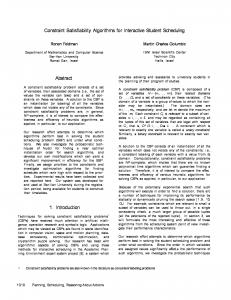
2.1.1 SAT Solvers. Given a propositional formula on a set of Boolean variables, a SAT solver determines if there exists an assignment of the variables such that the formula evaluates to true, or proves that no such assignment exists. SAT solvers are used in many applications as the lowest-level building block for reasoning tasks. Traditionally, SAT solvers only deal with Boolean propositional logic, though recently researchers started to look into possibilities of combining richer logics into the SAT solver framework. A D

E

B

C

Fig. 1.

A graph.

To give a very concrete, although simplistic, example of the syntax of problems solved by SAT solvers, consider a 3-colouring problem. It can be expressed as follows: for each vertex (e.g., for A) we introduce 3 Boolean variables (A1 , A2 , A3 ), which will be true if colour 1, 2 or 3 is assigned to the vertex. A basic constraint is that each vertex must be assigned exactly one colour, which we decompose into propositions meaning that “at least one colour is assigned to the vertex” and “the vertex cannot have two colours”. For A this gives: A1 ∨ A2 ∨ A3

¬A1 ∨ ¬A2

¬A2 ∨ ¬A3

¬A3 ∨ ¬A1

And similarly for B, C, D and E. The constraints we have used are clauses, i.e., disjunctions of literals, where a literal is a variable or its negation. Most SAT solvers take problem inputs in the so-called CNF (Conjunctive Normal Form) format as input, which means that the constraints have to be a conjunction of clauses. The remaining clauses for this problem state that each edge forces us to assign different colours to its extremities: ¬A1 ∨ ¬B1

¬A2 ∨ ¬B2

¬A3 ∨ ¬B3 . . .

15 variables and 4 × 5 + 7 × 3 = 41 clauses are needed to express this problem. SAT is quite a low-level language, but in practice the formulae are indeed typically generated from the automatic translation of a problem instead of hand-written. More precisely, there are in general two ways to use a SAT solver in an application. The simplest way is for the application to generate a Boolean formula and ask a SAT solver to determine the satisfiability of the formula. This approach is often referred to as the “eager approach” [Bryant et al. 2002]. Alternatively, the application can ACM Computing Surveys, Vol. 38, No. 4, December 2006.

6

·


reduce a problem into a series of related SAT queries that are incrementally solved by the SAT. Subsequent SAT queries are dynamically generated based on the results of previous queries. This approach is sometimes called the “lazy approach” [Barrett et al. 2002]. 2.1.2 Constraint Programming. Constraint Programming typically provides languages [Colmerauer 1990; Van Hentenryck 1989] or libraries [Puget 1994; Hamadi 2003] whose aim is to allow the development of application-specific search algorithms. This usually allows the rapid development of the optimisation/satisfaction part of larger applications. Because libraries (for instance C++ libraries like [Puget 1994; Hamadi 2003]) make it especially easy to integrate the constraint solving component into a larger application, this solution is typically the most widely accepted in the industry. For the sake of concreteness, and although the way to express problems in CP is in general dependent on the tool which is used, we also give an idea of how a graph colouring problem can be modelled as a Constraint Satisfaction Problem (or CSP1 ). Typically we would model the problem using variables ranging over a finite domain, which we can express as: A ∈ {1, 2, 3}, . . . Constraints are then imposed to enforce a dis-equality for each edge of the graph. All solvers provide slightly different constraint languages, but typically the difference constraint would be directly available, and we would be able to state: A 6= B, B 6= C, C 6= D, A 6= C, B 6= D, D 6= A, D 6= E Some solvers also provide higher-level constraints, allowing for instance to directly state that all variables in a list are pairwise different, using a statement of the kind alldiff([A, B, C, D]) instead of the first six constraints. The CP tool would typically be embedded in an application and the constraints would be processed, using the host programming language, from the data of the problem at hand. For instance, a loop would usually be used to generate a disequality constraint for each edge of the graph. In other words the graph-colouring part of the application can be developed using the CP tool instead of redeveloping an ad-hoc algorithm, but the integration with the rest of the application is transparent since the constraint solving facilities are called programmatically. 2.2

Typical Areas of Applications

2.2.1 Application Areas of SAT. SAT solvers have been used as a target language for many applications related to theorem proving, verification, Artificial In1 The

term CSP is often used in the literature to denote constraints expressed in an intentional way (table of allowed/forbidden tuples), and many papers even implicitly use the term CSP with the more specific meaning of binary intentional CSP in mind. In this survey these restrictions will not be assumed unless otherwise stated. To completely clarify the terminology, let us also note that there is a clear distinction between CP and CSP since CP refers, more broadly, to the whole approach of constrained-based problem modelling and solving. It covers some aspects, like the Constraint Programming languages, while the CSP literature focuses solely on the algorithms for solving CSPs. ACM Computing Surveys, Vol. 38, No. 4, December 2006.


·

7

telligence (AI) and Electronic Design Automation (EDA). Examples include AI planning [Kautz and Selman 1992], model checking [Clarke et al. 2001], automatic test pattern generation for circuits [Larrabee 1992] and decision procedures for various subsets of first order logics [Bryant et al. 2002; Barrett et al. 2002; Flanagan et al. 2003]. One of the most successful applications for SAT is verification and testing of digital systems [Prasad et al. 2005]. Techniques such as bounded model checking [Biere et al. 1999] have been widely adopted by the Integrated Circuits industry to test and verify the correctness of complicated designs. Many of these techniques use a SAT solver as the underlying reasoning engine because the verification is mostly carried out at the level of Boolean logic gates. More recently, researchers begin to study the problem of verifying digital systems at higher abstraction levels in order to verify more complicated properties and larger systems. Examples of such verification tasks include checking certain properties of programs and verifying the functional correctness of microprocessors [Burch and Dill 1994]. In these applications, systems are often described in rich logics. Translating these logics down to Boolean often causes significant overhead. Therefore, decision procedures for richer logic are often needed. SAT plays an important role in many of these decision procedures as the Boolean reasoning engine that glues other reasoning procedures together. This approach, sometimes called Satisfiability Modulo Theories (SMT), is an active research subject recently [Ranise and Tinelli 2003; Nieuwenhuis and Oliveras 2005; Barrett et al. 2005]. CP solvers can be regarded as a class of decision procedures with an ad-hoc way of combining theories.

2.2.2 Application Areas of CP. New applications of Constraint Programming appear every year; currently the most successful ones are found in configuration, scheduling, timetabling and resource allocation, which are of critical interest to many areas of activity such as manufacturing, transportation, logistics, financial services, utilities, energy, telecommunications, defense, retail, etc. Remarkably, before the wide adoption of SAT for verification and testing, early CP works addressed these problems [Simonis and Dincbas 1987; Graf et al. 1989]. Recently, there was a renewal of interest for CP in this area [Delzanno and Podelski 2001; Collavizza and Rueher 2006].

2.2.3 Synthesis. SAT and CP are two approaches to constraint satisfaction which differ in their philosophy and in their applications. As we shall see in subsequent sections, the importance of the applications of SAT for hardware and (more recently) software verification had some impact on the types of algorithms employed. For instance, complete solvers are preferable for this type of applications (see Sec. 4). The applications of CP to scheduling and similar industrial problems, on the other hand, had some impact on the philosophy underlying these tools: the CP community wanted tools that allow programming application-specific search strategies and integrating them into large applications. ACM Computing Surveys, Vol. 38, No. 4, December 2006.

8

3.

·


EXPRESSING PROBLEMS IN SAT AND CP

The philosophy adopted by CP tools could be summarised as “provide means to directly express all useful constraints”. On the contrary, the SAT approach is minimalistic. It typically provides a unique type of constraints (clauses) which is just expressive enough to state complex problems, although usually in a less direct way. Once the problem is modelled by a set of variables and constraints, the philosophies differ again in the way the user interacts with the solver: the SAT approach is essentially a black box approach in which no interaction is required – the solver is expected to find a solution without external tuning. The CP approach, on the contrary, provides the user with high-level tools so that she can express problem-specific knowledge and “program” the best algorithm for her application. 3.1

Modelling

3.1.1 Modelling Problems in SAT. The main challenge when using a SAT solver is to model the problem as a Boolean propositional formula. This modelling process (sometimes called encoding or translation) is studied by many researchers. Different applications require different translation techniques. In the past, people have been able to translate diverse problems such as AI planning [Kautz and Selman 1992], model checking [Biere et al. 1999], automatic test pattern generation (ATPG) for circuits [Larrabee 1992] and decision problems for various subsets of first order logics [Bryant et al. 2002] into SAT problems. For a given problem, different encoding techniques may produce formulae with very different performance characteristics for SAT solver. For example, many techniques have been proposed to efficiently translate logic equivalence with uninterpreted functions and separation logic into SAT [Strichman et al. 2002; Bryant et al. 2002; Seshia et al. 2003]. Input. Most often, the input to a SAT solver is a Boolean propositional formula in Conjunctive Normal Form (CNF). A CNF formula is a conjunction (logic and) of one or more clauses, each of which is a disjunction (logic or) of one or more literals. A literal is either a positive or a negative instance of a variable. Any (Boolean propositional) formula can be transformed into a equi-satisfiable CNF formula in linear time by introducing auxiliary variables [Tseitin 1968]. Non-clausal SAT solvers have been studied recently in the SAT community and shown to be at least as efficient as clausal SAT solvers [Thiffault et al. 2004]. This fact is also known in the EDA (Electronic Design Automation) community, which traditionally focus on reasoning with logic circuits [Ganai et al. 2002]. Output. Traditionally, given a SAT instance, a SAT solver only needs to answer true or false depending on the satisfiability of the formula. If the instance is satisfiable, most SAT solvers can also output a satisfying assignment (a model) of the instance. Sometimes the applications prefer the solution to have certain properties. For example, applications such as explicating theorem provers [Flanagan et al. 2003] may prefer solutions to contain only a small subset of the involved variables (cf. Sec. 8.1). For unsatisfiable instances, some applications may want the SAT solvers to produce a subset of the original clauses that is unsatisfiable by itself (i.e., an unsatisfiable core). Some algorithms have been proposed to achieve this [Zhang and Malik 2003b; Oh et al. 2004a]. ACM Computing Surveys, Vol. 38, No. 4, December 2006.


·

9

One advantage of the very simple representation language used by SAT solvers is that all the effort can be focused on a single representation. This resulted in highly optimised datastructures and efficient implementations of the reasoning on this representation, as we will see in later sections2 . 3.1.2 Modelling Problems in CP. A first step in problem solving with the CP approach is to specify the problem by defining its (variables and) constraints. When using CLP or libraries like Ilog Solver or Disolver, one uses the facilities of the host language (Prolog or C++) to do that. Constraint Programming tools provide a rich set of constraints that are designed to express the relations between the variables of the problem in the most direct way possible. For instance, constraints are directly available to express numerical relations (e.g., 2x + y = z), constraints on basic data structures like arrays (e.g., t[x] = y, where variables t, x and y represent, respectively, an array, an index, and a value), or higher-level constraints with a more complex meaning (e.g., a constraint on a set of variables {xi | i ∈ 1..n} imposing that ∀i ∀j > i. xi 6= xj ). More generally, an important strength of the constraint programming framework comes from its flexibility. Constraint Programming environments provide users with a library of constraints that helps them state their problems in the most direct way. Constraints can be understood under 3 directions: —Logical: the semantics of a constraint can be defined in a simple, declarative way: a constraint is defined by the combinations of values it accepts for the variables it relates (for instance the constraint x < y will be satisfied by any solution which assigns a larger value to y than to x). —Deductive: the way the constraint interacts with the solver is by informing it of deductions it makes in reaction to events and decisions arising during the search process (for instance a constraint x < y will react to the event x > 5 by deducing y > 6). —Algorithmic: there are many ways to implement the deduction rules of complex constraints, and the role of the providers of the CP toolkit is to make sure the best efficiency is obtained. More details on constraint propagation are given in Sec. 6. We now describe some of the constraints that most CP tools provide. Numerical Constraints. Numerical data are ubiquitous in most applications, and numerical constraints are natively integrated in most CP environments. 2 CNF

formulae in a SAT solver are usually stored in a linear way, sometimes called a sparse matrix representation. The data set can be regarded as a sparse matrix with variables as columns and clauses as rows. In a sparse matrix representation, the literals of each clause occupy their own space and no overlap exists between clauses. Various techniques have been proposed to make such a representation space efficient and cache friendly (e.g., by allocating a continuous memory pool for the clause database) and to perform periodical garbage collection and data set compaction. Other representations for a CNF clause database exist. For example, data structures such as tries [Zhang and Stickel 2000] and ZBDDs [Chatalic and Simon 2001] have been proposed to compress the data size by allowing sharing between clauses. These techniques are proven to be too costly for search based SAT solvers, but have found applications in resolution based solvers. ACM Computing Surveys, Vol. 38, No. 4, December 2006.

10

·


In most applications, the numerical constraints that naturally occur are linear, e.g., the primitive operations are addition and multiplication by a constant. For pure integer programming3 problems [Chvatal 1983; Wolsey 1998], a vast literature of mathematical programming is available and very efficient, specialised solvers exist. Indeed, a whole area of research in Constraint Programming concerns the integration of CP and Integer Programming methods [Milano 2004]. While CP tools do not usually compete with Integer Programming solvers for pure linear constraints, they have the advantage of being more flexible and effective at solving problems with other types of constraints as well. Because numerical domains can be very large, most CP tools rely on intervals to represent the range of variables that are subject to numerical constraints, and use interval propagation (cf. Sec. 5.2) for reasoning on these constraints.. Symbolic Constraints and Meta-constraints. A wide range of constraints which are not easily representable in SAT can be integrated to CP architectures. Highlevel constraints can for instance be defined on lists or data structures. These are often referred to as symbolic constraints since they allow the definition of constraints between data that are neither numerical nor Boolean4 . For instance, one can define constraints imposing t[x] = y, where x is an integer-valued unknown variable, t is an array of unknown variables, and y is another variable. The CP framework is also flexible enough to allow users to specify problems with arbitrary Boolean combinations of constraints – not only conjunctions of constraints [Van Hentenryck and Deville 1991]. Such constraints are typically called metaconstraints. Disjunctions of constraints are common in some applications, and implications can be used, typically, to put constraints conditionally. It is indeed possible to decompose any combination of constraints into a conjunction provided reified versions of the constraints are available: a reified version of a constraint (say constraint x − y = z) is a constraint with an additional parameter, whose domain is Boolean, and which is true iff the constraint holds. For instance we would have a constraint for (x − y = z) ↔ b and the distance constraint x − y = 5 ∨ y − x = 5 is seen by the solver as the conjunction (x − y = 5) ↔ a, (y − x) = 5 ↔ b, a ∨ b. A number of proposals have been made to improve the way Boolean combinations of constraints are handled [Bacchus and Walsh 2005]. For instance disjunction should ideally be propagated in a constructive way, i.e., the solver should be able to infer information before knowing which constraint actually holds. The implication connector can have different effects in CP tools, for instance the blocking implication used in the language CC(FD) [Van Hentenryck et al. 1998] puts a constraint (right3 In this survey we focus on problems whose variables range over discrete domains (enumerated types or integers). Specialised techniques, like the Simplex algorithm, can be applied to problem of computing real-valued solutions to linear constraints [Chvatal 1983], which is computationally much easier (polynomial time complexity). 4 Pioneering works in Constraint Logic Programming used to consider constraints on many different domains, like Booleans, integers, rationals, real numbers, strings, lists, trees or records (“feature structures”), and the CLP(X) framework was parametrised by the domain (X) of computation [Jaffar and Lassez 1987]. In a sense, logic programming, in which CP has some of its roots, intensively uses a particular form of constraints since its unification mechanism [Robinson 1965] resolves equalities over terms. The expression of unification as a constraint solving mechanism by [Colmerauer 1984] paved the way for Constraint Logic Programming.



·

11

hand side) only if another constraint (left-hand side, or guard) is entailed by the constraint store. This operational semantics allows to use it as a programming construct. Global Constraints. For some application areas of CP like scheduling, it is possible to identify complex constraints that are frequently used. Such constraints can typically be expressed using a conjunction of primitive numerical and logical constraints, but using specialised algorithms it is in general possible to make stronger deductions on these constraints, and to make these deductions more efficiently. Such high-level constraints are called global constraints [Beldiceanu and Contejean 1994; Régin 1994]. Some CP libraries provide a very rich set of global constraints (dozens of them for the largest libraries), and a good use of these components can allow experts to obtain models with highly improved performances. Among the best-known global constraints, let us mention: —The alldiff constraint: imposed on a list of variables, it constraints their values to be all different (i.e., the constraint can be expressed as ∀i ∀j > i. xi 6= xj ). —Constraints on lists, which ensure that the elements are sorted, or impose the membership of certain elements or bound the cardinality of the elements, [Van Hentenryck and Deville 1991], etc. —Application-specific constraints, like the cumulative constraint, used in planning/scheduling applications. This constraint expresses a complex logical statement whose meaning is intuitively: “the sum of the quantities of resource r needed by all tasks active at any instant is never more than the available capacity”. Historically the introduction of global constraints was an important step that allowed CP to be used for real-world applications. As a means to integrate specialised algorithms from operations research and graph theory into the CP framework, they are often unavoidable in the resolution of complex problems. The reason why they are critical in terms of efficiency is easily understood if one considers perhaps the most emblematic of them: the alldiff constraint. The alldiff constraint can indeed make an exponential difference because it provides specialised algorithms for problems on which branch and prune is inadequate and takes exponential time. Take for instance alldiff([x1 . . . xn ]) where each xi ranges over 1..n-1. This problem, which encodes the Pigeon Hole Principle, is unsatisfiable. Deduction techniques classically used in constraint solvers are not very effective when the difference constraints are considered independently of each other, and a classical search algorithm which does not use global information on the group of disequalities will entirely explore a search tree of size (n−1)! to prove inconsistency5 (in fact, the runtime will be exponential with any resolution-based technique, including search, propagation and learning [Mitchell 1998]). It is well-known that search-based (and resolution-based) solvers have intrinsic limitations, and global constraints have been a means, in the CP world, to overcome them – for instance all difference constraints can be propagated very efficiently using graph-based algorithms (see [Régin 1994] and Sec. 6.2.3). 5 On

this example a simple check that the union of the possible values for the xi s is always of cardinality greater than or equal to n would also easily detect the inconsistency. ACM Computing Surveys, Vol. 38, No. 4, December 2006.

12

·


We refer the reader to [Beldiceanu et al. 2005] for a complete catalog of global constraints. Note that this reference, which is more than 1300 pages long, presents a list of about 235 constraints. This shows that the literature on global constraints is rich, but that a high expertise is also needed to use these constraints effectively. Modelling Languages. Constraint Programming provides a rich number of features that allow the user to express complex problems in a direct and declarative way. Additionally, some research has focused on the design of declarative modelling languages that provide a high-level algebraic or logical syntax to express the constraints of the problem. Typical Pconstructs provided by these languages are arrays, loops or forall quantification, i notation for sums, etc. The way constraints are extracted from the declarative syntax is usually straightforward. There seems to be room for static analysis and program optimisation, but this research area is currently at a preliminary stage [Frisch et al. 2005; Cadoli and Mancini 2006]. An example of state-of-the-art modelling language is OPL [Van Hentenryck and Michel 2002], which is inspired from mathematical programming languages like AMPL [Fourer et al. 1993] and also has roots in AI work of the 70s [Laurière 1978]. This language allows to separate between the specification of the problem (e.g., graph colouring, or a resource allocation problem) and the data of a particular instance (the graph, or matrices with costs, etc). This decoupling allows a better reusability of the specifications. 3.1.3 Synthesis. The features provided by SAT and CP w.r.t. modelling differ greatly and are due to a different philosophy. SAT solvers do not aim at being directly used to express a problem by hand; instead they are used as a target language by higher-level reasoning tools that automatically translate other problems or formalisms into CNF formulae. CP, on the other hand, is directly used to express problems and the solver is designed to be called directly from the application in which the constraint solving part is embedded. Impact of the Model on the Performances. Common to SAT and CP is the issue of finding a good model for the problem at hand. Once a model is chosen, expressing it using the SAT/CP tool is usually relatively easy, but problems can usually be formulated in a variety of ways that are not equally easy to solve. It is more an art than a science to decide which model should be preferred. In SAT, the modelling process (sometimes called encoding or translation) has been studied by many authors. Some problems are known to have very different behaviours for different SAT translations [Seshia et al. 2003; Nam et al. 2004]. Special translation algorithms have been proposed to handle constraints with certain structures (e.g., [Ganai et al. 2004; Velev 2004]). There are many similarities between the encoding of problems expressed in rich logics into Boolean propositional formulae and the compilation of a higher level programming language into machine code. It was observed that, in certain applications, some of the commonly used techniques in compiler optimisation, such as loop unrolling and constant propagation, can also be applied to SAT encoding [Marinov et al. 2005]. In CP, the good use of global constraints and other modelling choices is of critical importance to the resolution speed. One can often greatly improve the performance of the solver by reformulating the problem. Typical reformulation techniques are ACM Computing Surveys, Vol. 38, No. 4, December 2006.


·

13

to try alternative models, to add redundant constraints, to break the symmetries of the problem with additional constraints [Gent and Smith 2000], or even to combine different models of the same problem and link them together via so-called “channeling constraints”, which propagate information between the variables of different representations [Smith 2002]. Because of the wider choice of constraints they provide, the performance of CP tools is usually (even) more dependent on modelling issues than in the case of SAT tools. One design choice in SAT solvers is to have all features fully automated. For instance, in most of the work done on symmetries is SAT, the detection of symmetries is performed by the solver [Aloul et al. 2003], while in early CP work the user was usually expected to express them explicitly. Both approaches have their pros and cons. It has been argued by some researchers, even inside the CP community, that the expertise needed by CP tools is a major obstacle limiting their widespread use in the industry [Puget 2004]. An important challenge in CP is to assist or automate the modelling issues (note that these issues are also tightly related to the discussion on the programming features of SAT and CP, see Sec. 3.2). On the other hand, some techniques available in CP have not found their way to SAT solvers simply because they cannot be fully automated. For instance, to the best of our knowledge, channeling constraints have not been studied in SAT. Handling Numerical Data. An important question driving the choice between SAT and CP technologies for a particular application is whether numerics will intensively be used. Arithmetics is natively supported by CP tools while in SAT they need to be converted into Boolean logic. There are several ways of encoding a numerical variable x into SAT. The simplest way is to create one Boolean variable Bi for each possible value i of the variable x; Bi will be true iff x = i, and some constraints need to be added to impose that exactly one of the Bi s is true. A more compact method, called the logarithmic encoding, considers a vector of Boolean variables hB0 . . . Bn i as the binary encoding of a number ranging over [0, 2n ]; this encoding is more appropriate when the constraints represent arithmetic operations on large numbers, for instance the addition of two 64-bit integers (note that the Boolean constraints used for this encoding directly reflect the circuit of the operation, for instance a 64-bit adder). Surprisingly, encodings of numbers in SAT have been successfully used in verification problems [Seshia and Bryant 2004], so it would be na¨ıve to conclude that SAT solvers cannot cope with numbers at all. The use of incremental encodings can in particular compensate the problem of the size of encoding. However, these encodings are not direct and are complex to implement, and SAT solvers do not exploit the arithmetic operations supported natively by the processor. On the contrary, CP tools can provide direct support for numerical constraints and the internal representation of these constraints is typically space-effective (typically intervals). Awareness of Problem Structure. Problem representation in SAT is flat and homogeneous, and there is little room for giving the solver information on the structure of the problem. Even if the formulation of a problem naturally exhibits particular graph-theoretic properties or high-level features, this is lost during the encoding into Boolean logic. To alleviate this problem, some authors tried to incorporate the ACM Computing Surveys, Vol. 38, No. 4, December 2006.

14

·


structure information of the original problem as hints to guide the SAT search, for example, by exploiting the signal correlations of circuits [Lu et al. 2003] or structure similarities between different time-frames of the same sequential circuit [Strichman 1999], or make the SAT solver aware of the structural symmetry [Sabharwal 2005]. On the contrary, CP provides rich tools for the expression of the structure of the problems at hand - at the cost of being more difficult to learn and to require more expertise. One tool to express problem semantic in CP is the use of global constraints. An example of using special reasoning technique in SAT is equivalence reasoning. To express an equivalence class with n variables, 2n−1 clauses, each with n literals, are needed. It is well known that reasoning on equivalence is exponential for resolution based SAT solvers. Search is just a special case of guided resolution. Therefore, traditional SAT solvers, even combined with learning, will stall on problems that contain many equivalences. There is some work on incorporating equivalence reasoning into SAT solvers in the literature [Li 2000; Dixon et al. 2004]. Other works aim at recovering structural information from the SAT instance using preprocessing or graph analysis, which allows to restate the problem in a more concise way so that some equality reduction can be performed [Bacchus and Winter 2003]. The main reason why SAT solvers are not very structure-aware is that the CNF format is very low-level, but note that this choice also has great advantages. SAT solvers are highly optimised to perform efficient deduction on CNF Boolean formulae. CNF can be compactly stored in memory with very good cache behaviour. Highly efficient deduction algorithms have been proposed to perform reasoning on clause. Many branching heuristics and conflict-driven learning techniques also rely on the fact that the formula is in CNF. By combining these techniques, modern SAT solvers routinely solve instances with tens of thousands of variables and hundreds of thousands of clauses. Versatility. SAT solvers are highly specialised in doing one thing – Boolean satisfiability, while CP tools provide a more general framework in which additional features can be plugged. On the other hand, the simplicity of use of SAT solvers, which have a clear interface with a simple and uniform representation language, makes it easier to learn and use for non-specialists. (See also Sec. 4.4 on integration of SAT/CP algorithms for more details.) 3.2

Programming

3.2.1 Tuning of SAT Solvers. Given a SAT instance, usually a SAT solver will try to find a solution or to prove the unsatisfiability without any interference from the caller. There are many reasons for regarding SAT solvers as black-boxes. First of all, through many years of research, a number of good heuristics have been developed that seem to be efficient for many classes of problems generated from real world applications. A large number of SAT test benchmarks exists in the public domain. A newly proposed heuristic usually has to work well on most of them in order to be considered a good heuristic. When a real problem is reduced to a SAT instance, much of its internal structure is lost in the translation phase. Therefore, intuition obtained from the problem domain may not help much on solving the resulting SAT formula. For example, it is known that branching heuristics based on ACM Computing Surveys, Vol. 38, No. 4, December 2006.


·

15

variable dependencies do not work very well even though there is a strong intuition behind such heuristics [Giunchiglia et al. 2002]. Still, there are works that exploit domain specific knowledge to help prune search spaces. For example, signal correlation between nodes of a Boolean circuit can be used to derive good branching and learning heuristics for equivalence checking of logic circuits [Lu et al. 2003]. 3.2.2 Programming a Search Strategy in CP. The constraints obtained from the modelling can in theory be solved directly, and CP solvers have default strategies which can be applied in the absence of user-defined instructions. But CP tools typically fail to achieve the best performances without some application-specific tuning. A typical parameter which has to be carefully tuned by the user to obtain the best performance is the order in which the variables have to be instantiated during the search. For many applications, variables divide into groups that have different meanings, and some variables play a more important role. This is often obvious to the expert – but not necessarily to the automated procedure. This tuning can either be achieved by providing a list of variables to start with or by selecting one of a number of predefined enumeration strategies (e.g., by increasing domain size, see Sec. 5.1 on branching). In some libraries, it is even possible to specify alternative choices of algorithms, like local search or stronger propagation methods. In many Constraint Programming tools, the tuning is essentially done by giving well-chosen parameters to the solver. Some other tools provide higher-level ways of expressing strategies, which culminate with full-fledged, declarative languages. For instance, in OPL, one can construct a search strategy using advanced constructs [Van Hentenryck et al. 2000] for nondeterministic choice and ordering as well as event-driven conditions. The idea of languages dedicated to search procedures dates back to the 1970s [Fikes 1970] and seems to be increasingly present in recent languages [Van Hentenryck and Michel 2002]. 3.2.3 Synthesis. The philosophy of SAT regarding the algorithmic problem solving is in general to let the solver find the best way to deal with the instance at hand. CP, on the other hand, typically provides a wide range of methods to solve the problem, so that the best one can be hand picked. Once again, both choices have pros and cons: SAT is used as a target language which is low-level, so that many reasoning tasks can be compiled to it using some translation scripts. Because the language is low-level, it is not easy – nor desirable – to let the user specify variable-ordering strategies and other information. CP, on the other hand, aims at being used programmatically, with queries directly coming from another application. This gives the programmer opportunities to inform the solver with helpful, application-specific information, and to choose the best solving functions provided by the library. On the other hand, the expertise required is higher, which limits the use of this technology by non-experts. 4. 4.1

ALGORITHMS FOR SAT AND CP Complete v. Incomplete Algorithms

A large range of techniques have been proposed to solve constraint satisfaction and optimisation problems over the years. Some of these methods arose from fields as ACM Computing Surveys, Vol. 38, No. 4, December 2006.

16

·


diverse as mathematical programming (dynamic programming [Bellman 1957], linear relaxations and cutting plane generations for integer linear constraints [Wolsey 1998], which use simplex and interior point methods from Linear Programming [Chvatal 1983]), or statistical physics [Mézard and Zecchina 2002], not to mention some attempts in using non-conventional computational paradigms like DNA computing [Dantsin and Wolpert 2002]. Giving a complete overview of all the approaches that have been considered would require considerable space and the authors of this survey lack the required authority on some of these areas. Still, the most robust, state-of-the-art solvers typically rely on a small number of established techniques that sometimes date back to the early 60s [Davis and Putnam 1960; Davis et al. 1962]. One can roughly distinguish between the following two categories of constraint solving methods: —Incomplete methods aim at finding solutions by heuristics means, without exhaustively exploring the search space. These methods are typically unable to detect that no solution exists. When no solution is generated after some time limit, one cannot tell whether existing solutions were missed or whether the problem is indeed unsatisfiable6 . Most of incomplete methods are stochastic, i.e., they use random moves. —Complete methods aim at exploring the entire solution space, typically using backtrack search (see Sec. 5 and 7). Since the exhaustive enumeration of the points in the search space would be too costly, pruning techniques are typically used to rapidly determine that certain regions contain no solution. (Sec. 6 will present pruning methods in more details, in particular propagation methods.) The rest of Sec. 4 will give a brief overview of incomplete and complete methods, trying to emphasise the similarities and differences between the ways these techniques are used in SAT and CP. Sec. 5, 6 and 7 will then go into a more detailed comparison of a class of complete algorithms which are of particular importance: branch & prune methods. 4.2

A Brief Overview of Incomplete Methods

A wide range of incomplete methods have been proposed to solve constraint satisfaction and optimisation problems. These methods can roughly be divided into population-based algorithms and other local search methods. —Population-based algorithms maintain a population of individuals which typically correspond to points of the search space. This population is iteratively modified and the goal is to ultimately find an individual that satisfies all the constraints, or one that is of high quality w.r.t. the objective function of the problem. One way to update the population is to use genetic algorithms, with operations like cross-over and mutation, to obtain new individuals from the existing population (see [Michalewicz 1995] for a survey of evolutionary computation methods that is essentially restricted to nonlinear constraints). Other population-based methods 6 Some algorithms, including some stochastic ones, are nevertheless Probabilistically Asymptotically Complete [Hoos 1999], which means that they offer a probabilistic guarantee that all the search space will eventually be explored.



·

17

have been proposed, for instance ant colony optimisation [Dorigo and Stutzle 2004] and other “swarm-based” algorithms, which are inspired by the way ants or other social animals solve complex problems using collective intelligence and stygmergy, i.e., indirect communication via pheromone laying. —Other (non population-based) incomplete methods typically consider a unique point at every time step. The goal is, here again, to reach a (possibly optimal) solution by exploring the neighbourhood of the current point and moving it stochastically along the search space. Well-known representatives of the stochastic local search (SLS, a.k.a. “hill-climbing”) family are simulated annealing [Kirkpatrick et al. 1983] and Tabu search [Glover and Laguna 1995]. A recent general reference on the topic is [Hoos and Stutzle 2004]. Common to all stochastic local search methods is a small number of basic, wellidentified principles, of which many instantiations have been proposed along the years. SLS algorithms use intensification to explore the close neighbourhood of the current point; on the other hand they need a source of diversification to avoid getting stuck in a neighbourhood in which no (globally optimal) solution can be found. The diversification component is usually the most difficult to define. A typical technique is to allow with a non-zero probability to make moves that do not seem a priori promising; this allows the algorithm to explore parts of the search space that it would otherwise never reach (“noise” strategies). While noise strategies allow some diversification in the choice of the moves, randomness can also be injected by directly applying random changes to the current point between some moves (“perturbation” approach). While deterministic variants exist, the incomplete methods used in practice are typically stochastic, and rely on (pseudo-)random generators. This feature typically improves their robustness, but one drawback is that it makes the tuning of these algorithms particularly tiresome. Local search techniques are typically parametrised by a large number of numerical constants that determine the probability of applying perturbations, the number of steps to wait before applying the diversification technique, etc. Finding good choices for these parameters is critical to obtain good performance. 4.2.1 Incomplete Methods in SAT. Incomplete methods based on stochastic local search started to have considerable success on SAT in the 1990s with the introduction of GSAT [Selman et al. 1992], which showed that local search based on the objective of maximising the number of satisfied clauses could be used to solve large satisfiability problems. Its followers like WalkSAT [Selman et al. 1994] could deal with instances unsolvable using complete solvers. However, complete SAT solvers have recently seen considerable improvements due to the invention of learning and non-chronological backtracking techniques [Marques-Silva and Sakallah 1996; Bayardo and Schrag 1997] and the introduction of well designed solvers such as Chaff [Moskewicz et al. 2001]. Modern complete SAT solvers are especially competitive when the instances are generated from real-world applications (i.e., exhibits some structure). Moreover, the most important recent applications of SAT is verification, where complete solvers are preferable. Therefore, complete SAT solvers are attracting most of the attention in recent years. Still, great progress has been made on ACM Computing Surveys, Vol. 38, No. 4, December 2006.

18

·


DPLL() { status = preprocess(); if (status != UNKNOWN) return status; while(true) { make_branch_decision(); while (true) { status = deduce(); if (status == INCONSISTENT) { resolved = analyse_conflict_and_backtrack(); if (!resolved) return UNSATISFIABLE; } else if (status == SOLUTION_FOUND) return SATISFIABLE; else break; } } } }

Fig. 2.

The iterative description of DPLL.

local search SAT solvers. An example of a state-of-the-art stochastic SAT solver is a system called SAPS [Hutter et al. 2002]; its heuristic is based on weights, assigned to each clause of the CNF, which are updated using scaling and smoothing steps. 4.2.2 Incomplete Methods in CP. The use of local search integrated with Constraint Programming, (see, e.g., [Pesant and Gendreau 1999]), or as an alternative framework for constraint solving and optimisation (e.g., [Davenport et al. 1994]) has been considered since the early days of CP. An important difference with SAT is that many applications of Constraint Programming deal with optimisation problems, for which incomplete approaches based on local search are effective at finding good solutions, and exhaustive search is indeed often infeasible. An example of recent Constraint Programming approach to incomplete methods is the Comet system, which proposes a high-level language to program local search algorithms [Van Hentenryck and Michel 2005]. 4.3

A Brief Overview of Complete Algorithms

The complete algorithms proposed for SAT and CP are also quite numerous. Most complete algorithms are based on backtrack search. In these approaches, a search tree is built/explored and some local reasoning is used at each node to prune away certain branches. An alternative search algorithm used in SAT is proposed by St˚ almarck [Sheeran and St˚ almarck 2000], which use breadth-first search among other techniques. The main approaches in SAT other than search are resolution (see Sec. 6.1.1), which iteratively builds all the clauses implied by the problem until unsatisfiability is detected, and algorithms based on data structures to represent the entire set of solutions of the problems. These data structures are typically variants of binary decision diagrams [Bryant 1986]. 4.3.1 Complete Methods in SAT. The backtrack algorithm is most often attributed to Davis, Putnam, Logemann and Loveland (DPLL) [Davis and Putnam ACM Computing Surveys, Vol. 38, No. 4, December 2006.


·

19

1960; Davis et al. 1962]7 . The original paper described a recursive algorithm but, in practice, most solvers implement the algorithm as an iterative procedure. The pseudo-code based on the branch and prune principle is described in Fig. 2. There are three essential constituents of backtracking algorithms: the heuristics to choose variables for branching (function make branch decision), the algorithm used for pruning and reasoning (function deduce), and the algorithm to handle conflicts when they occur (function analyse conflict and backtrack). These three parts will be discussed in Sec. 5, 6 and 7, respectively. The preprocess step can be regarded as an extra deduction step to simplify the problem before any branch is made. Since it is only carried out once, the preprocessor can employ some more powerful but more expensive reasoning mechanisms than the regular deduce function in order to simplify the problem as much as possible. We will briefly overview some of the preprocessing algorithms in Sec. 6. 4.3.2 Complete Methods in CP. If we exclude the historical generate and test algorithm which completely generates an assignment of the problem variables before testing the associated constraints, the most prominent algorithm is backtrack search [Golomb and Baumert 65]. Today, the backtrack search algorithms used in CP are close to the ones used in SAT (at least at the conceptual level). They define a search tree by dynamically selecting a value for a variable. This is called a branching decision. Each decision is propagated through the underlying constraint engine. When an inconsistency is detected by the engine, it can be analysed to perform (possibly non-chronological) backtracking. If alternatives values are available, the consequences of the inconsistency are propagated through a process called refutation. The engine may add a new constraint which records the negation of the previous attempt (no-good learning). It has been observed that the initial choices in a tree search are by far the most critical. One mistake at a very early level can result in a very expensive and deep unfruitful systematic exploration. To overcome this problem the initial backtracking algorithm has been revisited by many researchers [Harvey and Ginsberg 1995; Meseguer 1997; Gomes et al. 1998] (see Sec. 5). 4.4

Integration of Algorithms

Because a wide range of algorithms have been proposed for both SAT and Constraint Satisfaction Problems, an interesting thread of research has investigated the possibility to mix the algorithms available and combine their respective advantages. Additionally, it is sometimes needed to mix solvers of different types to tackle problems whose formulation requires a mix of several types of constraints, possibly on variables ranging over several domains (e.g., some real-valued, some discrete). We can distinguish between: —Cooperation, which is the integration of several algorithms that are run together on the same problem and exchange some information to make their resolution easier. 7 The

version of the algorithm which is currently used actually corresponds to the second version, i.e., the one by Davis, Logemann and Loveland. The term DPLL, however, is generally used. ACM Computing Surveys, Vol. 38, No. 4, December 2006.

20

·


—Hybridisation, which denotes the design of a new algorithm composed of features taken from algorithms of different categories (typically a complete solver that occasionally performs some steps of local search). —Combination, in which solvers for different types of problems are mixed, allowing to solve problems not solvable by any of them independently (e.g., mixed linear integer programming deals with problems with linear constraints on data that are partly real-valued, partly integer-valued.). Integration is used as a generic term for all methods which are based on one of these forms of mixing. In the context of SAT, some hybrid procedures were recently proposed. They combine stochastic algorithm with resolution, which guarantees completeness [Fang and Ruml 2004], or with search, which allows better performance on structured instances [Hirsch and Kojevnikov 2001]. The most common form of integration involving SAT solvers is otherwise combination. This is because SAT solvers are often used in applications that require to mix propositional reasoning with richer logic theories such as integer or real arithmetics, equivalences and uninterpreted function symbols, etc. Such combination-based decision procedures based on SAT are often called Satisfiability Modulo Theories (SMT) provers. Two well known methods to combine different theories are the Nelson-Oppen method [Nelson and Oppen 1979] and the Shostak method [Shostak 1984]. An appealing recent framework for SMT is the DPLL(T) framework [Nieuwenhuis and Oliveras 2005]. The Constraint Programming community, on the other hand, has traditionally been using all forms of solver integration, perhaps because a large number of established techniques from Operations Research naturally apply to some classical Constraint Programming applications. The connections between Constraint Programming and mathematical programming have therefore been widely studied [Hooker 2000; Milano 2004] and more general frameworks for solver cooperation have been proposed [Monfroy and Castro 2003]. 4.5

Synthesis

Both SAT and CP have benefited from a wide range of proposals defining complete and incomplete algorithms. The state-of-the-art algorithms for both areas are in many respects similar: stochastic local search usually appears as the leading class of incomplete solvers, while the best complete solvers are based on a backtrack search that essentially uses the same kind of propagation (unit propagation and arc-consistency, cf. Sec. 6.1 and 6.2, respectively). More details on the important class of branch & prune SAT/CP solvers will be given in the next sections: Sec. 5 will more specifically focus on branching while Sec. 6 will deal with the pruning part. A topic which shows more differences in the SAT and CP approaches concerns the conflict analysis techniques, which are the last important enhancement of branch & prune we consider, and which are discussed in Sec. 7. 5. 5.1

BRANCHING SAT Heuristics

In SAT, since only two choices are possible for each variable, usually variable selection is more important. The heuristics for choosing values are more or less arbiACM Computing Surveys, Vol. 38, No. 4, December 2006.


·

21

trary, usually based on some obvious statistics. In practice, most of the challenging SAT instances are unsatisfiable. The solver has to search the entire space one way or the other. Therefore, the main research focus on SAT branching heuristics is to discover conflicts as early as possible. Another principle guiding the design of branching heuristics in SAT is that they must be cheap to evaluate – a heuristic that would require iterating through all the clauses of the problem would clearly not be affordable on large instances. Currently the most successful branching heuristics all have sub-linear asymptotic time complexity with regard to the size of the formula. The decision heuristics used in the first generation of SAT solvers were mostly based on statistics on the formula. Early branching heuristics such as Bohm’s Heuristic (reported in [Buro and B¨ uning 1993]), Maximum Occurrences on Minimum sized clauses (MOM) (e.g., [Freeman 1995]), and Jeroslow-Wang [Jeroslow and Wang 1990] are greedy algorithms that either try to produce a large number of implications or to satisfy as many clauses as possible. These heuristics use some functions to estimate the effect of branching on each free variable, and choose the variable that has the maximum function value as the next branching variable. One of the most successful branching heuristics based on such statistics is introduced in the SAT solver GRASP [Marques-Silva 1999]. This scheme proposes the use of the counts of literals appearing in unresolved clauses, i.e., clauses which are not already true under the current partial assignment. In particular, it was found that the heuristic called DLIS gave quite good results for the benchmarks tested. DLIS chooses the variable with the Dynamic Largest Individual Sum of its literal count as the next decision variable. In the DLIS case, the counts are state-dependent in the sense that different variable assignments will give different counts for the same CNF formula because whether a clause is unresolved (unsatisfied) depends on the variable assignment. Because the counts are state-dependent, counts for all the free variables need to be recalculated at every branching point. This often introduces significant overhead. Moreover, the counts are static in the sense that they depend only on current state (i.e., variable assignments, original and learnt clauses, etc) of the solver. The heuristic is oblivious to the search process of the SAT solver (i.e., how the solver reaches the current state). Chaff [Moskewicz et al. 2001] proposed a branching heuristic called Variable State Independent Decaying Sum (VSIDS) that tried to eliminate both of the problems. VSIDS keeps a score for each of the two phases of a variable. Initially, the scores are the number of occurrences of the corresponding literals in the original CNF formula. Because of the learning mechanism (to be discussed in Sec. 7), additional clauses (and literals) are added to the clause database as the search progresses. VSIDS increases the score of a literal by a constant value whenever an added clause contains this literal. Moreover, as the search progresses, all the scores are periodically divided by a constant. In effect, the VSIDS score is a literal occurrence count with higher weight on the more recently added literals. VSIDS branches on the free literal with the highest score. Because scores in VSIDS are variable-state independent (i.e., unrelated to the current variable assignment), they are very cheap to maintain. In practice, profiling shows that branching usually takes less than ten percent of the total solving ACM Computing Surveys, Vol. 38, No. 4, December 2006.

22

·


time. In VSIDS, the scores are not static statistics. They take the search history into consideration. VSIDS tries to branch on variables that are “active recently”. The activity of a variable is captured by the score that is related to the literal’s occurrences. The focus on recent events is captured by decaying the scores periodically. Experimental results show that VSIDS is much more effective in solving real world instances compared with static branching heuristics. Recently, several new branching heuristics have been proposed that further push the ideas of VSIDS. For instance, Berkmin [Goldberg and Novikov 2002] proposed to take into account the scores of the literals that are involved in the generation of these clauses (in addition to the literals present in these clauses). Moreover, it proposed to choose to branch on a free literal that appears in the latest learnt clauses. Siege [Ryan 2004] proposed another branching scheme that heuristically moves literals that appear in the latest learnt clauses up to the front of the branching priority queue. Yet another heuristic [Dershowitz et al. 2005] moves active clauses to the front of a clause list and chooses to branch on literals occurring in an unresolved clause in front of the list. These algorithms are all different ways to capture the “active recently” principle. All of them seem to be quite competitive in performance compared with VSIDS. Almost all SAT solvers developed recently that are optimised for real world SAT instances employ a state independent dynamic decision heuristics. It is well known that bad choices in early branch variable selection can make the problem much harder to solve. Random restarts [Gomes et al. 1998] provide a heuristic that tries to alleviate this problem by periodically resetting the solver and starting search from the very beginning. In modern SAT solvers, after restart learnt clauses are usually carried over, only variable assignments are thrown away. This allows the solver to explore new solution spaces without wasting previous search effort. Restart is an important feature that has a huge impact on the robustness and efficiency of SAT solvers. Unsurprisingly, researchers have tried to tune restart strategies to make it more intelligent and less random [Kautz et al. 2002]. 5.2

CP Heuristics

5.2.1 Variable and Value Ordering. The general idea guiding variable and value selection is usually summarised under the “fail first” principle, which basically says that “to succeed, try first where you are most likely to fail”. The most common variable heuristics are: MINDOM (selects the variable with the smallest domain), MAXDEG (variable connected to the largest number of constraints), DOMDEG ([Bessière and Régin 1996], favours variables with small domains and large degrees), BRELAZ (MINDOM fail-first principle that breaks ties by returning the first variable connected to the largest number of unassigned variables in the constraint graph [Brelaz 1979]). Alternatively, the solver can simply consider variables according to a user-defined variable ordering (LEX). Classical value ordering heuristics include LEX (lexicographical ordering), INVLEX (reverse lexicographical ordering), MIDDLE (median value of the domain first) or RANDOM. If we exclude RANDOM, all the previous heuristics must be interpreted with respect to the problem. For instance using a LEX ordering on a task allocation problem will allocate a task as soon as possible, (INVLEX as late as possible, etc). ACM Computing Surveys, Vol. 38, No. 4, December 2006.


·

23

Note that in addition to the heuristics presented here, in CP, programmers can define their own ones. 5.2.2 Intelligent Search Strategies. Evolved search strategies have been proposed in the CP framework to explore the search tree in an intelligent and diversified way, in order not to get eternally stuck when a branching heuristic makes a wrong choice. —Limited Discrepancy Search [Harvey and Ginsberg 1995] is based on the assumption that a well-chosen heuristic is wrong only a few times along the sequence of choices. Search therefore starts by applying the heuristics, then exploring other sequences of choices by increasing order in the number of discrepancies (i.e., number of times where the heuristic is violated). —Interleaved Depth-First Search (IDFS, [Meseguer 1997]) searches a number of subtrees in parallel in an interleaved way. The idea is that the bad choices that are most important to avoid are the ones occurring at an early branching stage, because they can lead to exploring huge subtrees. The same assumption lead to variants of LDS like Depth-Bounded Discrepancy Search [Walsh 1997], which applies the LDS idea only on nodes that arise early in the tree. LDS-style and IDFS-style heuristics are compared in [Meseguer and Walsh 1998], which gives a clear idea of the different orders in which these heuristics explore the tree. We note that IDFS is a direct exploitation of the results of [Rao and Kumar 1993]. Like many others before [Pruul and Nemhauser 1988], these authors observed super-linear speed-ups in parallel tree search. But, they were the first ones to interpret these observations as a proof of suboptimal for sequential tree search:“... what is the best possible sequential algorithm? Is it the one derived by running parallel DFS on one processor in a time slicing mode?...”.

DFS

1

2

3

4

5

LDS

1

6

7

4

16 17 5 18 19

IDFS (one level)

1

3

7 10 13 16 19 22 25

(extreme)

1 10 19

6

4 13 22

7

8

9

7 16 25

10 11 12 13 14 15 16 17 18 19 20 21 22 23 24 25 26 27 2 12 13 2

5 8

2 11 20

8 20 21

9 22 23 3 14 15

11 14 17 20 23 26 3 6 5 14 23

9

8 17 26 3 12 21

10 24 25 11 26 27 12 15 18 21 24 27 6 15 24

9 18 27

Fig. 3. A number of search strategies (from [Meseguer and Walsh, 1998]). For simplicity, the leftmost branches correspond to the ones indicated by the branching heuristic. The extreme version of IDFS does interleaving at every level, while the one-level version just interleaves 3 searches corresponding to the values of the first variable (depth-bounded version with bounddepth one).

5.3

Synthesis

Note that, whereas the branching heuristics of SAT are designed to allow the solver to robustly solve the instances without much help from the user, the philosophy in ACM Computing Surveys, Vol. 38, No. 4, December 2006.

·

24


CP is rather to propose diverse branching methods, none of which works universally well, but which allow the constraint programmer to hand pick the most appropriate combination for her application. An interesting remark arising from the comparison of the heuristics of SAT and CP is that the idea of minimising the cost of the evaluation of the heuristics itself is a major concern in SAT, while this issue appears to have been overlooked in the literature on CP heuristics. 6.

PRUNING

Search-based solvers rely on deduction mechanisms to detect the consequences of the assignments imposed by the branching heuristics. This can dramatically speedup the detection of inconsistent branches. This section presents the deduction mechanisms used in SAT and CP. 6.1

Deduction in SAT

6.1.1

Common Deduction Mechanisms in SAT.

Resolution. A central deduction mechanism in SAT solvers is propositional resolution [Davis and Putnam 1960], i.e., the following rule: A ∨ x, ¬x ∨ B

⊢

A∨B

Which we read as follows: if we have both a clause containing a positive occurrence of variable x (together with a disjunction A of other literals) and a clause with a negated occurrence of x (together with a disjunction B of other literals), then we can deduce a new clause by merging these two clauses and removing the occurrences of x. The deduced clause A∨B is called resolvent. For instance, the clause ¬x∨¬z ∨u is a resolvent of the clauses ¬x ∨ y and ¬y ∨ ¬z ∨ u. Resolvents are a particular type of implicants, i.e., of clauses which are consequences of the problem. Resolution is a complete deduction mechanism by itself: computing the resolvents of the problem until saturation, we have the guarantee that the empty clause will be generated iff the problem is inconsistent. Such resolution-based solvers have been developed but better performance is typically obtained by using search-based (DPLL) solvers that only use restricted forms of resolution. An important type of resolution is the unit resolution (or unit implication) rule, which is the restriction of resolution in which we impose that one of the clauses we resolve on be a single literal (unit clause). Unit resolution was first proposed in the seminal paper by Davis, Logemann and Loveland [Davis et al. 1962] in 1962. It can be expressed by the two rules: x, ¬x ∨ A ⊢ A

and

¬x, x ∨ A ⊢ A

Unit resolution is no longer a complete deduction mechanism, but it can be performed efficiently. It also mixes well with search algorithms, because branching works by assigning values to the variables of the problem, which can be interpreted as adding unit clauses to the problem (e.g., branching on x = 0 can be interpreted as stating the clause ¬x). Unit resolution simply means that, if the assignment of variable x contradicts the value imposed to it by the clause, then one of the other literals of the clause has to be true. In particular, when all literals of the clause but one contradict the current assignment, then the remaining literal has to be true, ACM Computing Surveys, Vol. 38, No. 4, December 2006.


·

25

and we can assign the variable of this literal accordingly. The clause is in this case called a unit clause. For instance, under the current assignment x = 0, z = 1, the clause x ∨ ¬y ∨ ¬z allows us to assign y to 0. Search based solvers use unit resolution to propagate the consequences of every decision they make. The process of iteratively applying this rule till no unit clause exists in the CNF is called unit propagation. When there exists a conflicting clause in the formula, i.e., a clause whose literals all evaluate to false, then the current assignment cannot be extended to a solution and we must backtrack. The process of doing assignments in chain using the unit resolution rule and of detecting conflicts is called Boolean constraint propagation (BCP) [Mac Allester 1990]. Boolean constraint propagation is a central component of DPLL solvers, and considerable attention has been paid on implementing it efficiently. This will be discussed in detail in Sec. 6.1.3. Other Deduction Rules. Many deduction rules other than unit implication have been proposed. A well known rule is the pure literal rule [Davis et al. 1962]: if a variable occurs only positively (resp. negatively) in all the unresolved8 clauses, then it can be assigned value 1 (resp. 0). Another explored deduction mechanism is equivalence reasoning. In particular, EqSatz [Li 2000] incorporated equivalence reasoning into the Satz solver and this was found to be effective on some classes of benchmarks. In [Li 2000], equivalence is detected by a pattern-matching scheme. The authors of [Marques-Silva 2000] propose to include more patterns in the matching process to obtain richer deductions. Clauses with two literals are a common special case for which efficient, specialised algorithms can be used. While the unit implication rule basically guarantees that all the unit clauses are consistent with each other, it is possible to make all the clauses that have two literals consistent with each other. Researchers have been exploring this avenue in works such as [Chakradhar and Agrawal 1991; Van Gelder and Tsuji 1996]. These approaches maintain a transitive closure of the implication relationships among all two literal clauses. Recursive Learning [Kunz and Pradhan 1994] is another reasoning technique originally proposed in the context of learning with a logic circuit representation of a formula. Subsequent research [Marques-Silva and Glass 1999] has proposed to incorporate this technique in SAT solvers. All these alternative implication rules can detect implications that are not implied by unit clauses and potentially reduce the number of branches needed for exploring the search space. Unfortunately, most of them are costly to implement and will reduce the overall efficiency of the solver for general SAT instances; still many of them are useful for solving certain classes of instances. Finding a good trade-off between fast algorithms that compute simple deductions, and more sophisticated, but slower reasoning methods is a central concern that has been driving the research on SAT solvers. 6.1.2 Preprocessing and Deduction. While the previous subsections presented deductions techniques applied during the search, some reasoning can also be done before the search in order to simplify the problem. This is usually called preprocess8 A clause is said to be resolved if it is already true under the current assignment. Note that a resolved clause can be discarded: it does not constrain the problem anymore.


26

·


ing. Since preprocessing is applied only once, it is possible to incorporate some deduction rules that are too expensive to be applied at every node of the search tree. For instance, it is usually acceptable to perform operations such as variable renaming or elimination to generate a simpler, equi-satisfiable SAT instance which can be solved instead of the original formula. Such operations are usually difficult to perform during the search process due to the book keeping overhead. Resolution is the basic operation used in most preprocessing algorithms. Many authors have explored the possibility of computing resolvents to enrich the problem with redundant clauses or to simplify it. NiVer [Subbarayan and Pradhan 2004] is a system that tries to eliminate variables without increasing the size of the resulting formula. In [Bacchus and Winter 2003], the authors explored the use of a variant ` of resolution called hyper-resolution to simplify Boolean formulae. SateElite [Een and Biere 2005] uses resolution and detection of subsumption9 to eliminate clauses and literals. 6.1.3 Unit Propagation. A SAT solver typically spends 80 to 90 percent of its run time performing BCP, and it is therefore important that this operation be very efficient. Over the years, many different BCP algorithms have been proposed to speed up the implication process. The goal is to react to new assignments by determining as rapidly as possible which clauses become unit and whether there is a conflict. A literal is said to be free if the current partial assignment does not yet assign a value to it; it is said to have value 0 if the partial assignment contradicts the value imposed by the clause (e.g., assignment imposes x = 1 while the clause contains the literal ¬x) and to have value 1 if the partial assignment satisfies it, in which case the clause is satisfied. In reaction to a new assignment, BCP will have to determine for every clause which one among the three following cases applies: —All literals of the clause have value 0 (conflicting clause): we have detected the inconsistency and we must backtrack. —All literals but one have value 0 (unit clause): the remaining literal forces a new assignment, which we need to propagate. —The clause either contains at least two free literals, or already contains a value 1 literal; this clause cannot help in making any further deduction until either more variables got assigned or a backtrack occurs. To perform these updates, a well-known, simple method keeps counters for each clause. The counter records the number of true and false literals of the clause. When a variable is assigned a value, clauses that contain this variable as one of their literals update their counters, and detect implication or conflict based on the counter values. This gives a propagation algorithm whose complexity is linear in the size of the problem representation, but it has drawbacks which are revealed by a finer analysis of the algorithm. The problem of this scheme is that whenever a variable gets assigned, all clauses that contain this variable need to be updated, and the same is true for all unassignments. Given a Boolean formula that has m clauses and n variables with l literals for each clause on average, then on the average each 9A

clause c1 is said to be subsumed by a clause c2 if c1 is a disjunction of a superset of the literals of c2 – for instance x ∨ ¬y ∨ z is subsumed by x ∨ ¬y.



·

27

variable occurs lm/n times. Using this BCP mechanism, whenever a variable gets assigned, on the average lm/n counters need to be updated. Unassignment has to update the same number of counters. To make propagation more efficient, [Zhang and Stickel 2000] proposed the use of a mechanism for BCP using head/tail lists. The algorithm is based on the observation that a clause will not be unit nor conflicting as long as it contains two different literals that do not have value 0. We can therefore keep track of two nonzero literals, and avoid performing any action as long as these literals exist. In the head/tail algorithm, the two literals we keep track of are the first and last non-zero literals of each clause, which are pointed to by so-called head and tail pointers. The algorithm maintains the invariant that the head pointer be on the first non-zero literal of the clause and the tail pointer on the last one, as shown in Fig. 4. If both the head and tail pointers point to the same literal, then the clause is either unit or conflicting depending on the value of that particular literal. This mechanism is more efficient than the literal counting algorithm because for each clause, it only needs to keep track of two literals. Therefore, the total number of literals to keep track of is 2m/n. Since there is no need to move pointers positioned on literals with value 1, only m/n clauses need to be updated10 on the average for each variable assignment. The head/tail approach still has a drawback: backtracking requires to move the head and trail literals back to their original positions to maintain the invariant. Variable unassignment therefore requires to perform m/n operations again.

1

¬x1 x2 x3

x4

¬x5 x6 x7

x8

¬x9 x10

2

¬x1 x2 x3

x4

¬x5 x6 x7

x8

¬x9 x10

3

¬x1 x2 x3

x4

¬x5 x6 x7

x8

¬x9 x10

4

¬x1 x2 x3

x4

¬x5 x6 x7

x8

¬x9 x10

Fig. 4. Head/tails approach to BCP. For simplicity we consider a clause on the variables x1 . . . x10 . Darkened cells correspond to value 0 literals, while empty ones are free. (1) Initially head and tail pointers point to the beginning and the end of the array, respectively. (2) No action is needed in reaction to new assignments as long as they do not affect the head and tail literals (here the events x2 = 0, x6 = 0, x8 = 0, x9 = 1 have occurred). (3) If the literal pointed to by the tail pointer becomes 0, the pointer is moved left until it finds a free or value 1 cell (here we react to the event x10 = 0); the head pointer would similarly move right . (4) When the two pointers are at the same position, we have a unit clause if the cell is free, and we have a conflict if it has value 0 (here the events x1 = 1, x3 = 0 and x7 = 0 have occurred, we have a unit clause). 10 The

update does not take constant time but time O(l) in the worst case. In practice the approach is nonetheless efficient, also because the cells of the clause are in adjacent memory regions, which makes iteration efficient. ACM Computing Surveys, Vol. 38, No. 4, December 2006.

28

·


The authors of the SAT solver chaff [Moskewicz et al. 2001] proposed a BCP algorithm called 2-literal watching which, while still based on the idea of maintaining two literals, allows a more efficient backtracking. The two literals that are maintained are called watched literals. Contrary to the head/tail list approach, they can be at arbitrary positions in the clause, and they are initially set to any pair of different free literal positions. Each variable has two lists containing pointers to all the watched literals corresponding to it for both phases. The lists for variable x are denoted as pos_watched(x) and neg_watched(x). The list pos_watched(x) will be considered when value x is assigned value 0, and neg_watched(x) will be considered when x is assigned value 1. When the assignment occurs, we iterate through every literal p in this list and search for a new non-zero literal in the corresponding clause. The following cases may occur: —A non-zero literal l different from the other watching literal is found (case 1 in Fig. 5). It will replace the watching literal p, and we update the lists accordingly (we remove the reference to p, and add a reference to l in the appropriate list). Note that this is the only case where the watching literal is modified (the reason to avoid modifying it in the other cases, as we will see, is that this way we keep watching literals that will remain valid in case of backtrack). —The only literal l with a non-zero value is the other watched literal, then: —If l has value 1, then nothing needs to be done for this clause (Fig. 5 case 2). —If l is free, then the clause is a unit clause, and l is the unit literal (case 3 in Fig. 5). We notify the solver of the new assignment. —All literals in the clause have value 0 and no such l exists, then the clause is a conflicting clause (case 4 in Fig. 5).

1

¬x1 x2 x3

x4 ¬x5 x6 x7

x8 ¬x9 x10 value 0

2

¬x1 x2 x3

x4 ¬x5 x6 x7

x8 ¬x9 x10 free literal

3

¬x1 x2 x3

x4 ¬x5 x6 x7

x8 ¬x9 x10 value 1

4

¬x1 x2 x3

x4 ¬x5 x6 x7

x8 ¬x9 x10

Fig. 5. The 2-watching literal method. The watched literals are are x6 and x8 . Variable x6 (highlighted) is assigned value 0. Four different cases may arise.

The 2-literal watching scheme has similar advantages to the head/tail algorithm except that, additionally, the watching structures can be updated in constant time when a backtrack occurs. This is because in every case, the possibility of a backtracking is anticipated: in case (1) of Fig. 5 the two pointers will refer to two ACM Computing Surveys, Vol. 38, No. 4, December 2006.


·

29

non-zero positions which will remain valid after backtrack. In cases (2-4) the reasons why we avoid moving the pointer are subtle: we allow it to temporarily refer to a zero position, but this is without any risk because in every case the only events that can affect the clause will be related to the other watching literal. On the other hand, the literal that is pointed-to will become valid again once a backtrack occurs. Experimental results show that 2-literal-watching scheme significantly outperforms other BCP schemes [Zhang and Malik 2003a]. 6.2

Constraint Propagation

6.2.1 Principles. Propagation methods appeared in the context of Constraint Satisfaction Problems with the work of Waltz on scene recognition [Waltz 1975], followed by Montanari’s paper on path-consistency, which was also inspired by picture processing applications [Montanari 1974], and leading eventually to the notion of arc-consistency established in Mackworth’s work [Mackworth 1977]. (A last important early reference is [Freuder 1978], which defines a k-consistency algorithm that now appears very similar to propositional resolution). Most modern propagation engines are still essentially based on Waltz and Mackworth’s AC-3 propagation algorithm which, although not optimal for some particular types of constraints, is general and flexible. The idea is to reason locally by considering each constraint in turn. Each constraint reacts to modifications of the variables that fall under its scope and reduces the domains of the other variables of its scope if needed. For instance a constraint x 6= y will react to an instantiation of the domain of x to a value a by removing this value from the domain of y. A queue is maintained, which contains the variables that have been recently modified, or the constraints that depend on these variables (variable-based v. constraint-based implementations). Most solvers allow to use both domains and bounds to represent the range of allowed values of each variable. For instance, in GNU-Prolog [Codognet and Diaz 1996], the representation can automatically switch to an explicit domain stored as a bit vector or to an interval, depending on the domain size. Bound propagation is needed when the variables have large domains; it was first proposed in AI and Logic Programming contexts by [Davis 1987; Cleary 1987], but its principles can be traced back to much older mathematical programming literature on interval arithmetics [Moore 1966]11 . As a concrete example of how a propagator can be associated to a constraint, here are the rules for interval propagation on a constraint x + y = z (the notation is non-standard but self-explanatory, and lb(x)/ub(x) represent respectively the lower/upper bounds of a variable x): when lb(x) when lb(y) when lb(z) when ub(x) when ub(y) when ub(z)

modified modified modified modified modified modified

do: do: do: do: do: do:

lb(z) := lb(x) + lb(y) lb(z) := lb(x) + lb(y) lb(x) := lb(z) − ub(y) ub(z) := ub(x) + ub(y) ub(z) := ub(x) + ub(y) ub(x) := ub(z) − lb(y)

ub(y) := ub(z) − lb(x) ub(x) := ub(z) − lb(y) lb(y) := lb(z) − ub(x) lb(y) := lb(z) − ub(x) lb(x) := lb(z) − ub(y) ub(y) := ub(z) − lb(x)

11 Note

that the use of intervals makes it possible to solve real-valued, non-linear numerical problems using propagation, cf. e.g., [Hyv¨ onen 1989; Lhomme 1993; Benhamou and Older 1997; Van Hentenryck et al. 1997]. ACM Computing Surveys, Vol. 38, No. 4, December 2006.

30

·


Many variants of propagation have otherwise been proposed; a typical approach is to maintain full arc-consistency during the search in every node of the search tree. This is the so-called MAC approach, by opposition to the once standard forward checking approach. In the context of (binary) CSP, MAC was largely popularised by [Sabin and Freuder 1994], even though some CP libraries were already using a similar approach before. Consistency techniques which allow a stronger pruning than arc-consistency have also been investigated [Montanari 1974; Freuder 1978; Debruyne and Bessière 2001]. Any efficient algorithm that removes some values from the domains of the variables with the guarantee of never deleting any solution can be used in place of, or jointly with, constraint propagation (for instance, bounds computed by linear relaxation can be used together with interval propagation for linear constraints). The deduction rules used for the pruning part of constraint solvers can in general be seen as closure operators which have some properties of narrowing (the operators reduce the domain of the variables), monotonicity (the smaller the initial domains, the smaller the domain obtained after application of the operators), optionally idempotence (applying the operator twice gives the same result as applying it once), etc. These properties have been studied extensively; for instance [Apt 1999], applying results by [Cousot and Cousot 1977], shows that the propagation of closure operators which are narrowing and monotonic is confluent (i.e., it converges to a unique state independently of the order in which the operators are applied), and that this state can be characterised as the greatest common fixpoint of the operators. 6.2.2 Arc-consistency for Binary Constraints. Constraint propagation algorithms for the special case of binary constraints have been studied with particular insistence over the years. The first algorithm with an optimal complexity was AC-4 [Mohr and Henderson 1986], which was nevertheless not efficient in practice because of heavy space requirements and long initialisation step (when AC-4 appeared, the complexity of propagation algorithms had only started to be investigated in [Mackworth and Freuder 1985]). Following contributions included AC-5 [Van hentenryck et al. 1992], a generic algorithm which can take into account some properties of specific constraints, the classic AC-6 [Bessière 1994], and AC-7, which exploits bidirectionally and other properties of constraints [Bessière et al. 1995]. Binary AC algorithms have ever since been published regularly up to [Bessière et al. 2005]. We briefly describe Bessière’s AC-6 algorithm [Bessière 1994] in Fig. 6 (which shows the data structures it maintains) and Fig. 7 (which shows an example of execution). Although not completely optimised, AC-6 remains a valid reference and is emblematic of the kind of algorithms that can be used. The algorithm incrementally computes a support for each label. Its time complexity is O(ed2 ), where e is the number of constraints and d is the domain size. On average cases, it performs fewer checks than AC-4 whose initialisation step globally computes and stores counters on the entire support relations. It is interesting to note that another way of obtaining an optimal algorithm for binary constraints is to encode them into SAT. Kasif [Kasif 1990] proposed the so-called support encoding of CSP into SAT, in which one Boolean variable Xa is created for each value a of the domain of each variable x (the convention, for ACM Computing Surveys, Vol. 38, No. 4, December 2006.

·

Propositional Satisfiability and Constraint Programming x

y

x

y

x

6 0

1 2 3 4 5

0 1 2 6 3 4 5

6 7

6 7

6 0 7 0

2 6

8 9

8 9

8 9 9

6 8 7 9

0

0

1 2 3 4 5

1 2 3 7 4 5 7

y

0 1 2 6 3 4 5

6 0

{0,8} 6 0 {4,9} 7 0

2 6

8 9 9

6 8 7 9

{6}

{}

31

1 2 3 7 4 5

{6,7}

{} {2}

7

{} {9}

Fig. 6. The data structures maintained by the AC-6 algorithm: we consider a binary constraint between two variables x and y whose domains are subsets of [0..9]; the lines represent the pairs of values which satisfy the constraint (left). AC-6 associates to each value its smallest support (middle); additionally, for each value a, a list is maintained to collect the values whose smallest support is a in the other variable’s domain (right). x

{6}

0 1 2 6 3 4 5

y

x

6 0 1 2 3 7 4 5

{0,8} 6 0 {4,9} 7

2 6

8 9 9

6 8 7 9

{}

{0,8} 6 0 {4,9} 7

2 6

8 9 9

6 8 7 9

{6}

{2} {} {9}

x

6 0

{}

7

y

0 1 2 6 3 4 5

{6,7}

{}

1 2 3 4 5

6 0

{0,8} 6 0

2 6

{6}

{2}

7

7

{} {9}

y

0 1 2 6 3 4 5

{6,7}

{9}

8 9 9

{6,7}

1 2 3 4 5

{2}

7

6 8 9 9

{} {9}

Fig. 7. An illustration of the way AC-6 performs propagation: on receiving the information x 6= 7, the two values for y which need to be revised are those contained in the list for (x : 7), namely (y : 4) and (y : 9) (left). For each of them, only values larger than the removed support (i.e., 7) need to be considered. For (y : 4), there is no support larger than (x : 7) and the value can therefore be removed (middle). For (y : 9), the next smallest support is (x : 9). We therefore record this support and update the list associated to (x : 9) accordingly.

instance, is that Xa = true means “x 6= a”). Let {a1 , . . . , as } be the set of values for x that support the value b for y. The following clause: ¬Xa1 ∨ . . . ∨ ¬Xas ∨ Yb encodes the fact that, if all supports of (y, b) are deleted, then value b can be removed from the domain of y. Encoding the set of supports of each value of each variable in a similar way, we obtain a CNF of size ed2 . Unit propagation is easily shown to perform arc-consistency on this example, and its complexity is linear. 6.2.3 Arc-consistency for Global Constraints. The CP literature provides a number of propagation algorithms for all the global constraints we have discussed in Sec. 3.1.2. These algorithms are often based on graph theory or operations research. The best-known of these algorithms is undoubtedly the algorithm introduced by Régin [Régin 1994] for the domain propagation of the alldiff constraint. We recall that alldiff(x1 . . . xn ) imposes that the variables take n different values, V V i.e., this global constraint stands for a conjunction of disequality constraints i j>i xi 6= xj . To see how this algorithm works on a simple example, consider the constraint alldiff(x1 , x2 , x3 , x4 ), where x1 , x2 ∈ {1, 2}, x3 ∈ {1, 2, 3} and x4 ∈ {4, 5}. If we consider each disequality independently, no inconsistent value can be detected; for ACM Computing Surveys, Vol. 38, No. 4, December 2006.

32

·


instance all values for x2 and x3 are arc-consistent w.r.t. the constraint x2 6= x3 . Yet no solution to the conjunction of disequality constraints allows either value 1 or 2 for variable x3 . Régin’s algorithm is able to detect that these values are inconsistent and, in general, to compute exactly the values that are arc-consistent w.r.t. the alldiff constraint taken as a whole. Fig. 8 sketches the execution of this algorithm on our example. We maintain the value graph of the constraint, i.e., the bipartite graph in which each variable and value is represented by a vertex and an edge connects a variable x to a value a iff a is in the domain of x. Every assignment satisfying the alldiff constraint corresponds to a matching of cardinality n in this graph, where n is the number of variables involved in the alldiff. An initial matching is computed [Hopcroft and Karp 1973], as shown in bold lines (left). The goal is then to remove the edges that do not participate in any matching. The edges which should be preserved are those that belong either to the original matching, as shown in region B (center ), or to an alternating path of even length (an alternating path/cycle is a path/cycle whose edges are alternately chosen inside and outside the original matching). These even alternating paths can be either alternating cycles, as in region A, or other, non-cyclic paths of even length, as in region C. Note that two edges can be removed, namely z : 1 and z : 2; they correspond to inconsistent values since they don’t belong to the original matching or to any even alternating path. To compute alternating cycles we can use algorithms for strongly connected components in the graph obtained by orienting the edges of the original matching from left to right, and the other edges from right to left (right); to compute alternating paths we can use depth-first search. 1

1

x

x 2

y

4

t

5

Fig. 8.

2

A

y

3

z

1 x

B

z

C

t

3 4 5

2 y z t

3 4 5

R´ egin’s propagation algorithm for the alldiff constraint.

A number of other algorithms have been proposed for the alldiff constraint, notably algorithms for bound propagation instead of domain propagation [LópezOrtiz et al. 2003]. Generalisations of the alldiff constraint, like the global cardinality constraint [Régin 1996], are also typically propagated using graph algorithms, for instance flow theory. See [Milano 2004; Beldiceanu et al. 2005] for much more information on the algorithms used in global constraints. 6.3

Synthesis

In both the SAT and CP worlds, the propagation component is central and the algorithms proposed to implement it have been carefully tested over the years. The reader will note that a small number of ideas are common to the optimisations ACM Computing Surveys, Vol. 38, No. 4, December 2006.


·

33

performed in the unit propagation and arc-consistency algorithms. Book keeping allows to make the computations as incremental as possible, and the idea of exploiting an ordering (of the literals of a clause, or the values of a domain) to avoid revisit twice the same values is present in head/tail and AC-6. The 2-literal watching scheme adds a further refinement in that it is essentially designed to optimise the cost of the backtracking: its structures are designed so that they need as little update as possible when a failure is detected. To the best of our knowledge, no propagation algorithm in CP was proposed with this concern so explicitly in mind. 7.

BACKTRACKING

Whenever a conflict is found during the search in SAT and CP, the solver needs to backtrack to a previous branch node to explore a different search space. The most na¨ıve backtracking algorithm just goes up one level of the search tree and tries to choose a different value for the branching variable. Intelligent backtracking algorithms try to do better by analysing the conflict and backtracking to a decision level that really resolves it. This process is often called non-chronological backtracking, in contrast to chronological backtracking, i.e., backtracking to the immediate most recent decision level. After analysing the conflict, SAT and CP solvers can often gain some knowledge from the analysis and store this knowledge to prevent similar conflicts from occurring in the subsequent search. This process is called clause learning in SAT and no-good learning in CP. Learning plays a particularly important role in search based SAT solvers. Most of real world problems contain structure (i.e., relationships between variables that are not obvious from the CNF representation). Learning helps the SAT solver discover the relationships that are relevant to the current query in order to reach the satisfiable/unsatisfiable result quickly. In this section, we briefly overview the techniques used in SAT and CP to get out of a conflict by backtracking and learning. 7.1

Conflict Analysis in SAT

A conflict occurs in SAT search whenever all literals of a clause evaluate to false under the current variable assignment. Such a clause is called a conflicting clause. A conflict means that the current value choices for decision variables cannot be extended to a satisfying assignment. Inspecting the conflicting clause allows two improvements: —Some information can be learnt from the conflict. In SAT, this is typically achieved by memorising a new clause that captures the conflict and will prevent it from happening again. This is called conflict-driven learning. —The conflict analysis process can try to figure out the decision level to backtrack to in order to resolve this conflict (i.e., the goal is to find a search space in which the conflict does not occur anymore). Conflict analysis is an important part of SAT solving – all state-of-the-art DPLL solvers integrate learning and intelligent backtracking components. Conflict analysis is also intertwined with the other components of the solver in quite an intricate way: it monitors the deductions made by the propagation component, it guides the backtracking component and it has a dramatic impact on the branching heuristics. ACM Computing Surveys, Vol. 38, No. 4, December 2006.

·

34


In the literature, there are two equivalent ways of describing the conflict analysis and learning process. We will discuss them respectively in the following two subsections. 7.1.1 Conflict analysis using Implication Graphs. Implication graphs are a representation which captures the variable assignments made by the solver, both by propagation and by branching. This representation is a convenient way to analyse conflicts and its implementation can directly exploit the optimised internal representation of clauses. Implication Graph. The principles are basically the following: —An implication graph is a directed acyclic graph (DAG). Each vertex represents the assignment of a variable to value 0 or 1. The edges of the graph capture the dependencies between the assignment: an arc from a to b means that assignment a is one of the reasons that caused assignment b. From a logical viewpoint, each assignment is a consequence of the conjunction of all its predecessors in the graph. —Since we additionally take into account the branching decisions we have to reflect the fact that these are done at different depths inside the search tree. Consequently, each decision variable is assigned a decision level starting from 1 and which is increased for subsequent branchings. All variables implied by a decision variable have the same decision level as that decision variable. The current decision level is the highest decision level in the assignment stack. After backtracking, some variables are unassigned, and the current decision level is decreased accordingly. The vertices with no incident edge are the decision variables; they correspond to the assignments made by the solver at every node of the search tree. To illustrate these notions, let us consider an instance that contains the following clauses (we only show the clauses that are relevant to the discussion): (c1 ) ¬x1 ∨ ¬x2 (c4 ) ¬x5 ∨ x6

(c2 ) ¬x1 ∨ x3 ∨ x4 (c5 ) ¬x6 ∨ x7 ∨ x8

(c3 ) x2 ∨ ¬x3 ∨ x5 (c6 ) ¬x6 ∨ ¬x8

Fig. 9 gives a pictorial representation of an implication graph for this problem. The decision level of each assignment is denoted between parenthesis. In this example, the current decision level is 7. At level 2, the solver decided to assign x1 to value 1, which implied x2 = 0 by constraint c1 . At level 3, the solver chose to assign x7 to value 0, with no immediate consequence. We do not report the assignments made at other levels than 2, 3, and 7 in this example, because they are not used by the deductions we are focusing on (in graph terms: they are not connected to the assignments we focus on). The most interesting deductions depicted in Fig. 9 are those made at level 7, where the solver branched on x4 = 0. This decision implied a series of assignments: —By —By —By —By

c2 , c3 , c4 , c5 ,

x4 x2 x5 x6

=0 =0 =1 =1

and x1 = 1 imply x3 = 1. and x3 = 1 imply x5 = 1. implies x6 = 1. and x7 = 0 imply x8 = 1.



·

35

—By c6 , x6 = 1 implies x8 = 0. All these deductions are consequences of a decision made at level 7 and hence are themselves labelled with decision level 7. The solver has discovered that x8 must be assigned both values 0 and 1, and that there is therefore a conflict at level 7. More generally, a conflict occurs when the implication graph contains vertices assigning both value 0 and 1 to a given variable. This variable (here x8 ) is called the conflicting variable. x2=0 (2)

x1=1 (2)

x7=0 (3)

x5=1 (7)

x8=1 (7)

x6=1 (7)

CURRENT LEVEL

x4=0 (7)

x3=1 (7)

x8=0 (7)

Fig. 9. Implication graph. The numbers between parenthesis are the decision levels of each assignment. The nodes in black correspond to assignments done at previous levels. The conflicting assignments are those on the right-hand side.

Note that the structure of the implication graph closely corresponds to the hypergraph of the clauses of the problem; for instance the predecessors of vertex x5 = 1 are x2 = 0 and x3 = 1 because a clause, namely c3 , connects these 3 variables. As a consequence conflict analysis does not require to implement additional data structures; the graph is simply maintained by associating each assigned non-decision (i.e., implied) variable with a pointer to its antecedent clause. By following the antecedent clause pointers, the implication relation can be constructed on demand. Learning Clauses from Conflicts. The conflict that was just revealed can be interpreted in a number of ways. In a sense, the conflict is due to the simultaneous presence of the assignments x6 = 1 and x7 = 0, which ultimately clashed with clauses c5 and c6 . Any other situation in which the combination x6 = 1, x7 = 0 will produce the same effects and lead to an inconsistency. But since x6 = 1 was a consequence of x5 = 1 we could as well say that the reason of the conflict is the combination x5 = 1, x7 = 0. Similarly, the combinations x2 = 0, x3 = 1, x7 = 0 and x1 = 1, x3 = 1, x7 = 0 and x1 = 1, x4 = 0, x7 = 0 are forbidden and could serve as explanations for the inconsistency. (x1 = 1, x2 = 0, x4 = 0, x7 = 0 would be another candidate, but since x2 = 0 is a consequence of x1 = 1 the weakest explanation is obviously preferable.). We can express the fact that a particular combination of assignments is forbidden using a clause; for instance the clause ¬x6 ∨ x7 captures the information that x6 = 1, x7 = 0 is a conflict. Adding a redundant clause to the problem will help detect the conflict early if it happens again12 , and we can therefore record one of the following clauses: 12 Learnt

clauses help in another, less direct way which was briefly mentioned in Sec. 5.1: the branching heuristics takes into account the clauses of the problem, and learnt clauses are given a more important weight thanks to a decay mechanism. ACM Computing Surveys, Vol. 38, No. 4, December 2006.

36

·


(1) ¬x6 ∨ x7 (4) ¬x1 ∨ ¬x3 ∨ x7

(2) ¬x5 ∨ x7 (3) x2 ∨ ¬x3 ∨ x7 (5) ¬x1 ∨ ¬x4 ∨ x7

These candidate learnt clauses can be rapidly computed from the graph: intuitively, and as shown in Fig. 10 all the clauses we have mentioned ”separate” the decision assignments (vertices without predecessor, in black on the figure) from the conflicting ones (x8 = 0 and x8 = 1).

x2=0 (2)

x7=0 (3)

x1=1 (2)

x5=1 (7)

x4=0 (7)

x3=1 (7) cut 5

cut 4

cut 3

x8=1 (7)

x6=1 (7)

x8=0 (7) cut 2

cut 1

Fig. 10. Conflict-based learning based on the implication graph. Candidate learnt clauses correspond to cuts between the decision assignments (black) and the conflicting assignments (right-hand side).

More formally, the separation lines correspond to cuts between the set of decision variables nodes (often referred to as the decision side) and the two conflicting variable nodes (referred to as the conflict side). (A cut is here understood as a minimal set of edges such that every path from any decision variable to any conflicting variable goes through the cut.) Each clause is obtained from the set of predecessors of the edges of a cut. Heuristics for Clause Selection. We have seen that there typically exist many candidate clauses that can explain a conflict; solvers typically aim at keeping only one informative clause, and heuristics have been proposed to guide this selection. We mention an important learning heuristics which is based on the notions of Unit Implication Point (UIP). A UIP is intuitively a single assignment at the current decision level that implies the conflict. More formally, a vertex is a Unique Implication Point (UIP) [MarquesSilva and Sakallah 1996] iff every path starting from the decision assignment of the current level and leading to any of the two conflict vertices goes through this vertex. For example, in Fig. 11, it is impossible to go from x8 = 0 to a conflicting vertex (x7 = 0 or x7 = 1) without going through x4 = 1, and the latter is therefore a UIP. Other UIPs are x8 = 0 and x6 = 1, while x3 = 1 and x5 = 0 are not UIPs. (In our main examples of Fig. 9 and 10, all assignments at the current decision level were UIPs.) Note that the decision variable at the current decision level is always a UIP. Learning clauses containing a UIP empirically appears to lead to good performance. While it is true that a UIP can always be found because at least the one ACM Computing Surveys, Vol. 38, No. 4, December 2006.

Propositional Satisfiability and Constraint Programming x1=0 (1)

x3=1 (4)

·

37

x7=1 (4)

CURRENT LEVEL

x8=0 (4)

x4=1 (4) UIP

x2=0 (2)

x6=1 (4) UIP

x5=0 (4)

UIP x7=0 (4)

Fig. 11. Notion of Unit Implication Point (we use a different problem than the main one used in this section).

involving the current decision variable exists, there can sometimes be several of them, and the question of which one to choose arises. In [Zhang et al. 2001], the authors evaluated several different learning heuristics and found that the cut that corresponds to the first UIP gives the best result. The first UIP is here understood as the one closest to the conflict, for instance in the example of Fig. 10 the corresponding clause is ¬x6 ∨ x7 , given by cut 1. The clause learnt is often called a conflict clause, in contrast to a conflicting clause, which refers to the clause that causes the conflict. Backtracking. Backtracking in SAT solvers is typically non-chronological. Whereas a na¨ıve approach would be to explore the other Boolean value for the variable which was just branched on at the backtracking level, a SAT solver will typically choose another strategy and the search tree might very often contain nodes whose left and right branches assign different variables. The choice of the next assignment is indeed guided by the learning process, and based on the notion of asserting clause. An asserting clause is a (learnt) conflict clause that contains only one variable that is assigned at the current decision level (all its other variables are assigned at lower levels). It is always desirable for a conflict clause to be an asserting clause because it will effectively result in a forced backtrack that resolves the current conflict. To make a conflict clause an asserting clause, the partition can only have one variable at the current decision level with edges crossing the cut. This is equivalent to having one UIP at the current decision level on the decision side, and all vertices assigned after this UIP on the conflict side. Such a cut can therefore always be found. After backtracking, an asserting clause becomes a unit clause, and a new assignment will therefore be determined by simple unit propagation. Note that in the case of an asserting clause obtained from an UIP, the UIP vertex will be the unit literal. After the backtrack, the asserting literal will be implied, and search will proceed. The backtracking level is the second highest decision level for all the literals in the asserting clause (the highest level being the current decision level). If, in our example, we learn the clause given by the first UIP (namely ¬x6 ∨ x7 ), which is necessarily asserting, we will backjump to level 3, and proceed by assigning x6 = 0. 7.1.2 Conflict Analysis as a Resolution Process. In the example of Fig. 10, we have seen that from the following clauses: (c1 ) ¬x1 ∨ ¬x2 (c2 ) ¬x1 ∨ x3 ∨ x4 (c3 ) x2 ∨ ¬x3 ∨ x5

(c4 ) ¬x5 ∨ x6 (c5 ) ¬x6 ∨ x7 ∨ x8 , (c6 ) ¬x6 ∨ ¬x8


38

·


analyse_conflict(){ if (current decision level == 0 ) return PROBLEM_UNSATISFIABLE; cl := the conflicting clause; Loop { lit := the last assigned literal in cl; var := the variable corresponding to lit; ante := the antecedent clause of var; cl := resolve(cl, ante); } while (stop criterion is not met by cl); back_dl := asserting decision level of cl; add clause cl to database; backtrack to back_dl; }

Fig. 12.

Conflict Analysis in Chaff.

the clauses (¬x6 ∨x7 ) (¬x5 ∨x7 ), (x2 ∨¬x3 ∨x7 ), (¬x1 ∨¬x3 ∨x7 ) and (¬x1 ∨¬x4 ∨x7 ) could be learnt. These clauses are implicants of the problem and could also be obtained by resolution (see Sec. 6.1.1 for a reminder on resolution). Another way to formulate the conflict analysis process is indeed by regarding it as a form of resolution which exploits the inconsistencies revealed by propagation in order to generate implicants in a conflict-driven way. The pseudo-code for conflict analysis is shown in Fig. 12. Whenever a conflicting clause is encountered, analyse conflict is called. The last assigned literal in the clause is chosen and its antecedent clause is resolved with the conflicting clause. Note that one of the clauses being resolved is a conflicting clause (i.e., all its literals evaluate to 0), and the other is the antecedent of a variable (i.e., all but one literal evaluate to 0). Therefore, all literals of the resulting clause will evaluate to 0, i.e., the clause will still be a conflicting clause. The clause generation process will stop when some predefined stop criterion is met. The stop criterion is that the resulting clause be an asserting clause (as defined in the previous section). This stop criterion will be met eventually since it is always the last assigned literal in cl that is chosen for resolution. Therefore, no literal can be chosen twice. If the stop criterion has never been met, at some point in the loop the current decision variable will be the last assigned variable in the clause. At this time, the clause is guaranteed to be an asserting clause. The stop criterion can in some cases be met before the decision variable is the last assigned variable in the clause. If we stop the first time the stop criterion is met, then we get the same clause as with the First UIP cut described in the previous subsection. Other learning schemes can also be simulated using this resolution process by using different stop criterion. Many other heuristics have been suggested in the literature to perform better learning (e.g., [Ryan 2004]). They are usually accomplished by doing a little more resolution, or possibly by keeping more than one antecedent for each variable, and choosing the best one for resolution. 7.1.3 Clause Deletion in SAT Solver. Each time a conflict occurs, conflict analysis adds some learnt clause into the clause database. These learnt clauses may help ACM Computing Surveys, Vol. 38, No. 4, December 2006.


·

39

prune the search space in the future. However, they also occupy memory and slow down the BCP process. Therefore, from time to time, learnt clauses need to be removed from the clause database. There are many heuristics for choosing the clauses that have to be removed. For example, relevance-based heuristics [Bayardo and Schrag 1997] regard clauses that contain too many unassigned or value 1 literals as irrelevant and remove them. Activity based heuristics [Goldberg and Novikov 2002] keep track of how many implications and conflicts each clause is involved in, and delete the clauses that are not active recently. 7.2

Conflict Analysis in CP

A number of techniques have been proposed to analyse conflicts in Constraint Programming. When the inconsistency of a branch is detected, these methods aim at carefully analysing the reasons for the inconsistency and using them to backtrack in a clever way. In some cases, the conflict is caused by choices made at an early level in the search tree, and any branch that does not reconsider these choices will also be inconsistent. Conflict analysis can be used to backtrack in the decision tree to the deepest level that really participates in the causes of the conflict. This prevents the solver to do redundant computations, and can therefore avoid detecting the same inconsistencies multiple times. We now present the ideas underlying a technique called Conflict-directed backjumping (CBJ) [Prosser 1993] on an example. Consider a CSP on variables x1 , . . . , x5 ∈ {0, 1} and which involves the following constraints: (c1 ) x4 6= x5

(c2 ) x2 + x3 + x5 ≥ 2x1

(c3 ) x1 + x4 = x5

Assigning value 0 to x1 will have the contradictory consequences x4 6= x5 and 0 + x4 = x5 (by c3 ). This inconsistency is not necessarily obvious to propagationbased solvers though, because no contradiction can be revealed if we consider each of these constraints separately. Typically, a solver will detect the inconsistency once x4 or x5 is instantiated: for instance, assigning x4 to value 0, the solver will deduce that x5 also has to be instantiated to value 0 (propagation using c3 ), which leads to a contradiction (by constraint c1 ). Now having a look at a search tree (Fig. 13) for this problem helps understanding why constraint solvers can sometimes perform the same deductions several times, leading to unnecessary repetitions in the branches of the tree. In our case, while inspecting the branch x1 = 0, the solver detects the inconsistency by successively assigning values 0 and 1 to variable x4 , leading in each case to a failure. The problem is that our branching heuristics was poorly chosen here, and we branch on each choice for x2 and x3 before considering variable x4 . As a consequence, the exploration of the 2 values for x4 is repeated for every branch corresponding to an assignment of x2 and x3 , whereas the real cause of the inconsistency is indeed the choice x1 = 0. What we failed to detect in the previous example is that the conflict is indeed independent of the values assigned to variables x2 and x3 . The constraints that are violated on the leaves are in fact invariably x4 6= x5 and x1 + x4 = x5 , which do not involve variables x2 and x3 . Analysing the conflict therefore reveals that the choice x1 = 0 has to be reconsidered – any branch involving this choice will be inconsistent. The idea of Conflict-directed backjumping is to keep track of the cause of conflicts ACM Computing Surveys, Vol. 38, No. 4, December 2006.

40

·

L. Bordeaux, Y. Hamadi & L. Zhang x1

0 0

x3 1

x4

fail

0

x4 1

1

x4

0

fail

x2 x3

0

0

1

1

x2

1

fail

x4

0

fail

1

fail

fail

0

1

fail

fail

Fig. 13. Part of the search tree for a Constraint Satisfaction Problem on variables x1 . . . x5 ∈ {0, 1} with constraints x4 6= x5 , x2 + x3 + x5 ≥ 2x1 and x1 + x4 = x5 . For simplicity, the heuristics used here branches on variables x1 . . . x5 and on values 0 and 1, in this order.

by maintaining, at each node of the search tree, a conflict set that contains the variables involved in the deductions performed by the propagation engine at this node13 . 0 0

x2

x1 x2

x3 0

x4 0

fail {x1 }

1

{x1 } fail {x1 }

CONFLICT SETS

Fig. 14. Effect of maintaining conflict sets during the search: we now detect the true reasons of the inconsistency of the branch on the left-hand side, and we can directly backjump to the branching level of variable x1 . The conflict was caused by the choice x1 = 0, and is independent on whether value 0 or 1 is assigned to x2 and x3 .

An example of how conflict sets are maintained is shown in Fig. 14: the only propagations in this example are the ones causing the failure in each leaf. In each case the instantiations of variables x1 and x4 were the reasons for the inconsistency, and we therefore keep track of the fact that x1 is the only variable that is involved in the conflict and that was instantiated at a higher level. Now when the failure is detected for all values of variable x4 , the union of the conflict set obtained for 13 In

some presentations of CBJ no propagation is done; in this case, it is sufficient to compute the set of variables involved in one violated constraint for each failure leaf of the tree – hence the term conflict set. When propagation is used, these sets do not only contain the participants to a conflict: all the variables responsible for intermediate deductions which are used in the conflict also have to be recorded. There are some other subtleties in CBJ which we do not detail in this introductory survey; for instance when a variable whose value is fixed by propagation participates in a deduction, we do not add the variable itself to the conflict set but the branching variables which determined its value. ACM Computing Surveys, Vol. 38, No. 4, December 2006.


·

41

each branch is computed – here we obtain {x1 }. We backjump to the level of the deepest variable in the conflict set, and we directly go to a new choice for x1 . CBJ is but one form of many forms of intelligent backtracking, some of which have been proposed in the context of logic programming [Bruynooghe 1981]. Some other variants include graph-based backjumping [Dechter 1990] and dynamic backtracking [Ginsberg 1993]. Let us additionally note that the basic ideas of intelligent backtracking can indeed be traced back to AI work on Search done in the 70s [Stallman and Sussman 1977; Gaschnig 1979]. 7.3

Synthesis

Conflict analysis has been intensively studied in both the SAT and CP contexts, but it seems fair to say that, while performing complex conflict analysis is now standard in DPLL solvers, the only conflict analysis techniques which have been widely adopted in CP concern the intelligent backtracking part, while no technique for learning (which is more typically called nogood recording in this context) has so far proved as widely useful for CP. The situation is widely recognised by the CP community, and is the motivation for recent work which takes inspiration from SAT techniques [Katsirelos and Bacchus 2005]. One reason which might make nogood recording particularly more natural in the SAT context is that most SAT solvers use a clausal representation which directly represent forbidden partial assignments. The internal data structures of SAT solvers are therefore appropriate to the representation of nogoods, whereas it is much less obvious how to represent learnt constraints in a CP context in a space- and timeefficient way. The difference of philosophy we already evoked between the two approaches is in our opinion also a major reason here. Developers of SAT tools aimed at producing autonomous software components which can solve a CNF formula without hints from the programmer, and the interplay between branching heuristics, conflictdriven learning, backtracking and propagation was central to this achievement. CP, on the contrary, aimed at providing high-level tools in which search algorithms could be programmed. This means that the heuristics are usually more problemspecific, and that the room for general-purpose conflict analysis was smaller. The richer constructs provided in this context, not least being global constraints, make it more complex to think of general-purpose learning schemes that would perform as well as in the case of SAT.

8.

OPTIMISING

Finding a solution is but one of the features that SAT and CP tools must provide. In many applications, there is no guarantee that the instance at hand be satisfiable. In this case, the solver is expected to prove unsatisfiability, and it should additionally provide an explanation for the failure in addition to a mere no solution exists answer. In Constraint Programming, many applications (e.g., many scheduling problems) do have solutions but the problem is to find the best one as measured by an objective function. These tasks have in common that they go beyond “simple” constraint solving and they involve optimising some additional criterion. ACM Computing Surveys, Vol. 38, No. 4, December 2006.

42

8.1

·


Optimisation in SAT

The goal of SAT solvers is typically to find a solution to the problem or prove its unsatisfiability. Some variants of the SAT problem are naturally expressed as optimisation: the goal in MAXSAT is for instance to maximise the number of satisfied clauses (the weighted version of this problem is a constrained optimisation problem; see, e.g., [Mills and Tsang 2000])); but these problems seem to have attracted relatively little interest in practical applications. Nevertheless some applications recently began to require more information about CNF formulae than just a solution or a “no” answer. For example, given an unsatisfiable SAT instance represented as CNF, the unsatisfiable core of the formula is a (small) subset of the clauses in the CNF such that the conjunction of these clauses is still unsatisfiable. The problem of efficiently finding minimal or minimum unsatisfiable cores is attracting a lot of attention recently [Zhang and Malik 2003b; Lynce and Marques-Silva 2004; Oh et al. 2004b]. This is due to applications such as interpolant computation [McMillan 2003], SAT-based abstraction [McMillan and Amla 2003], debugging over-constrained models [Shlyakhter et al. 2003], etc. Mainstream SAT solvers do otherwise not directly allow to mini/maximise userdefined objective functions, and the only approach to use them for optimisation is to perform sequences of calls to the solver, each time on an encoding corresponding to a different value of the objective. A slight generalisation of pure (CNF) SAT that is more relevant to optimisation issues is Pseudo-Boolean satisfiability, i.e., the problem of solving linear constraints on 0/1 variables. In this context optimisation based on branch & bound schemes can be considered; see [Bart 1995] for an early reference, and [Manquinho et al. 1998] for a first attempt to solve Pseudo-Boolean constraints using the same combination of techniques used in modern DPLL solvers. 8.2

Optimisation in CP

In the vast majority of CP applications, the problem is not only to find a solution, but to find a solution that is optimal w.r.t. some criterion. This is an important distinction with applications of SAT. The most general way to express these criteria is to allow the user to specify one or several objective functions. The goal of the solver will be to find one of the solutions whose evaluation by this function is optimal. In the case where several criteria are used (multi-objective or multi-criteria optimisation), what is meant by “optimal” is less straightforward but well-studied notions like Pareto-optimality14 are usually satisfactory. One key technique in optimisation is branch & bound, which allows to impose a constraint (bound) that is increasingly stringent as successive solutions are found. Some variants are using a technique called optimistic partitioning [Marriott and Stuckey 1998] where the idea is to successively split the domain of the variable representing the objective function. The assumption is that these optimistic splits could allow a quick convergence towards good solutions whereas the basic approach would have first enumerated long lists of slightly improved solutions. 14 A

solution is Pareto-optimal if no other solution exists whose value is at least as good under all criteria and strictly better according to at least one of them. ACM Computing Surveys, Vol. 38, No. 4, December 2006.


·

43

Russian Doll Search (RDS) [Verfaillie et al. 1996] is an example of variant that was developed in the context of scheduling problems. The idea is to successively solve growing nested sub-problems, starting by the schedule of the very last tasks and ending by solving the whole problem. Each sub-problem provides a good bound boosting the resolution of the next ones. This knowledge sharing makes the whole set of resolutions much faster than a direct attempt on the original problem. While objective functions allow to state arbitrarily complex, user-defined preferences over the solutions of a problem, some particular cases of preferences can be expressed using specialised frameworks; one may wish for instance to: —maximise the quality of the solutions in terms of robustness: we favour solutions which remain valid even if the problem is subject to small perturbations [Ginsberg et al. 1998; Hebrard et al. 2004]. —cope with over-constrained problems: when the constraints of a problem cannot be entirely satisfied, it is often desirable to propose a partially satisfactory solution. Several approaches to partial satisfaction have been proposed – one may for instance use algorithms which maximise the number of satisfied constraints (MAX-CSP approach) [Freuder and Wallace 1992]. In many applications, the constraints are not of equal importance and a convenient way to express user preferences in this case is to label the constraints with weights, or to specify an ordering expressing which ones are to be satisfied in priority. Several frameworks for “soft constraints” (valued CSPs, semi-ring based CSPs, etc [Bistarelli et al. 1999]) have been proposed to solve such problems. Overall, CP provides a wide range of means to express preferences and is a technology of choice to solve optimisation problems. 8.3

Synthesis

Whereas CP applications naturally involve some numerical function to optimise, SAT problems essentially focus on finding a solution, but additional criteria (size of the inconsistency core, size of the learnt clauses) must be optimised on the way. The distinction between decision and optimisation problems is in our opinion essential in understanding the respective strengths of SAT and CP. Whenever it is desirable to optimise a numerical function, CP provides native support that makes it the preferred tool. On the contrary, in the applications where the emphasis is on clearcut yes/no answers like theorem proving and verification, SAT is often the leading technology. 9. 9.1

ALTERNATIVE ARCHITECTURES Parallel Search

9.1.1 Parallel SAT Solvers. Parallel search has attracted some attention in the SAT community [Gu 1995; Zhang et al. 1996; Sinz et al. 2001; Feldman et al. 2005; Blochinger et al. 2005]. There are mainly two approaches to parallelise a SAT solver: by partitioning the search space [Zhang et al. 1996] or by lemma exchange [Sinz et al. 2001]. Recent advancements in SAT seems to make the learning and branching heuristics intertwined, which make the SAT solver much more sequential and hard to ACM Computing Surveys, Vol. 38, No. 4, December 2006.

44

·


parallelise. Recently some authors reported that parallelizing modern SAT solvers on shared memory machines is hard due to bad memory performances [Feldman et al. 2005; Chraback and Wolski 2003]. 9.1.2 Parallel Constraint Programming. When we consider parallel search in CP we have to distinguish between two cases. The first one is related to the search of one solution and there, the partitioning of the search space can greatly compensate a poorly informed value selection heuristic. In the best situation, benefits are dramatic and corresponds to super-linear speed-ups. These gains can also occur when the solution space is not regular (see [Pruul and Nemhauser 1988; Rao and Kumar 1993; Hamadi 2003]. Table I which is extracted from Disolver’s documentation [Hamadi 2003] shows the effect of multi-threading with p threads on the resolution of the magic square problem with a na¨ıve heuristic. As we can see, many partitioning bring super-linear speed-up (even an asymptotically infinite one when p = 3). p 1 2 3 4 5 6 7 8

time 2.6h 4.47m 0s 0.03s 7.21s 22.21s 7.07s 0.28s

Successful thread #fails #choices 175M 210M 4.4M 5.4M 54 109 504 944 94064 128808 340944 408055 94064 128808 3833 5215

Table I.

Overall system overall time(s) 7.63m 0.01s 0.19s 33.26s 2.06m 49.59s 2.43s

#fails 8M 171 2990 529066 2M 772746 34330

#choices 9.3M 307 3854 632083 2.3M 907800 41689

Magic square, n = 8, multi-threading.

The second case is related to optimisation and requires the exhaustion of the search space to demonstrate that a solution is optimal. Here, the previous superlinear effect upcoming from the opposition between a poor heuristic and a lucky partitioning can only help to quickly find good solutions. However, the proof has always to run until completion (with many load-balancing and bound exchange messages) and therefore, the best speed-ups are often sub-linear. We can see this in table II which presents the results for Golomb-10 (again, extracted from Disolver’s documentation). p 1 2 3 4 10 20

Table II.

Optimal time 0.78s 0.53s 0.67s 0.43s 1.28s 0.45s

solution #fails 13266 6526 7611 6044 5639 2620

Proof time 2.92s 1.96s 1.79s 1.64s 2.34s 4.5s

#fails 50652 51658 62289 65089 92021 76090

#msg 1443 3317 7195 22813 49982

Optimal Golomb Ruler, n = 10, multi-threading.



·

45

9.1.3 Synthesis. Parallel search in CP is really helpful when the problem requires the finding of a first solution. In these scenarios, search space partitioning can compensate poor value ordering heuristics, and in the best situations superlinear speed-ups are achievable. In optimisation settings it works reasonably well. It can often improve the time to reach the optimal solution but it can hardly provide a benefit on the overall search time which involves the proof of optimality. However, this quick finding of good solutions can often be valuable in online problem solving settings. On the other hand, the heavy use of learning by current SAT solvers can be seen as a real bottleneck for parallel search. Nogoods have to be exchanged between sub-spaces and this can eventually require large and frequent messages. 9.2

Distributed Problems

Some scenarios involve combinatorial problems naturally distributed among independent computational nodes or agents. To tackle these problems two main strategies exist. The most obvious one requires the gathering of the sub-problems in some node and the use of some classical search algorithm. This solution is often not acceptable essentially for privacy concerns. Here privacy means that some internal constraint may require some protection while nodes agree to share inter-constraints, i.e., constraints that link different sub-problems. In these situations the only remaining alternative is to apply a distributed algorithm to perform a distributed exploration of the underlying search space. 9.2.1 Distributed SAT. If we except works which present parallel SAT solvers as “distributed”, we can just report a single work tackling distributed SAT problems. [Adjiman et al. 2005] study the problem of peer-to-peer consequence finding. They present a distributed algorithm which computes proper prime implicates for propositional peer-to-peer systems. In the context of a clausal theory P , a clause m is called a prime implicate of a clause q w.r.t. P iff P ∪ {q} m and, for any other clause m′ , if P ∪ {q} m′ and m′ m, m′ ≡ m. If m is a prime implicate of q w.r.t. P and P 2 m, m is also a proper prime implicate. In short, the distributed consequence finding problem is given a peer P and a clause q (part of the peer language) and the system finds the set of proper prime implicates of q w.r.t. the distributed peer-to-peer network. 9.2.2 Distributed CSP. Distributed Constraint Satisfaction (DisCSP) is an extension of the CSP formalism which was defined to tackle distributed constraint satisfaction problems [Yokoo et al. 1990]. In the new formalism, a problem is distributed among a set of autonomous agents. The distribution represents a partition of the variables. Each agent owns and controls the sub-problem defined by its variables and associated constraints. The previous partitioning process automatically splits the constraints between intra- and inter-constraints. Inter-constraints are used to control inter-agents decisions. Message passing is used to ensure the consistency of these constraints. Since the overall constraint network is connected, local constraints impact inter-constraints which impact other sub-problems and so on. A DisCSP’s solution is represented by a set of locally consistent solutions consistent with their inter-constraints. Finding such solutions involves the application of ACM Computing Surveys, Vol. 38, No. 4, December 2006.

46

·


some distributed search algorithm. Distributed backtracking has been widely used to tackle DisCSPs [Yokoo et al. 1990; Hamadi et al. 1998]. Distributed filtering has been studied as well, and DisAC-9, a message-optimal algorithm which computes arc-consistent fix-points is now available [Hamadi 1999a]. Historically, researchers started with the straightforward adaptation of centralised algorithms. Nowadays, the versatility of asynchronous searches is well understood and some methods take advantage of it [Hamadi 2005; Ringwelski and Hamadi 2005]. Optimal distributed arc-consistency. The key idea behind DisAC-9 is presented on the example of Fig. 15 which presents the micro-structure of an inter-constraint occurring between variables x and y. In the following we identify agents by their variable and the processing goes from the top left to the bottom right. x

y

x

y

x

y

0

0

0

0

0

0

1 2 3 4 5

1 2 3 4 5

1 2 3 4 5

1 2 3 4 5

1 2 3 4 5

1 2 3 4 5

6 7

6 7

6 7

6 7

6 7

6 7

8 9

8 9

8 9

8 9

8 9

8 9

0

0

0

0

0

0

1 2 3 4 5

1 2 3 4 5

1 2 3 4 5

1 2 3 4 5

1 2 3 4 5

1 2 3 4 5

6 7

6 7

6 7

6 7

6 7

6 7

8 9

8 9

8 9

8 9

8 9

8 9

x

y

x

message

y

x

y

Fig. 15. The data structures maintained by the DisAC-9 algorithm: we consider a binary constraint between two variables x and y whose domains are subsets of [0..9]; the lines represent the pairs of values which satisfy the constraint (top left).

Initially, the variable x is made of values {2, 6, 7, 9} while y is made of {0, 4, 6, 8, 9}. Now, assuming that for some reason (an internal constraint or another interconstraint), (x, 2) has to be deleted. A straight-forward distributed AC algorithm would inform related inter-constraints about this. At contrary, DisAC-9 tries to delay and avoid costly message passing operations by reasoning locally about the outcome of value deletion. For that, it benefits from the bi-directionality property of this binary constraint: Cxy (a, b) = Cyx (b, a). This property allows x to infer y’s decisions. In the example, the first agent can infer that the values currently supported by (x, 2) have a viable support in x’s domain. More precisely, (y, 6) has a viable support in (x, 6). The previous analysis saves a message and preserves the correctness since no other search space reduction would come from y. The same reasoning is applied when (x, 9) disappears. Eventually, (x, 7) is removed. As a consequence, x determines that (y, 9) has to disappear as well. However if the information was just about the deletion of (x, 7), y would have chosen (x, 9) as new ACM Computing Surveys, Vol. 38, No. 4, December 2006.


·

47

support. One way to avoid this is to always inform about all the previous deletions15 . Ultimately, y removes values 0, 4 and 9. DisAC-9 is optimal in the number of message passing operations. To do so, it has to perform more local reasoning. However the tradeoff is very interesting since message passing can be very costly. Distributed conflict-directed backjumping. Prosser’s CBJ is directed by conflicts (see 7.2 and [Prosser 1993]). This sequential algorithm stores with each variable i a conflict-set which keeps the subset of the past variables in conflict with some assignment of i. When a dead end occurs, CBJ jumps back to the deepest variable h in conflict with i. If a new dead end occurs, it jumps back to g, the deepest variable in conflict with either h or i, etc. Each time CBJ jumps back from i to h, the variables j such that h < j ≤ i get back their search space and therefore an empty conflict-set.

X1

X2 X1

level 4

X3 X2 X4

X4

X3

X7

X5

level 3 X5

level 2

X6

level 1

X6

Re−initialise X7

Fig. 16.

Conflict directed backjumping: sequential v. distributed settings.

In the left part of Fig. 16, some variable ordering related to a sequential tree search is presented. In this example we suppose that a dead-end occurs while processing X7 . Then, if X3 is the deepest conflicting variable, variables X4 to X7 are re-initialised. Unfortunately, they are not related to the current conflict and their current conflict-sets could be preserved. This is exactly what Interleaved Distributed Intelligent Backtracking/CBJ (IDIBT/CBJ) is doing [Hamadi 2005]. In the right part of Fig. 16, the agent owning variable X7 checks a value a against X3 , then if the test is successful, a is checked against X4 . Note that the ordering between agents X4