From: ISMB-95 Proceedings. Copyright © 1995, AAAI (www.aaai.org). All rights reserved.
Protein
Modeling
with Hybrid Hidden Markov Model/Neural Network Architectures Pierre Baldi Yves Chauvin
Division of Biology and J PL California Institute of Technology Pasadena, CA 91125
[email protected] (818) 354-9038 (818) 393-5013 FAX Abstract Hidden Markov Models (HMMs)are useful in numberof tasks in computational molecular biology, and in particular to modeland align protein families. Weargue that ttMMsare somewhat optimal within a certain modelinghierarchy. Single first order HMMs,however, have two potential limitations: a large number of unstructured parameters, and a built-in inability to deal with long-range dependencies. Hybrid HMM/NeuralNetwork (NN) architectures attempt to overcomethese limitations. In hybrid HMM/NN,the HMMparameters are computed by a NN.This provides a reparametrization that allows for flexible control of modelcomplexity, and incorporation of constraints. The approach is tested on the immunoglobulinfamily. A hybrid modelis trained, and a multiple alignment derived, with less than a fourth of the numberof parameters used with previous single HMMs.To capture dependencies, however, one must resort to a larger hybrid modelclass, wherethe data is modeled by multiple HMMs.The parameters of the HMMs, and their modulation as a function of input or context, is again calculated by a NN.
Introduction Many problems in computational molecular biology can be casted in terms of statistical pattern recognition and formal languages ((Searls 1992)). While sequence data is increasingly abundant, the underlying biological phenomenaare still often poorly understood. This creates a favorable situation for machine learning approaches, where grammars are learnt from the data. In particular, Hidden Markov Models (HMMs),which are equivalent to stochastic regular grammars, and the associated learning algorithms, have been extensively used to model protein families and DNAcoding regions ((Baldi eta/. 1994), (Krogh et al. 1994), (Baldi & Chauvin 1994a), (Baldi et a/. 1995), (Krogh, Mian, & Haussler 1994)). Likewise, Stochastic Context Free Granmaars (SCFGs) have been used to model RNA ((Sakakibara eta/. 1994)). Although very powerful, HMMs in molecular biology have at least two severe limitations: (1) a large num-
Net-ID, Inc. 601 Minnesota San Francisco,
[email protected]
CA94107
(415)647-9402 (415) 647-2758 FAX
ber of unstructured parameters; (2) a built-in inability to handle certain dependencies. In the case of protein families for instance, a typical HMM has several thousand free parameters. In the early stages of genome projects, the number of sequences available for training in a given fanfily is very variable and can range from 0, or just a few, for the least knownfamilies, to a thousand, or so. Proteins also fold into complex 3D shapes, essential to their function. Subtle long range dependencies in their polypeptide chains exist that are not immediately apparent in the primary sequences alone. These cannot be captured by a simple first order Markov process. Here, we develop a new class of models and learning algorithms to circumvent these problems, in a context of protein modeling. Wecall these models hybrid HMM/Neural Network (HMM/NN)architectures i. The same ideas can of course be applied to other domains and are introduced, in a more general setting in ((Baldi & Chauvin 1995)). There are two basic ideas behind HMM/NN architectures. The first is to calculate the parameters of a HMM , via one or several NNs, in order to control the structure and complexity of the model. The second is to model the data with several HMMs,rather than a single model, and to use the previous NNsto shift amongmodels, as as function of input or context, in order to capture dependencies. The main focus of this paper is on demonstrating the first idea. The second idea is briefly discussed at the end, and related simulations are currently in progress. In the next section, we review HMMsand how they have been applied to protein families. In section 3, we discuss someof the limitations and optimality of such models. In section 4, we introduce a simple class of HMMM/NN hybrid architectures with the corresponding learning algorithms. In section 5, we present simulation results using the inmmnoglobulin family. More general HMM/NN architectures are discussed at the end together with other extensions and related work. I HMM/NN axchitectures were first described at a NIPS workshop(Vail, CO)and at the International Symposium on Fifth Generation Computer Systems (Tokyo, Japan), both in December1994. Baldi
39
K
K
- ~--:~k=l Qk = -~k=l lnP(Ok), and the negative log-likelihood based on the optimal patiis: Q= K
Figure 1: Example of HMM architecture used in protein modeling. S is the start state, E the end state. di, mi and ii denote delete, main and insert states respectively.
HMMsof Protein
Families
A first order discrete HMM can be viewed as a stochastic production system defined by a set of states S, an alphabet .,4 of m symbols, a probability transit.ion matrix T = (tij), and a probability emission matrix E = (eix). The system randomly evolves from state to state, while randomly emitting symbols from the alphabet. Whenthe system is in a given state i, it has a probability tij of moving to state j, and a probability eix of emitting symbol X. As in the application of HMMsto speech recognition, a family of proteins can be seen as a set of different utterances of the same word, generated by a common underlying HMM with a left-right architecture (Fig. 1). The alphabet has m = 20 symbols, one for each anaino acid (m = 4 for DNAor RNAmodels, one symbol per nucleotide). In addition to the start and end state, there are three classes of states: the main states, the delete states and the insert states with S ={start, ml,..., raN, il, ..., {IV+l, dl,..., dN+l,end}. N is the length of the model, typically equal to the average length of the sequences in the family. The delete states are mute. The linear sequence of state transitions start ---* rnl ---, m2..... rnN --, end is the backbone of the model. The self-loop on the insert states allows for multiple insertions. Given a sample of K training sequences O1, ..., Ok from a protein family, the parameters of a HMM can be iteratively modified to optimize the data fit, according to some measure, usually based on the likelihood of the data according to the model. Since the sequences can be considered as independent, the overall likelihood is equal to the product of the individual likelihoods. Two target functions commonly used for training are the negative log-likelihood: Q = 40
ISMB-95
K
- ~-~k=i Qk = - ~k---1 In P(r(Ok)) where 7r(O) is the most likely HMM production path for sequence O. 7r(O) can be computedefficiently by dynamic programruing (Viterbi algorithm). Dependingon the situation, the Viterbi path approach can be considered as an approximation to the full maximumlikelihood, or as an algorithnl in its ownright. This is the case in protein modeling where, as described below, the optimal paths play a particularly important role. Whenpriors on the parameters are included, one can also add regulariser terms to the objective functions for MAP(Maximum Posteriori) estimation. Different algorithms are available for HMM training, including the classical BaumVv’elch or EM(Expectation-Maximization) algorithm, and different forms of gradient descent and other GEM (Generalized EM)((Dempster, Laird, & Rubin 1977), (Rabiner 1989), (Baldi &Chanvin 1994b)) algorithnrs. Regardless of the training method, once a HMM has been successfully trained on a family of primary sequences, it constitutes a modelof the entire family and can bc used in a numberof different tasks. First, for any given sequence, we can compute its likelihood according to the model, and also its most likely path. A multiple alignment results immediately from aligning all the optimal paths of the sequences in the family. The model can also be used for discrimination tests and data base searches ((Krogh et al. 1994), (Baldi Chauvin 1994a)), by comparing the likelihood of any sequence to the likelihoods of the sequences in the family. So far, HMMs have been successfully applied to several protein families including globins, immunoglobulins, kinases, G-protein-coupled receptors (GPCRs), EF hand, aspartic acid proteases and HIV membrane proteins. In all these cases, the HMMsmodels have been able to perform well on all previous tasks yielding, for instance, multiple alignments that are comparable to those derived by humanexperts and published in the literature.
Limitations
and Optimality
of HMMs
In spite of their success, HMMs for biological sequences have two weaknesses. First, they have a large number of unstructured parameters. In the case of protein models, the architecture of Fig. 1 has a total of approximately 49N parameters (40N emission parameters and 9N transition parameters). For a typical protein family, N is of the order of a few hundreds, resulting immediately in models with over 10,000 parameters. This can be a problem, especially in situations where only a few sequences are available for training. It should be noted, however, that a single sequence should not be counted as a single training example. Each letter, and each succession of letters, in the sequence should be considered as a "training example" for the HMM parameters. Thus a typical sequence provides of the order of 2N constraints, and 25 sequences
or so provide a number of examples in the same range as the number of HMM parameters. In our experience, we have derived good multiple alignments with sometimesas little as 35 sequences in a family. Wealso conjecture, although this has not been tested, that a HMM as in Fig. 1, trained with only two sequences and the proper regularisation, should be able to yield optimal pairwise alignments. More generally, it has been noticed several times in the connectionist literature that certain models are "well adapted" to certain tasks, precisely in the sense that little overfitting is observed, even with an unfavorable ratio of number of parameters to number of training examples. Webelieve that HMMsare well adapted for protein modeling, and in some sense, to be discussed below, they are optimal. But the problem remains that some improvementshould be possible in situations where little training data is available. Furthermore, the HMM parameters have no structure, and no explicit relations among them. The hybrid HMM/NN described in the next section provide a solution to these problems. A second limitation of first order HMMs,is their inability to deal with long range dependencies. Because proteins have complex 3 dimensional shapes and long range interactions between their residues, it may seem surprising that good models can be derived using simple first order Markov processes. One partial explanation for this is that HMMs can capture those effects of long range interactions that manifest themselves in a moreor less constant fashion, across a family of sequences. For instance, suppose that, as a result of a particular folding structure, two distant regions of a protein have a predominantly hydrophobic composition. Then this pattern is present in all the members of the family, and will be learnable by a HMM.On the other hand, a variable long range interaction such as: "a residue X at position i implies a residue f(X) at position j’" cannot be captured by a first order HMM, as soon as f is sufficiently complex. [Note that a HMM is still capable of capturing certain variable long range interactions. For instance, assume that the sequences in the family have either a fixed residue X at position i, and a corresponding Y at position j, or a fixed XI a position i with a corresponding Y’ at position j. Then these 2 sub-classes of sequences in the family could be associated with 2 types of paths in the HMM where, for instance, X - Y are emitted from main states and X’ - Y’ are emitted from insert states.]. Although these dependencies are important, their effects do not seem to have hampered the HMMapproach. Indeed, consider for instance the standard case of a data base search with a HMM trained on a protein family. To fool the model, sequences would have to exist having all the same first order properties associated with all the emission vectors (i.e. the right statistical composition at each position) similar to the sequences in the family, hut with a X’ - Y or X - Y’ association, rather than a X - Y or X’ - Y’. This is highly unlikely, and
current experimental evidence shows that HMM performance in sequence data base mining is excellent. A slighly different point of view is to consider, for a given protein family, a hierarchy of models. All the models have the same structure, and are entirely defined by a fixed emission distribution vector at each position. These model can also be seen as factorial distributions over the space of sequences. The first statistical model one can derive, is when the emission vector is constant at each position, and uniform. This yields a generative model for uniform sequences of amino acids, and is therefore a very poor model for any specific family. A slightly better modelis whenthe emission vector is constant at all positions, but equal to the average amino acid composition of the family. This is the standard model that is used for comparison in manystatistical discrimination tests. Anygood model must fair well agains this one. Finally, the best model within this class, is the one where the emission vectors at each position are fixed, but different from one position to the other, and equal to the optimal column composition of a good multiple alignment. This latter model is essentially equivalent to a good multiple alignment, since one can be derived from the other. Likewise, it is also essentially equivalent to a well trained tIMM, since a good alignment can be derived from the HMM,and vice versa, the parameters of the HMM can be estimated from a good alignment. Therefore, in this sense, HMMs are optimal within this limited hierarchy of modelsthat assign a fixed distribution vector at each position. It is impossible to capture dependencies of the form X-Y and X~-Y~ within this hierarchy, since this wouldrequire, in its more general form, variable enfission vectors at the corresponding positions, together with a mechanismto link them in the proper way. We now turn to the HMM/NN hybrid architectures and how they can address, in their most simple form, the problems of parameter complexity and structure. Wewill come back to the problems of long range dependencies at the end.
HMM/NNArchitectures In ((Baldi &Chauvin 1994b), it was noticed that a useful reparametrization of the HMM parameters consists of ewij eViX iij -- ~-~ e w’~ and eix -~- ZY eV’V (4.1) with wij and vix as the new set of variables. This reparametrization has two advantages: (1) modification of the w’s and v’s automatically preserves the normalisation constraints on the original emission and transition probability distributions; (2) transition and emission probabilities can never reach the absorbing value 0. In the reparametrisation of (4.1), we can consider that each one of the HMM parameters is calculated by a small NN,with one on/off input, no hidden layers, and 20 softmax (or normalized exponential)
Baldi 41
(resp. 3) output units (Fig. 2a) for the emissions (resp. transitions). The connections between the input and the outputs are the vix. This can be generalized immediately by having arbitrarily complex NNs, for the computation of the HMMparameters. The NNs associated with different states can also be linked with one or several commonhidden layers. In general, we can consider that there is one global NNconnecting all the HMM states to their parameters. The architecture of the network should be dictated by the problem at hand. In the case of a discrete alphabet however, such as for proteins, the emission of each state is a multinomial distribution, and therefore the output of the corresponding network should consist of M softmaxunits. For simplicity, in the rest of this article we discuss emission parameters only, but the approach extends immediately to transition paranaeters as well. As a concrete example, consider the hybrid HMM/NN architecture of Fig. 2b consisting of: 1. Input layer: one unit for each state i. At each time, all units are off, except one which is on. If unit i is set to 1, the network computes eix, the emission distribution of state i. 2. Hidden layer: H hidden units indexed by h, each with transfer function fh (logistic by default) with bias bh (H < M). 3. Output layer: Msoftmax units or weighted exponentials, indexed by X, with bias bx. 4. Connections: a = (c~hi) connects input position to hidden unit h. ’3 = (fix’h) connects hidden unit to output unit X.
Oulpul enlllmlon
dlllrlbutlons
II
II
I
I Input:
/
I
HMMslides
Fig. 2a
Output emlamlon distribution
I I Hidden layer
For input i, tile activity in the hidden layer is given by:
(4.2)
A(~ + bh) The corresponding activity
in the output layer is
e-[E~, 13xhfh(elhiq-bh
elx =
Inpul:
HMMstales
)+bx]
(:4..3) Fig. 2b
A number of points are worth noticing: ¯ The HMM states can be partitioned into different groups, with different networks for different groups. In the limit of one network per state, with no hidden layers (or with H = M hidden units), one obtains the architecture used in (Baldi et a/. 1994), where the HMMparameters are reparametrised as normalised exponentials (Fig. 2a). One can use different NNsfor insert states and for main states, or for different group of states along the protein sequence corresponding for instance to different regions (hydrophobic, hydrophilic, alpha-helical, etc...) if these are known. ¯ HMMparameter reduction can easily be achieved using small hidden layers with H hidden units, and H small compared to N or M. In the example of Fig. 2b, with H hidden units and considering only 42
ISMB-95
Figure 2: (a) Schematic representation of simple HMM/NN hybrid architecture used in 4.1. Each HMM state has its own independent NN. Here, the NNsare extremely simple, with no hidden layer, and an output layer of softmax units that compute the HMM emission and transition parameters. Only output emissions are represented for simplicity. (b) Schematic representation of a HMM/NN architecture where the NNs associated with different states (or different group of states) are connected via one or several hidden layers.
¯
¯
¯
¯
¯
main states, the number of parameters is H(N + M) in the HMM/NN architecture, versus NMin the corresponding simple HMM.For protein models, this yields roughly HN parameters for the HMM/NN architecture, versus 20N for the simple HMM. The number of parameters can be adaptively adjusted to variable training set sizes, merely by changing the numberof hidden units. This is useful in environments with large variations in data base sizes, as in current molecular biology applications. The total numberof protein families is believed to be on the order of a thousand. One can envision building a library of HMMs,one model per family, and update the library as the data bases grow. Because the number of parameters can be significantly reduced, training of hybrid architectures, along the lines described below, is also faster in general. The entire bag of well-known connectionist tricks can be brought to bear on these architectures including: higher order networks, radial basis functions and other transfer functions, multiple hidden layers, sparse connectivity, weight sharing, weight decay, gaussian and other priors, hyperparameters and regulaxization, to name only the most commonly used. Manysensible initialization and structures can be implemented in a flexible way. For instance, by allocating different numberof hidden units to different subsets of emissions or transitions, it is easy to favor certain classes of paths in the models, when needed. For instance, in the HMM of Fig. 1, one must in general introduce a bias favoring main states over insert states, prior to any learning. It is easy also to tie different regions of a protein that may have similar properties by weight sharing, and other types of long range correlations, if these are known in advance. By setting the output bias to the proper values, the model can be initialized to the average composition of the training sequences, or any other useful distribution. Classical prior information in the form of substitution matrices is also easily incorporated. Substitution matrices (for instance (Altschul 1991)) can computed from data bases, and essentially produce a background probability matrix P = (Pxr), where PxY is the probability that X be changed into Y over a certain evolutionary time. P can be implemented as a linear transformation in the emission NN.
¯ Finally, by looking at the structure of the weights and the activity of the hidden units, it may be possible to detect certain patterns in the data. With hybrid HMM/NN architectures, in general the M step of the EMalgorithm cannot be carried analyticially. Wehave derived two simple GEMtrain-
ing algorithms for HMM/NN architectures, both essentially gradient descent on the target functions (2.1) and (2.2), along the lines discussed in ((Baldi &Chanvin 1994b)). They can easily be modified to accomodate different target functions, such as MAPoptimisation with inclusion of priors. In these learning algorithms, the ttMM dynanfic programming and the NNnetwork back-propagation are intimately interleaved, and learning can be on-line or off-line. Here we give the on-line equations (batch equations can be derived similarly) for one of the algorithms (detailed derivations can be found in (Baldi & Chauvin 1995)). For each sequence O, and for each state i on the Viterbi path ~r = It(O), the Viterbi on-line learning equations are given by A ~rh=rl(Tiv -
e~r).5,(,~,hi+ Abv= ~/(Tix - e~r)
I
Aahj = (~ij~fth(ahi + bh)[~,y flyh(Tir eiy) (4.4)
for (i,X) E ~r(O), with Tix = 1, and Tit = 0
Y#X. Simulation
Results
Here we demonstrate a sinlple application of the principles behind HMM/NN hybrid architectures on the immunoglobulin protein family. Immunoglobulins, or antibodies, are proteins produced by B cells that bind with specificity to foreign antigens in order to neutralize them, or target their destruction by other effector cells. The various classes of immunoglobulins are defined by pairs of light and heavy chains that are held together principally by disulphide bonds. Each light and heavy chain molecule contains one variable (V) region, and one (light) or several (heavy) constant regions. The V regions differ amongimmunoglobulins and provide the specificity of the antigen recognition. About one third of the amino acids of the V regions form the hypervariable sites, responsible for the great diversity characteristic of the vertebrate immuneresponse. Our data base is the same as the one used in ((Baldi et al. 1994)) and consists of humanand mouse heavy chain irmnunoglobulins V region sequences from the Protein Identification Resources (PIR) data base. It corresponds to 224 sequences, with minimumlength 90, average length 117, and maximumlength 254. For the immunoglobulinsV regions, our original results ((Baldi et a/. 1994)) were obtained by training a simple HMM,similar to the one in Fig. 1, that contained a total of 52N + 23 = 6107 adjustable parameters. Here we train a hybrid HMM/NN architecture with the following characteristics. The basic model is a HMM with the architecture of Fig. 1. All the main states emissions are calculated by a common NN, with 2 hidden units. Likewise, all the insert state emissions are calculated by a commonNN, with one hidden unit only. Each state transition distribution is calculated by a different softmax network
Baldi 43
V T T V T T T V V V T T V T V T T V V T
F37262 B27563 C30560 GIHUDW S09711 B36006 F36005 A36194 A31485 D33548 AVMS J5 D30560 SI1239 GIMSAA I27888 PL0118 PL0122 A33989 A30502 PH0097
1 2 * 3 4 AE-LMI41~-GA-S --VKI SCK-A-TG--Y-KfS --S -Y-WI --eWVKQ-R-PGHGLL-QQp-G-AE-LVKP-GA-S --VKLSCK-A-S G-Y-T fT--N-Y-WI--hWVKQ-R-PGRGLQVHL-QQ-S G-AE-LVKP-GA- S --VKI SCK-A-S G-Y-T fT-- S-Y-WMNW--VKQ-R-PGQGLQVTL-RE-SG-PA-LVRPt -Q-T--LTLTC--T fSGf-- S 1 SgeTm-c-VAW-- I RQ--pPGEALmkhlw f fl i ivraprwcl sQVQL-QE-SG-PG-LVKP s-E-T--LSVTCT-V-SGg--SvS--S s-g-LYWsWI RQ--pPGKG-p ¯KI S CKg--SG-Y-S f T --S -Y-W I--gWVRQ--mPGKGLQVQL-VE-SG-GG-WQP-GR-S --LRLS CA-A- SG f --T f S --S -Ya-M--hWVRQ-A-PGKGLmgws fi fl fl i svt agvhsEVQL-QQ-SG-AE-LVRA-G-s S --VKMSCK-A-S G-Y-T f T--N-Yg- INW--VKQ-R-PGQGLEVKLd-E-TG-GG-LVQP-G---rpMKLS C-vA-S G f --T f S --D-Y-WMNW--VRQ-- sPEKGLQVQL-VQ-S G-AE-VKKP-GA-S--VKVS C-eA-S G-Y-T fTg---H-YM--hWVRQ-A-PGQGLEVKL-LE-S G-GG-LVQP -GG- S --LKLS CA-A-S G f-d- f S --K-Y-WMSW--VRQ-A-PGKGLQVQL-KQ-S G-P- s LVQP s-Q-S --LS I TCT-V-SD f--S 1 T--Nf-g-V--hWVRQ--SPGKGLme i gl swi f i i ai i kgvqcEVQL-VE-S G-GG-LVQP-GR-S --LRLSCA-A-SG f--T fN--D-Ya-M--hWVRQ-A-PGKGL,EVQL-QQ-S G-AE-LVKA-G- S S --VlqgSCK-A-TG--Y-Tf S --S -Ye -LYW--VRQ-A-PGQGL.EVQL-VE-SG-GG-LVKP -GG-S --LRLSCA-A-SG f--T f S--S -Ya-MSW--VRQ--sPEKIRLQL-QE-SGs--gLVKP s-Q-T--LSLTCA-V-SGg--SiS--Sg-gY-SWsWIRQ--pPGKGL¯ EVQL-VE-S G-GG-LVQP-GG-S--LKLS CA-A-S G f --T f Sg-Sa---M--hWVRQa-s--GKGL-DVQLd-Q-SEs--vVI KP-GG-S--LKLSCT-A-SGf--T fS--S-Y-9@4SW--VRQ-A-PGKGL-EVQL-QQ-S G-PE-LVKP-GA-S - -VEMSCK-A-S G-D-T fT--S s-v-M--hWVKQ-K-PGQGL.DVKL-VE-SG-GG-LVKP-GG-S--LKLSCA-A-SG f--T fS--S-Yi-MSW--VRQ-T-PEKRL-
F37262 B27563 C30560 GIHUDW $09711 B36006 F36005 A36194 A31485 D33548 AVM~J5 D30560 SI1239 GIMSAA I27888 PL0118 PL0122 A33989 A30502 PH0097
5 6 7 8 EWI-G--enlp ..... GsD ...... S-T--KYN-EKf--K-GKaT-- ftA-DT-S s--NT-A--Y-M-Q-LS-SLT-S-E-D-SEWI -G-Ri ....DpNS G- ....g ....T--KYIq-EKf--Kn-KaTIT---i--nKps-NT-A--Y-M-Q-LS-SLT-S-D-D-SEWI-G---ei---DpSN ..... S---Y-T--NNN-QKf--Kn-KaTIT---vDK-S s--NT-A--Y-M--Q-LS-SLT-S-E-D-SEWL-A--wdi 1 .... N-dD--K---Y ..... Y-gAS l-e-t-RiAvS--K-DT-S--KNQ-V---vLs--MN-TV-g-pG-D-TEWI-G--yi---Y-YSG S-T--NYNp-S-L-IRs-RvTiS---vDT-S--KNQ-f--sL-K-L-gSVT-A-A-D-TEWM-G--ii ..... YPgD--S---D-T--RYSp-S f--Q-GQvTiS--A-DK-Si--ST-A--Y-L-Qw-S-SLK-A--sD-TEWV-A--vi .... SYDG .... S---N-K--YYA-D S -V-K-GBZTi S --R-DN-S--KNT-L--Y-L-Q-MN-S LR-A-E-D-T EWI-G .......YqSTG ..... s f-Y-S --TYN-EK-V-K-GKt T IT---vDK-S S--ST-A--Y-M-Q-LRg-LT-S-E-D-SEW~V-A-Qi ....R-NKP-Y--N---YeT --YYS -DS-V-K-GRfTi S--R-DD- S --KS - sV--Y-L-Q-MN-NLR--vE-Dm-g EWM-G--wi---NpNSG ..... g ....T--NYA-EK f --Q-GRvTiT--R-DT-S i--NT-A--Y--M-E-LS -RLR- S -D-D-TEWI -G--e ihpd--- S G T i-NYTp--S-L-Kd-K f I iS --R-DN-A--KN-sL--Y-L-Q-MS-KVIR- S -E-D-TEWL-G--viwp .... RG- ....g--N-T--DYN-AAf-m- S-R1 S iT--K-DN-S--KS Q-V f f ....K-MN-SLQ-A-D-D-TEWVsG--i ....... S-wD--S--- S - S i g-YA-DS -V-K-GRfTi S - -R-DN-A--KN- s L--Y-L-Q-MN-SLR-A-E-D-MEl)L-G- ......YiSS .....S ---S-AypNYA-QK f--Q-GRvTiT--A-D-e S --TNT-A--Y-M-E-LS -SLR-S-E-D-TEWV-A ....... Di S S G-----g s f--T--YY-pDT -V-T-GRfTi S --R-DD-A--QNT-L--Y-L-E-MN-S LR-S -E-D-TEWI-G--yi---Yh-SC~ S-T--YYIqp-S -L-KS -RvTi S---vDR-S --KNQ-- f-- s L-K-LS-SVT-A-A-D-TEWV-C--RI ....R- SKA--n sY---A-T--AYA-AS -V-K-GRf Ti S --R-DD-S --KNT-A--Y-L-Q-I~N-S LK-T-E-D-TQWV-- sRi s s .....K-aD---gg-S -T --YYA-D S -V-K-GRfT i S --R-DN-Nn--NK-L--Y-L-Q-MN-NLQ-T-E-D-TEW I-G--yi---NpYN--D---g .... T--KYN-EKf--K-GKaT IT---sDK-S s--ST-A--Y-M-E-LS-SLT-S-E-D-SEWV-A ....... Ti S SG--g-R---Y-T--YYS -DS-V-K-GRf Ti S --R-DN-A--KNT-L--Y-L-Q-MS- S LR-S -E-D-T-
F37262 B27563 C30560 GIHUDW S09711 B36006 F36005 A36194 A31485 D33548 AVMSJ5 D30560 SI1239 GIMSAA I27888 PL0118 PL0122 A33989 A30502 PH0097
9 * 0 1 AVYYCA-R-n ....Y---Y--gS snl fa---Y .............................. AVYYCA-R-gy---D---Y sY Yam. D--Y .....WGQGT--SVTVSS--AVYYCA-RW.gtgss .....Wg, WfaY .... WGQGT--LVTVSA ATYYCA-~ .scgsq .....Yf, D--Y .... WGQGI--LVTVSS .... AVYYCA-~ vlvsrtsisqYs ......... Y--Ym-D-VWGKGT--TVTVSS .... AMYYCA-R-r ....R---Y--mg Yg D--Qa fD- I WGQGT--MVTVSS .... AVYYCA-RD ..... R---X--as Da . f-D- I WGQGT--MVTVS S --AVYFCA-R- sn---Y---Y--ggs ....... Y8 f ¯ D--Y.....WGQGT--TLTVS S ---IYYCT---gsy ...... Ygm .D--Y .....WGQGT--SVTVS S --AVYYCA-R-a sycgY---DcY ......... Yff ¯ D--Y.....WGQGT--LVTVS S--ALYYCA-R-Ih---Y---YgYna,Y-............. WGQGT--LVTVSAE-AI YYCT-K-eg---Y fgnY-D ........ Yam’ ¯ D--Y .... WGQGT--SVTVS S --ALYYCV-K--gr---D---Y-Ydsgg ...... Yftva . f -D- I WGQGT--M~rrVS S --AVYFCAvR-vi s--R---Y.f-D-GWGQGTIv AIYYCT-RD. -eeDptt ivapfamD--Y ..... WGQGT--SVTVS .... AVYYCA-R AVYYCT-RAVYYCT-RE ar ....... Wgg ........W--Yf-Eh-WGQGT--MVTVTS--AVYYCA-Rggfa .....Y. WGQGT--LVTV ..... AMYYST-A --sg ...... Dsf -D--Y ....WGQGT--TLTVSSAk-
44
ISMB-95
(normalized exponential reparametrization) as in our previous work. So the total number of parameters of this HMM/NN architecture, neglecting edge efffects, is 1507 (roughly 117 × 3 x 3 -- 1053 for the transitions, (117x 3 + 3 + 3 × 20 + 40)= 454forthe emissions, including biases). This architecture is not at all optimised: for instance, we suspect we could have significantly reduced the number of transition parazneters. Our goal at this time is not to find the best possible HMM/NN architecture, but to demonstrate the general principles, and test the learning algorithm. We have also trained a number of similar hybrid architectures with a larger numberof hidden units, up to four, both for the main and insert states. Here we report only the results derived with the smallest architecture. The hybrid architecture is then trained on line using (4.4), and the same training set as in our original experiments. There the emission and transition parameters were initialized uniformly. Here we initialize all the weights fron the input to the hidden layer with independent gaussians, with mean 0 and standard deviation 1. All the weights from the hidden to the output layer are initialized to 1. This yields a uniform emission probability distribution on all the emitting states ~. Notice also that if all the weights are initialized to 1, including those from input to hidden layer, then the hidden units cannot differentiate from each other. The transition probability parameters out of insert or delete states are initialized uniformly to 1/3. Weintroduce, however, a small bias along the backbone, in the form of a Dirichlet prior (see (Kroghet al. 1994), (Baldi et al. 1995)) that favors main to transitions. This prior is equivalent to introducing a regularisation term in the objective function, equal to the logarithm of the backbone path. The regularisation constant is set to 0.01, and the learning rate to 0.1. In Fig. 3, we display the multiple alignment of 20 inlmunoglobulin sequences, selected randonfly from both the training (T) and validation (V) sets, after 10 epochs. The multiple alignment is very stable between between 5 and 10 epochs. Lower case letters correspond to enfissions from insert states. This alignment is far from perfect, but roughly comparable to the multiple alignment previously derived with a simple HMM,having more than four times as many parameters. The algorithm has been able to detect all the main regions of highly conserved residues. Most importantly, the cysteine residues (C) towards the beginning and the end of the region which are responsible for the disulphide bonds that hold the chains are perfectly aligned. The only exception is the last sequence (PI-I0097) whichhas a serine (S) residue in its terminal portion. This is a rare but recognized exception to the conservation of this position. Someof the sequences 2WithViterbi learning, this is probably better than a non-uniforminitialization, such as the average composition. A non-uniforminitialization mayintroduce distortions in the Viterbi paths
in the family have a "header" (transport signal peptide) whereas the others do not. Wedid not remove the headers prior to training. The model is capable of detecting and accomodating these headers by treating them as initial inserts, as can be seen from the alignment of three of the sequences. This multiple alignment, however, contains a number of problems related to the overuse of gaps and insert sates, especially in the hypervariable regions, for instance at positions 3035 and 50-55. These problems should be eliminated with a more careful selection of hybrid architecture. In ((Baldi & Chauvin 1995)), we display the activity of the two hidden units associated with each main state. For most states, at least one of the activities is saturated. The activities associated with the cysteine residues responsible for the disulphide bridges (main states 22 and 94) are all saturated, and in the same corner (-1,+1).
Discussion The concept of hybrid HMM/NN architecture has been demonstrated, by providing a simple model of the immunoglobulin family. Furthermore, integrated learning algorithms have been described where the HMM dynanfic programnfing and the NNbackpropagation are intimately interwoven. The specific architecture used in the sinmlations is by no means optimised for the task of protein modeling. Our intention here is only to demonstrate the principles, and test the soundness of the learning algorithms. The architecture we have described, and its manypossible variations, solve the problem of having a large number of unstructured parameter. The NN component of the hybrid architecture calculates the HMM parameters. This component can be taylored to accomodateall kinds of constraints and priors, in a very flexible way. A HMM defines a probability distribution over the space of all possible sequences. Only a very small fraction of distributions can be realized by reasonable size HMMs 3. HMMs,or the equivalent multiple alignment, essentially generate the manifold of factorial distributions. In this sense, a HMM already provides a compact representation of a distribution over the space of all possible sequences. A given family of proteins defines also a distribution D over the space of all possible amino acid chains. Thus our problem can also be viewed as an attempt to approximate D with a factorial distribution F. A properly trained HMM defines a close to optimal factorial approximation F. We have seen that for many practical purposes, and in particular for data base mining, we can expect factorial approximations to perform very well. HMM/NN 3Anydistribution can be represented by a single exponential size HMM, with a start state connectedto different sequencesof deterministic states, one for each possible alphabet sequence, with a transition probability equal to the probability of the sequenceitself.
architectures provide a powerful mean for further refinements and compression of the HMMparametrisation and the flexible incorporation of constraints. Since part of the problem is compressing and extracting information, one could also view or complement the present approach ill terrrLs of the MDL(Minimum Description Length) principle. In particular, costs for the NNhidden units could also be introduced in the objective function. But no matter how complex the NNreparametrization and the objective function, the basic probabilistic model for the data remains so far a single HMM. There may exist situations, however, in molecular biology or other domains, where one must deal with subtle dependencies in the data, such as the "X - Y/X’ - Y~" situation. Such correlations cannot be captured by a single HMM 4. Therefore to capture variable dependencies one must resort to a larger class of models. An obvious candidate is higher order markov models, but unfortunately these bccome rapidly untractable. If one is to stay close to the first order HMM formalism, then to handle the present simple exampleone needs four emission vectors, instead of two as in a single HMM.A vector with a high probability of emitting X (resp. Y) and a vector with high probability of emitting X’ (resp. Y’), at position i (rasp. position j). In addition one needs a mechanism to link these emission vectors in the proper way as a function of context, or input. Thus the data must be modeled by multiple HMMs,or by a single HMM that can be modulated as a function of context. Again the parameters of the multiple HMMs,or of the modulated HMM,can be calculated by a NN, giving rise to a more general class of hybrid HMM architectures. In these more general hybrid architectures, one input stream into the NNcomponent originates from the HMM states, as in the previous sections. There is however also a second stremn representing the input or context. The choice of input or context can assume many different forms and is problem dependent. In some cases, it. can be equal to the entire current observation sequences O. The NNcomponent must then gate the HMM parameters and decide whether they should be in the X - Y class or the X~ - Y~ class. Local connectivity in the NNcan also ensure that only local context be taken hlto consideration. Other inputs are however possible, over different, alphabets. An obvious candidate in protein modeling tasks would be the secondary structure of the protein (alpha helices, beta sheets and coils). Continuous input (and/or output) alphabets are also possible, as in ((MacKay1994)) where a small vector of real numbers is used to reparametrize the manifold of distributions over all possible sequences. Mixture of experts ideas, as in ((Jacobs et al. 1991)), can also be used to design such architectures in dif4Theyare also related to the problemsof classification and self-organisation since in this examplethere are clearly twodistinct sub-families of sequences. 46 ISMB--95
ferent ways. Different HMM experts can be assigned to different portions of the data. For instance, in a protein family modeling task, a different expert can be assigned to each sub-class within the family. Another possibility is when the emission vector of any state results from a convex linear combination of basic emission expert vectors, gated by the NN. Again in the protein modelingtask, there could be an expert for hydrophobic regions, one for hydrophilic regions and so on. The proper mixture or gating among experts would again be calculated by the NNcomponent of the architecture. In manycases, the learning algorithms described here can be applied directly to these more general HMM/NN hybrid architectures. After all, one can still calculate the likelihood of a given sequence and then differentiate with respect to the NN parameters. In some cases, one may have to add some form of competitive learning among experts. A more detailed analysis of the most general HMM/NN hybrid architectures is given in ((Baldi &: Chauvin1995)). The ideas presented here are of course not limited to HMMs,or to protein or DNAmodeling. They can be viewed in a more general framework of hierarchical modeling, where first a parametrised probabilistic model is constructed for the data, and then the parameters of the model are calculated, and possibly modulat.ed, as a function of input or context, by one or several other NNs(or any other flexible reparametrisation). It is well known, for instance, that HMMs are equivalent to stochastic regular grammars. The next level in the language hierachy is stochasti context free grammars (SCFG). Once can then immediately introduce hybrid SCFG/NN.It would be interesting to extend the results in ((Sakakibara et al. 1994)), ing hybrid SCFG/NN.Finding optimal architectures for molecular biology applications and other domains, and developing a better understanding of how probabilistie models should be NN-modulated,as a fimetion of input or context, are someof the current challenges for hybrid approaches.
Acknowledgement The work of PB is supported by grants from the ONR, the AFOSR,and a Law Allen award at JPL. The work of YC is supported by grant number R43 LM05780, from the National Library of Medicine. The contents of this publication are solely the responsibility of the authors and do not necessarily represent the official views of the National Library of Medicine.
References Altschul, S. 1991. Aminoacid substitution matrices from an information theoretic perspective. JournMof Molecular Biology 219:1-11. Baldi, P., and Chauvin, Y. 1994a. Hidden markov models of the G-protein-coupled receptor family. Journal of Computational Biology 1(4) :311-335. Baldi, P., and Chauvin, Y. 1994h. Smooth on-line learning algorithms for hidden markov models. Neural Computation 6(2):305-316. Baldi, P., and Chauvin, Y. 1995. Hierarchical hybrid modeling, HMM/NN architectures, and protein applications. Submitted. Baldi, P.; Chauvin, Y.; Hunkapillar, T.; and McClure, M. 1994. Hidden markov models of biological primary sequence information. PNAS USA 91(3):1059-1063. Baldi, P.; Brunak, S.; Chauvin, Y.; Engelbrecht, J.; and Krogh, A. 1995. Hidden markov models for human genes. Caltech Technical Report. Dempster, A. P.; Laird, N. M.; and Rubin, D. B. 1977. Maximumlikelihood from incomplete data via the em algorithm. Journal Royal Statistical Society B39:1-22. Jacobs, R.; Jordan, M.; Nowlan, S.; and Hinton, G. 1991. Adaptive mixtures of local experts. Neural Computation 3:79-87. Krogh, A.; Brown, M.; Mian, I. S.; Sjolander, K.; and IIaussler, D. 1994. Hidden Markov models in computational biology: applications to protein modeling. Journal of Molecular Biology 235:1501-1531. Krogh, A.; Miaal, I. S.; and Itaussler, D. 1994. A hidden Markovmodel that finds genes in e. coli DNA. Nucleic Acid Research 22:4768-4778. MacKay,D. 1994. Bayesian neural networks and density networks. Proceedings of Workshop on Neutron Scattering Data Analysis and Proceedings of 1994 MaxEnt Conference, Cambridge (UK). Rabiner, L. R. 1989. A tutorial on hidden markov models and selected applications in speech recognition. Proceedings of the IEEE 77(2):257-286. Sakakibara, Y.; Brown, M.; ttughey, R.; Mian, I. S.; Sjolander, K.; Underwood, R. C.; and IIaussler, D. 1994. The application of stochastic context-free grammars to folding, aligning and modeling homologous RNAsequences. In UCSC Technical Report UCSCCRL-94-14. Searls, D. B. 1992. The linguistics of DNA.American Scien tist 80:579-591.
Baldi
47