Pseudo Priority Queues for Real-Time Performance on Dynamic Programming Processes Applied to Path Planning. Alicia Robledo and Jose Guivant School of Mechanical –The University of New South Wales
[email protected] /
[email protected]
Abstract A family of approaches for the implementation of Dynamic Programming optimization can be improved for real time applications if the queuing stage is improved. The computational cost of maintaining a priority queue (PQ) for the standard Dijkstra’s algorithm has a theoretical lower bound that is function of the queue population. However a perfect PQ is not a necessary condition for implementing the Dijkstra’s algorithm. In many cases a weak version of a PQ, called in this paper Pseudo Priority Queue (PPQ) or previously known as Untidy Priority Queue, allows the Dijkstra algorithm to reach the optimal solution at a lower cost , i.e. having a complexity O(n). This paper discusses the performance of the PPQ and shows that it perfectly replaces a full PQ in order to allow a DP process to achieve the optimal solution at a lower computational cost. The approach is applied for motion planning for the real-time operation of a robotic platform.
1 Introduction Dynamic Programming [Bellman 1957 ] is an efficient approach for solving optimization and control problems for Markovian Systems. A typical case of those problems is Motion Planning, where the dimensionality of the problem can be 2,3 or even more, and the covered volume, i.e. number of reachable states, is usually high. Usually the optimization process involves dealing with high volumes of space (configuration space), making the optimization process expensive. Some approaches based on DP such as the Dijkstra’s algorithm [Dijkstra, 1959] are extremely efficient, however they still suffer a bottleneck in the maintenance of a Priority Queue (PQ). Although the Dijkstra’s approach is extremely efficient in almost all its stages, the PQ is an expensive one. The PQ is needed by definition of the Dijkstra’s method itself. The nominal cost of the standard Dijkstra algorithm is O(n*log(n)) where n is the number of nodes (states) of the problem. That necessity of a perfect PQ is not a general case. There is a family of DP optimization problems where a weak version of a PQ (the PPQ) is sufficient to satisfy the needs of the Dijkstra’s approach in the optimization process. In optimization problems such as path planning a diversity of approaches are good alternatives for obtaining a solution, i.e. an optimal path. In some complex cases the
planner defines a cost function based on Dense Properties. Dense Properties are the result of Dense Mapping processes such as DenseSLAM [Nieto 2004] [Nieto 2006]. The properties could be multiple; consequently they are organized as multi-layered dense maps. Some properties can even present high frequency spatial components. A planner that bases its cost function on dense properties may be forced to perform an exhaustive search process, consequently a random sampling [Kuffner 2000] [LaValle 2001] although extremely efficient may not be best approach for dealing with dense properties. An appropriate approach is a Dynamic Programming Process [Bellman 1957 ] and its derivations [Dijkstra, 1959], applied to a dense but discrete version of the configuration space., being the discretization of the configuration space fine enough for modeling the dense properties and for allowing client processes to exploit the high degree of detail of those dense properties.
2
A Class of Feasible Problems
There is a family of control problems where the cost of transition between states (nodes or edges), δ ( l , k ) , has a lower bound, δ min , being this value higher than zero. This means that there is no possible transition between any couple of states ( l , k ) having a cost δ ( l , k ) lower than δ min . δ ( l , k ) ≥ δ min ∀ ( l , k ) δ min > 0
That means that the total cost for reaching any 1-step reachable state would not be less than the current state value plus δ min . Consequently it is a sufficient condition for the Dijkstra process to operate optimally if the PQ at least maintains an internal order where only if the cost of the state i is lower than the cost of state k minus δ min then the state i has more priority than state k. I.e. the state i must be located before the state k in the queue, i.e.
GC ( i ) < GC ( k ) − δ min
⇒
prio ( i ) > prio ( k )
Where the operator GC(k) means current global cost (e.g. cost-to-go in backward planning) of state k and prio(.) means its associated priority in the queuing stage. This condition is less demanding than the strict condition
GC ( i ) < GC ( k ) ⇒
prio ( i ) > prio ( k )
that governs the standard PQ ordering scheme. This means that if two states ( i, k ) meet the condition GC ( i ) − GC ( k ) < δ min then their relative priorities are irrelevant. Why is that fact true? Simply because if the queuing process eventually extracts item i before item k (which does have a lower cost) and there is a possible (but not explored yet) state transition from k to i, then the new proposed global cost for estate i would be the cost of state k plus the transition cost (that would be at least δ min ) what means the current value of i would not need to be changed as it is better than the new hypothesis based on a transition from sate k to state i.
GC ( i ) ' = GC ( k ) + δ ( k , i ) ≥ GC ( k ) + δ min ≥ GC ( i ) ⇒ GC ( i ) ' ≥ GC ( i ) By respecting the order imposed by the PPQ (or by the stricter PQ) it is guaranteed that the current Global cost
GC ( i ) = min ( GC ( k ) + δ ( k , i ) ) k
for all the states, i.e. the Optimality Principle [Bellman 1957] is maintained. The transition cost does also have a bound δ ( l , k ) ≤ δ max or
δ (l, k ) = ∞
This means that any feasible transition cost is δ min ≤ δ ( l , k ) ≤ δ max
For instance 0.5 ≤ δ ( l , k ) ≤ 100 . The cases δ ( l , k ) = ∞ are considered consequently are not processed in the PQ.
2.2
Definition:
unfeasible,
Pseudo Priority Queue
A PPQ is a priority queue of subsets of items where the subsets are internally un-ordered. Each subset is composed by items whose current costs belong to a certain interval of costs.
Ωi = {a j ,i }
1 2 / cost ( a j ,i ) ∈ I i = ⎡ mi( ) , mi( ) ⎣
)
mi( ) = mi( ) + ∆m 2
1
The queue just maintains the order of its elements Ωi by considering their natural order based on the values mi(1) . The
intervals
{Ii }i =1 I
do
not
overlap
i.e.
Ii ∩ I j = Φ ∀ i ≠ j . For a DP process where δ ( l , k ) ≥ δ min ∀ ( l , k ) , the PPQ can be defined as
Ωi = {a j ,i } / cost ( a j ,i ) ∈ I i = ⎡ mi( ) , mi( ⎣ 1
( 2)
(1)
mi = mi + ∆m ∆m ≤ δ min
2)
)
A Trivial Example Suppose a case where δ min = 10 then at certain stage the PQ is populated by integer items (for simplicity of the example we use integer items) as {..113,108,104,103,115,123,116,118,117,..} . These seem to present no order at all, however it is a case of a PPQ. This sequence can be understood as {..,{113,108,104,103}, {115,123,116,118,117},..} where the first 4 items define a subset and the last 5 items a second one. The subsets are themselves internally unordered although they are ordered at sets level. As an extreme example let’s consider a case where the transition costs are in the continuous range [1,2]. In this case the PQ will be populated at any moment (of the optimization process) by items with costs in the range [A,A+2], being the value A dependent on the time instance (time=evolution of the optimization process) , what means that the current PQ can be replaced by a PPQ of just three members. This fact will be independent of the number of items in the PQ, i.e. these can be hundreds or billions. The cost of pushing and getting items to the PPQ will be bounded, i.e. would be the cost of operating a PQ populated by just 3 items. In general, for state transitions costs in the range of values [D,m*D], the number of sets would be m, each set for a range of costs of [i*D,i*D+D). The PPQ representation may be implemented as a binary tree (of sets) that can easily be maintained balanced. This means that the cost of operation (push) in the queue would be in the worst case log2(m). In reality, no binary tree is needed at all, as the subsets can be referenced by indexes because each bin (subset) corresponds to a regular interval. However each bin is internally implemented as a linked list in order to allow efficient removal of items whose cost would eventually change. In general the PPQ allows extremely efficient operations such as push, pop and dynamic redefinition/relocation of items costs. The computational cost of any operation is fixed, independent of the number of items in the queue.
2.3 Population of a Priority Queue in a Dynamic Programming process In order to understand how a PQ behaves in a DP process it is important the understanding how the DP operates on the states. The Dijkstra algorithm reads states from the PQ and analyzes their children states (connected nodes). Some of those are pushed on the PQ or have their cost values modified and are consequently relocated in the PQ. The active states (those populating the PQ) represent a subset of the total states, and can be visualized as part of a wave front, i.e. a subset of states having cost in a range. ⎡⎣ A ( t ) , A ( t ) + δ max ⎤⎦ The population of the PQ constantly changes, however it always has the characteristic that the cost of the states in the PQ are in certain range ⎡⎣ A ( t ) , A ( t ) + δ max ⎤⎦ . Consequently a PPQ will be implemented by a small set of subsets associated with regular intervals that cover, at least, the current interval ⎡⎣ A ( t ) , A ( t ) + δ max ⎤⎦
[α (t ), β (t )] ⊂ [ A(t ), A(t ) + d max ] α (t ) = k ⋅ d min ≤ A(t )
β (t ) = ( k + M ) ⋅ d min ≥ A(t ) + d max The interval [α (t ), β (t )] is the composition of M intervals of width d min . Each of the composing intervals will be associated with any PQ item (state) having its cost comprised in that interval range. Given a cost c it is straightforward finding its corresponding bin, i.e.
⎢ c − α (t ) ⎥ i=⎢ ⎥ ⎣ d min ⎦ Where the index i indicates the subinterval number and c the cost of the new queue member. As soon the subinterval number is obtained the item is included in its corresponding bin without considering any ordering respect to other items currently members of that bin. The Pop (retrieve) operation is trivial as well, as is just getting the first element of the first bin. Eventually if the first bin is empty, the second bin will be considered as first bin for further pop actions and so on. It is usual that each bin has a high population of items. This depends on the ratio δ max δ
, the distribution of the states’ costs, the min
size of the problem and other factors. It must be clear that the evolution of the interval [ A(t ), A(t ) + d max ] is permanently occurring (it is a moving interval). There is not need to keep track of the exact interval [ A(t ), A(t ) + d max ] . It is sufficient to maintain a bounding interval [α (t ), β (t )] . This bounding interval is updated at a very low frequency (every thousands of push operations or so) consequently having marginal impact in the computation cost PPQ. In addition to the low frequency nature maintaining the bounding interval, its update is also extremely cheap, with fixed cost, as the sequence of subintervals can be implemented by a circular array The bins are populated by states not following any order except that their costs are bounded by the owning subinterval’s limits. If some state needs to modify its cost (usually decreasing it in a DP process) the operation is equivalent to releasing and pushing it again, usually in a lower cost bin although not necessarily (e.g. it can stay in the same bin). The operations of removing and pushing items from/onto a bin are extremely cheap as those subsets are implemented through double linked lists.
3
Analysis of a Practical Example
The approach was applied to the optimization process for obtaining an optimal path planning in a 2D cluttered environment. The map is modeled through a grid of 1000x1000 cells for representing local traversability costs and obstacles. The transition cost between one node and its reachable nodes (neighboring cells) is defined by the distance and the traversability costs, that is a function of the terrain properties, in this case just one layer, as shown in Figure 1.
In this application the transition costs are in the range [1,15] (except invalid transitions, which are defined as infinite cost) The cost of a transition from cell(k) to adjacent cell(j) is defined as
δ (k, j ) =
C (k ) + C ( j)
δ (k, j ) = ∞
2
⋅ dist ( k , j ) if
k , j adjacent
otherwise
Where C(i) means the cost of traversing one unit of distance on a terrain of quality as the cell i. The factor dist ( k , j ) is the distance connecting the centers of cell k and j. In this case the local cost C ( k ) were real numbers in the
range [1,10] and the factors dist ( k , j ) ∈ {1, 2} what in
combination turns out to be δ ( k , j ) ∈ [1, 15] . This case is then implemented by maintaining no more than 16 ( δ max / δ min = 15 < 16 ) simultaneous bins for all the population. Memory and Computational Cost In the example, the number of processed cells (states) is approximately 1 million. This means that 1 million items were pushed and retrieved to/from the PPQ, and, as it was measured, approximately 500,000 were redefined (modified their cost after being pushed in the PPQ) as part of the DP operation. 1) Push operations: 1e6 2) Pop operations: 1e6 3) Relocate operations: 5e5 The total cost of the full optimization was approx. 100ms, in a 1.66Ghz one core CPU. The full optimization is the whole Dikjstra process for obtaining the cost-to-go from all the cells in the grid. Obviously this process involves is more stages than just the PPQ processing, but we assume the full cost for the PPQ in order to estimate a bound for the PPQ. The estimation is Cycles = 0.100 /(1000*1000) *1.67e9/2.5 = 67, what means 67 cpu cycles per queue operation. As a conservative estimate of the non PPQ expenses: 8 children states are tried for each processed state, assuming reading the local cost of each (for verifying if is an obstacle or not and in such case calculating the global cost). Each analyzed child would take at least 10 cpu cycles in average That estimation is consistent with the necessary sequence of basic operations: 1) read local cost from memory 1 cpu cycle 2) evaluate if it is obstacle: 1 cpu cycle 3) evaluate global cost: 2 cpu cycles 4) compare with current child cost 2 cycles 5) loop to next child 2 cycles Total 8 cpu cycles (ideal case) Total 8 children: 64 cpu cycles As the processing of children is done for each feasible state (we assume 1e6 in this example), we can evaluate that those operations must take 38ms of the 100ms measured, what means that in place of the conservative 100ms we assigned to the PPQ processing we should
consider 62ms, what is even less. The memory requirements were: GlobalCost: 1e6 floating point single precision (4Mb) LocalCost: 1e6 floating point single precision (4Mb) Extra: 1e6 integer, 16 bits (2Mb) The Local Cost matrix is used to define the cost of travelling on the cells. Each cell can have a different value in a range [1,64]. Values outside this range were considered obstacles (infinite cost) The Global cost matrix is used to store the final Cost-To-Go value for each state (cell). The Extra matrix is used to store extra information needed for the operation of the planner. Ocuppancy Grid: LocalCost and Obstacles 0 100
are expressed as functions of the position coordinates, i.e. usually 2D functions. The properties are usually the result of Dense Mapping processes such DenseSLAM [Nieto 2006], Hybrid Metric Maps [Nieto 2004] and other massive representations. Efficient planners based on stochastic sampling, may not be able to solve the problem as they are intended to deal with obstacles but not with dense properties. Direct application of Dynamic Programming [Bellman 1957] such as the Dikjsta approach [Dikjstra 1959] would result in an expensive process. However due to the nature of the problem the search process must search all the hypotheses. One answer would be trying to improve the Dynamic Programming approach for this particular class of problems. One fact is due to the nature of the problem, there exists a minimal cost of transition, consequently a PPQ can be used in place of the nominal PQ usually used in the Dijkstra algorithm when applied for solving the motion planning problem. 4
2.435
200
x 10
300
y (cells)
400 500
2.43
State Cost
600 700 800
2.425 900 1000 0
100
200
300
400
500
600
700
800
900
1000
x (cells)
Figure 1: This image represents a matrix containing the Local Cost of a planning problem. The value of the cost in is grayscale. Black means OBSTACLE (infinite cost). In this case the black solid walls represent walls that the robot can not traverse. The red asterisk at position 500,500 represents the destination point. The planner is intended to produce a full Cost-To-Go function to allow optimal path from any point in the region.
2.42 0
4 Applying PPQ-DP in Motion Planning Problems Motion planning based on a belief described as a multi-layer dense map means the optimizer must consider diverse properties of the environment. These properties
400
600
800
1000
1200
1400
1600
Queue item
Figure 2: An image of the queue population at certain moment during the DP process. It can be seen that the approximately 1700 states are organized in 9 sets. The sets are internally unordered as it can be seen in the figure. The range is approximately [24200,24350]. The red curve shows the population of a standard priority queue. 4
Distribution of the Queue Population
x 10
2.427
2.4265
State Cost
The fact that the transition cost has a lower bound and that transition cost can have any value in the domain of real numbers, i.e. δ ≥ δ min means that the population in a set Ωi can be very high. Suppose the case where δ ∈ R \ δ ∈ [1,10] and that the values of δ follow some sort of uniform distribution in that range. The subsets Ωi (correspond to intervals of size=1) would be highly populated The following figure shows the distribution of state’s cost, in a priority queue, at certain moment in a Dijkstra optimization process. The population of the queue at a certain stage of the optimization process can be seen in figures 2 and 3.
200
2.426
2.4255
2.425
2.4245
2.424 500
600
700
800
900
1000
1100
Queue item
Figure 3: A detailed view of the organization in the PPQ. Two clear subsets are shown, where no element in the first set has higher associated value than any member of the second subset. The first one covers the cost in the interval [24240, 24240+16) and the second one [24240+16, 24240+2*16). The population of the standard PQ is superimposed in red.
Ocuppancy Grid of Cost-to-Go (GlobalCost[])
400
350
100 200
250
300
200
400
y (c e lls )
Population (states)
300
150
500
100
600 50
700 0
2.4208
2.4224
2.424
2.4256
2.4272
2.4288
2.4304
2.432
2.4336
2.4352
Group
800
4
x 10
Figure 4: Population per interval. This means the process orders the items in just 10 sets of unordered items, in place of doing it as 1700 individual items ordered by cost. The horizontal axis indicates the middle value of each set. The sets correspond to cost in regular interval of size 16 (i.e. for Dmin=16). 150
200
250
900
100
200
300
400
500
600
700
800
900
x (cells)
Figure 7: Evaluated Cost-To-Go for the full domain. Sixteen wave-fronts are shown. Each wave front corresponds to an instance of queue population at certain moment. Dark blue cells mean low global cost and red cells a high cost (cost increase from blue to red). The destination point is at cell (500,500). Barriers and unfeasible regions are also in dark blue (value set to flag =-1)
y (c e lls )
300
Cost-to-Go (GlobalCost[]) 350
400
450
5
x 10
500 450
500
550
600
650 x (cells)
700
750
800
3.5
850
3
Figure 5. The wave front at a certain step of the Dijkstra Process.
G lo b a l C o s t
2.5 2
1.5
1000
1
360
800 600
0.5 370
0 0
200
400
200 600
y (c e lls )
380
400
800
1000
0
y (cells)
x (cells)
390
Figure 8. The global cost shown as a surface. Although the original grid is 1000 x 1000 the surface is shown in a 100x100 grid for the sake of simplifying the figure. Barriers and unreachable regions are not shown for simplicity of the figure as well.
400
410
818
820
822
824
826
828 x (cells)
830
832
834
836
838
4.2 Figure 6 Partial views of a wave front associated to the sample of the queue’s population, superimposed on the local cost function.
Implementation in a real robot
The PPQ DP approach was applied for the Real-Time planning of a robot. The Dense map is provided by an Occupancy Grid, in 2D. The 2D OG is synthesized from 3D information acquired by the robot. The detailed 3D map is used to infer the quality of the terrain, particularly for the traversability property used by the planner.
The platform used in the experiment is shown in Figure 9. A typical 3D frame is shown in Error! Reference source not found.. As the robot learns the context of operation it estimates a 3D map. The 3D map is processed by a client process in order to synthesize a 2D map to model the terrain quality. The 2D map is used by a planner in order to evaluate the cost function in the planning process.
12 10 8
y (m ts )
6 4 2 0 -2 -4 0
1
2
3
4
5
6
7
8
9
X (mts)
Figure 9. The robot operating in the UNSW campus. The platform is retrofitted with a LMS151 laser that is rotated in order to obtain 3D coverage. The rest of the sensors include GPS, IMU, encoder and multiple video cameras.
Figure 10 shows the estimated 2D belief at a certain time of the trip. The obstacles are shown in black. The traversable and unknown cells are shown in white. The current optimal path is presented in blue. Figure 11 shows a zoomed region nearby the current robot’s position (small red circle).
Figure 11 More detailed image of the robot’s position (circle at x=6.3m, y=0.8m). The plan implies moving the platform in reverse.
10000 8000 6000 4000
30 2000 0
25
50
20
100 150
y (m ts )
15 200 250
10
100 300
140
80
60
40
20
120
5 0 -5 -5
0
5
10
X (mts)
Figure 10 The 2D Occupancy Grid (OG) map at a certain moment and associated the optimal plan estimated at that time, in order to reach the desired destination at x=4.25m, y=17.55m. The OG is the projection of the acquired 3D map. The planer runs at 10 Hz, in order to deal with the changes in the belief (map), vehicle pose and desired destination.
Figure 12 The Global Cost (Cost-To-Go). Lower cost, in blue, are regions close to the destination. Higher values mean (x,y) but expensive zones, e.g. far away points. Unfeasible are not shown in this surface, for simplicity in the presentation. It must be noted that although in the OG there seems to be more space, many of those places are not feasible due to the body of the platform, i.e. the robot is not a point.
400
350
300
250
200
260
280
300
320 y (cells)
340
360
380
Figure 13 Cost to Go function presented as a grayscale image. White cells represent unfeasible places (i.e. infinite cost) Darker colors mean cheaper cost to go. In this case, the cost to go means the cost to reach the point indicated by a red asterisk (destination).
5 A Case of 4 DoF: Non-Holonomic Motion Planning The optimizer was applied to a more demanding problem, for the motion planning of a heavy machine (mining truck). In this case the shape of the platform does not present the rotational symmetry usually assumed in the holonomic case. In addition the configuration space is a 4 dimensional domain, i.e. 2D position, heading and speed. Those variables where discretized. The platform follows the following constraint, i.e. a kinematic model
⎡ v ( k ) ⋅ cos (φ ( k ) ) ⎤ ⎡ x ( k + 1) ⎤ ⎡ x ( k ) ⎤ ⎢ ⎥ ⎢ ⎥ ⎢ ⎥ ⎢ v ( k ) ⋅ sin (φ ( k ) ) ⎥ ⎢ y ( k + 1) ⎥ = ⎢ y ( k ) ⎥ + τ ⎢ ⎥ ⎢φ ( k + 1) ⎥ ⎢φ ( k ) ⎥ ⎢ v ( k ) ⋅ tan β k ⎥ ( ( ) )⎥ ⎢ ⎥ ⎢ ⎥ ⎢ L + v k 1 v k ( ) ( ) ⎢ ⎥ ⎣⎢ ⎦⎥ ⎣⎢ ⎦⎥ a(k ) ⎣⎢ ⎦⎥
β ( k ) ∈ [ − β max , β max ] ,
a ( k ) ∈ [ − amax , amax ]
As the planner’s goals is to achieve a feasible trajectory in space the speed dimension is quantized through a small set of hypotheses, e.g. forward normal speed (FN), forward slow speed (FS), reverse slow (RS), reverse normal (RN) and zero speed (Z). Valid transitions between states are: FN FS; FS zero; zero RS; RS RN. Changes in heading are only allowed if speed is not zero and changes in (x,y) must be consistent with the current state’s heading. Each transition class has a particular cost. For instance any transition to speed = zero is defined to be expensive, consequently the optimal path try to avoid stopping and moving in reverse. Naturally the transition costs are matter of subjectiveness. The following example, presented in figures 14,15,16 and 17, corresponds to a simulation for a haul truck that transports ore from a loading point to the dumping point.
The truck’s size is assumed 7 meters wide by 12 meters long. The cells in (x,y) are size 0.5m x 0.5m. The final pose requires to be at certain orientation in addition to the position of the truck and heading in reverse, in order to dump the load. The environment is initially known partially, although the reality is substantially different to this initial belief. In the sequence of images, the a priory map includes obstacles, those are presented in black. However the initial belief does not include some additional obstacles, those are initially unknown and are indicated in gray. Consequently the plan does not avoid the gray cells till those are learned, i.e. when those are in the range of the truck’s perception. As the system’s perception process is continuously running (and then the map is periodically updated) the planner is able to re-plan in a periodic fashion. As it was previously mentioned, the path is allowed to include unknown cells provided those are far enough from the truck. Close unknown cells (although an unusual situation) are expensive or even considered unfeasible (obstacles). In the sequences of images the red rectangle is the current position of the truck and the black one is the desired final pose for the truck. The curve in cyan represents the current plan. It can be seen it does not respect the gray obstacles. As the perception allows inferring more details from the environment the system is able to re-plan accordingly. The planner tries to obtain a new path that must connect with the current state of the truck, i.e. starting in a similar heading, position and speed. If that is not possible then the path will involve reducing the speed till zero and it will involve a reverse maneuver as well. This can be seen in some of the images in the yellow trajectory. The yellow curve indicates the path already performed by the platform. In order to expose the planner to more demanding conditions the truck was assumed retrofitted with poor sensor, what forced the machine to stop and reverse more frequently. 6
Conclusions.
The application of Dynamic Programming for planning based on dense representations is real time feasible even for relatively large areas of coverage. The approach has been tested in real applications for outdoor operation in unstructured environments, sharing CPU resources with diverse cpu intensive processes such as 3D fusion, SLAM and video processing, on a single board computer. Even for huge areas the combination of the PPQ and version of planners such as A*,D* or divide and conquer policies such as [Whitty2009] will allow global optimal path planning at low computational cost. Those implementations are under development for application in the same system.
10
300
20
250 cpu usage, in ms
30
200
40
150
50
60
100 70
50 80
0 0
10
20
30
40
50 60 step
70
80
90
100
90
10
20
30
40
50
60
70
80
90
10
20
30
40
50
60
70
80
90
10
20
30
40
50
60
70
80
90
6000 10
4000
20
total cpu usage, in ms
5000
30
3000 40
2000 50
1000 0 0
60
70
10
20
30
40
50 60 step
70
80
90
100 80
90
Figure 14 CPU usage, in milliseconds/optimization and cumulated CPU usage. These values correspond to a one core CPU, running at f=1.66Ghz. 10
20 10
30 20
40 30
50 40
60
50
60
70
70
80
80
90
90
10
20
30
40
50
60
70
80
90
Figure 15. Initial condition for the optimization process. The red rectangle is the initial pose of the truck. The first plan is shown in cyan color, and, as it is expected, does not respect gray obstacles, still unknown. This first plan involves a stop action and it continues in reverse in order to park as required (black rectangle at (x,y) approximately (10m,35m).
Figure 16 Three instances of the sequence of steps in the parking process for a haul truck. As the truck follows its initial plan its belief about the context improves and allows the real-time re-planning. As it can be seen in the second image, the agent tries an alley and discovers it is closed forcing the subsequent plan to involve a stop –reverse-stop-forward sequence of actions.
[Nieto 2006] Nieto, J., Guivant, J., Nebot, E. DenseSLAM: Simultaneous localization and dense mapping. In International Journal of Robotics Research, 25 (8), pp. 711-744. (2006)
10
20
30
[Nieto 2004] Nieto, J.I., Guivant, J.E., Nebot, E.M. The hybrid metric maps (HYMMs): A novel map representation for DenseSLAM In Proceedings - IEEE International Conference on Robotics and Automation, 2004 (1), pp. 391-396. (2004)
40
50
60
70
[Sethian ,2003] Sethian, J.A., Vladimirsky, A. Ordered upwind methods for static Hamilton-Jacobi equations: Theory and algorithms. In SIAM Journal on Numerical Analysis, 41 (1), pp. 325-363. (2003)
80
90
10
20
30
40
50
60
70
80
90
[Sethian 1996] J.A. Sethian A fast marching level set method for monotonically advancing fronts. In Proceedings of the National Academy of Sciences of the United States of America, 93 (4), pp. 1591-1595. (1996)
10
20
30
[Yatziv 2006] L. Yatziv, A. Bartesaghi, G. Sapiro. O(N) implementation of the fast marching algorithm In Journal of Computational Physics, 212 (2), pp. 393-399. (2006).
40
50
60
[LaValle 2001] LaValle, S.M., Kuffner, J.J. Rapidly-exploring random trees:Progress and prospects In Algorithmic and Computational Robotics: New Directions, p. 293308. (2001)
70
80
90
10
20
30
40
50
60
70
80
90
Figure 17. Due to the short range of the sensing capabilities the truck is exposed to aggressive re-planning events that involve changing gear to move in reverse and continue forward. The yellow curve represents the performed path and the cyan one the expected plan based on the current belief.
References [Bellman 1957 ] Bellman, R. Dynamic programming. Princeton University Press, Princeton, NJ. 1957 [Dijkstra, 1959] E.W. Dijkstra. A note on two problems in connexion with graphs. In Numerische Mathematik, 1 (1), pp. 269-271
[Kuffner 2000] Kuffner, J.J., La Valle, S.M. RRT Connect: An efficient appoach to single query path planning In Proc. 2000 IEEE Int'l Conf. on Robotics and Automation(ICRA 2000),San Francisco,CA April 2000 [Kavraki 1996] Kavraki, L.E., Švestka, P., Latombe, J.-C., Overmars, M.H. Probabilistic roadmaps for path planning in high-dimensional configuration spaces In IEEE Transactions on Robotics and Automation, 12 (4), pp. 566-580. (1996) [Whitty 2009] Whitty, M.A and Guivant J. Efficient path planning in deformable maps. In IEEE/RSJ International Conference on Intelligent Robots and Systems, IROS 2009; St. Louis, MO; October 2009. pp 5401-