When A is bounded and has connected essential spectrum, (1.2) will hold for any sequence (Lk)kâN âÎ; see for example Shargorodsky (2000, Corollary 7.3).
Quadratic projection methods for approximating the spectrum of self-adjoint operators M ICHAEL S TRAUSS Department of Mathematics, University of Strathclyde, Glasgow, G1 1XH, UK. Pollution-free approximation of the spectrum for self-adjoint operators using a quadratic projection method has recently been studied. Higher order pollution-free approximation can be achieved by combining this technique with a method due to Kato. To illustrate, an example from magnetohydrodynamics is considered. Whether or not this procedure converges to the whole spectrum is unknown. Combining the quadratic method with the Galerkin method we derive procedures which do converge to the whole spectrum and without pollution. Keywords: quadratic projection methods, second order relative spectrum, spectral pollution.
1. Introduction Let A be a self-adjoint operator with domain D(A), acting on a Hilbert space H . The spectrum of A, Spec(A), may be decomposed as follows: Specdis (A) ≡ {isolated eigenvalues of finite multiplicity}, Specess (A) ≡ Spec(A)\Specdis (A). The essential spectrum can often be found analytically, while the location of the discrete spectrum normally requires numerical approximation. Locating isolated eigenvalues of finite multiplicity situated within gaps in the essential spectrum can be particularly difficult. Denote by Q(A) the domain of the quadratic form of A. The Galerkin method involves choosing a finite-dimensional subspace L of Q(A) and finding λ ∈ R such that there exists a φ ∈ L \{0} with h(A − λ I)φ , ψi = 0
for all
ψ ∈L,
(1.1)
this technique is often called the finite section method. We denote the solutions to (1.1) by Spec(A, L ). This method can be particularly effective for locating eigenvalues outside the convex hull of the essential spectrum. Let Λ denote all sequences (Lk )k∈N of finite-dimensional subspaces of H for which the corresponding orthogonal projections Pk : H → Lk converge strongly to the identity operator. For a sequence (Lk )k∈N ∈ Λ with Lk ⊂ Q(A) for each k ∈ N, consider the following limit set lim Spec(A, Lk ) ≡ {λ ∈ C : for each k there is a λk ∈ Spec(A, Lk ) with λk → λ }.
k→∞
We might then hope that lim Spec(A, Lk ) = Spec(A).
k→∞
(1.2)
When A is bounded and has connected essential spectrum, (1.2) will hold for any sequence (Lk )k∈N ∈ Λ ; see for example Shargorodsky (2000, Corollary 7.3). However, if Specess (A) is not connected, the above 1
2 of 20 technique is likely to result in spectral pollution, that is, sequences (λk )k∈N with λk ∈ Spec(A, Lk ) and λk → λ ∈ / Spec(A); see Dauge & Suri (2002), Rappaz et al. (1997), Boffi et al. (1999). So rather than (1.2) we only have lim Spec(A, Lk ) ⊇ Spec(A); (1.3) k→∞
see Shargorodsky (2000, Lemma 7.2). When A is unbounded, both (1.2) and (1.3) can fail; see Levitin ˆ ess (A) the set consisting of Specess (A) and in & Shargorodsky (2004, Theorem 2.3). Denote by Spec addition −∞, +∞, or both, if A is unbounded below, above or from both sides, respectively. For any λ ˆ ess (A), there exists a sequence of subspaces (Lk )k∈N ∈ Λ such that contained within a gap in Spec λ ∈ Spec(A, Lk ) for all
k ∈ N;
see Levitin & Shargorodsky (2004, Theorem 2.1). Thus without additional information about the structure of Spec(A) we are unable to rely on the Galerkin method. A quadratic version of (1.1) has recently been studied and has the advantage of pollution-free approximation; see Boulton (2006), Boulton (2007), Boulton & Strauss (2007), Boulton & Levitin (2007), Davies (1998), Levitin & Shargorodsky (2004), Shargorodsky (2000). Definition 1.1 Let A be a self-adjoint operator acting on a Hilbert space H , and let L be a finitedimensional subspace of D(A). The second order spectrum of A relative to L denoted Spec2 (A, L ) is the set of all z ∈ C for which there exists φ ∈ L \{0}, such that h(A − zI)φ , (A − zI)ψi = 0
for all
ψ ∈L.
(1.4)
Let L be an n-dimensional subspace of D(A) with basis {φ1 , . . . , φn }, and consider the following n × n matrices £ ¤ £ ¤ £ ¤ M i j = hφ j , φi i. (1.5) MA2 i j = hAφ j , Aφi i, MA i j = hAφ j , φi i, The second order spectrum of A relative to L is given by solutions to the quadratic eigenvalue problem ¢ (MA2 − 2zMA + z2 M u = 0 on Cn , which may be calculated using a suitable linearisation, for example, solutions to the following eigenvalue problem on C2n µ ¶µ ¶ µ ¶µ ¶ O I u I O u =λ . (1.6) −MA2 2MA v 0 M v The second order spectrum was first studied in Davies (1998) where the definition was slightly more restrictive, requiring L to be contained in D(A2 ). The above definition is found in Levitin & Shargorodsky (2004). For an interval (a, b) in the real line, let D(a, b) be the open disc in the complex plane with center (a + b)/2 and radius (b − a)/2, and let D[a, b] be the corresponding closed disc. If the spectrum of a self-adjoint operator A does not intersect an interval (a, b), then Spec2 (A, L ) ∩ D(a, b) = 0; /
(1.7)
see Levitin & Shargorodsky (2004, Theorem 5.2). If Spec(A) is bounded from above, below or both, let λmin = min{λ : λ ∈ Spec(A)}
and λmax = max{λ : λ ∈ Spec(A)}.
When A is bounded we have Spec2 (A, L ) ⊂ D[λmin , λmax ];
(1.8)
3 of 20 see Shargorodsky (2000, Theorem 3.1). The advantage of the second order spectrum is clear from the following result: if z ∈ Spec2 (A, L ) then Spec(A) ∩ [Re z − |Im z|, Re z + |Im z|] 6= 0; /
(1.9)
see Shargorodsky (2000, Corollary 4.2) and Levitin & Shargorodsky (2004, Theorem 2.5). Note that (1.9) is an immediate consequence of (1.7), but this result will only be useful when |Im z| is small. In Section 2 we combine the second order spectrum with a method due to Kato, this can greatly improve on the approximation for isolated points of the spectrum, this improvement is demonstrated with an example from magnetohydrodynamics. We also extend property (1.8) to semi-bounded operators. To calculate the second order spectrum we must assemble matrices with entries of the form hφ j , φi i, hAφ j , φi i and hAφ j , Aφi i, where φ1 , . . . , φn is a basis for L . In practise this is likely to be done by a computer and numerical integration. In such a case, small errors are likely to appear in the matrix entries, these errors will be reflected in the calculation of Spec2 (A, L ), resulting in a perturbed second order spectrum. The stability of method (1.9) has been considered in Boulton & Strauss (2007). The stability of the new approximation results will also be considered in Section 2. When A is bounded we have for any sequence (Lk )k∈N ∈ Λ , ¡ ¢ Specdis (A) ⊂ R ∩ lim Spec2 (A, Lk ) ; (1.10) k→∞
see Boulton (2006, Theorem 1). If A is unbounded see Boulton (2006) and Boulton & Strauss (2007) for sufficient conditions on sequences (Lk )k∈N to ensure (1.10). It follows from (1.9) that ¡ ¢ R ∩ lim Spec2 (A, Lk ) ⊂ Spec(A), k→∞
but whether or not the limiting set contains the essential spectrum is unknown even for bounded operators. In Section 3, the Galerkin method and the second order spectrum are combined to derive procedures that will converge to the whole spectrum, and without pollution. 2. Second order spectra and Kato’s method 2.1
Higher order approximation
In this section we will use a method due to Kato and property (1.8) to improve on the approximation provided by (1.9). Also property (1.8) will be extended to semi-bounded self-adjoint operators. L EMMA 2.1 Let A be a self-adjoint operator, φ ∈ D(A) with kφ k = 1, hAφ , φ i = η, and k(A−ηI)φ k = ε. If a < η then µ ¸ ε2 a, η + ∩ Spec(A) 6= 0; / (2.1) η −a if η < b then
· ¶ ε2 η− , b ∩ Spec(A) 6= 0. / b−η
Proof. See Kato (1949, Lemma 1 and Lemma 2).
(2.2) ¤
T HEOREM 2.1 Let A be a self-adjoint operator and L ⊂ D(A). If z ∈ Spec2 (A, L ) and a ∈ R with a < Re z, then µ ¸ |Im z|2 a, Re z + ∩ Spec(A) 6= 0; / (2.3) Re z − a
4 of 20 if b ∈ R with Re z < b, then
· ¶ |Im z|2 Re z − , b ∩ Spec(A) 6= 0. / b − Re z
(2.4)
Proof. Let a < Re z. Since z ∈ Spec2 (A, L ) there exists a normalised φ ∈ L such that 0
= h(A − zI)φ , (A − zI)φ i = h(A − Re zI)φ , (A − Re zI)φ i − 2iIm zh(A − Re zI)φ , φ i − |Im z|2 = k(A − Re zI)φ k2 − |Im z|2 − 2iIm zh(A − Re zI)φ , φ i.
Equating real and imaginary parts we obtain k(A − Re zI)φ k = |Im z| and hAφ , φ i = Re z. Therefore (2.3) follows from (2.1). Similarly (2.4) follows from (2.2). ¤ R EMARK 2.1 The above result will be particularly useful when trying to approximate eigenvalues which are known to be isolated in an interval (a, b), that is (a, b) ∩ Spec(A) = {λ }. In this situation we have for any z ∈ Spec2 (A, L ) with a < Re z < b, · ¸ |Im z|2 |Im z|2 λ ∈ Re z − , Re z + . b − Re z Re z − a
(2.5)
Enclosure (2.5) is an improvement on Boulton & Levitin (2007, Corollary 2.6) which states that if λ is isolated in Spec(A), with δ = dist[λ , Spec(A)\{λ }] > 0 and z ∈ Spec2 (A, L ) with |z − λ | < δ /2, then · ¸ 2|Im z|2 2|Im z|2 λ ∈ Re z − , Re z + . δ δ C OROLLARY 2.1 Let A be a self-adjoint operator and L ⊂ D(A). If Spec(A) is bounded from below, then λmin 6 Re z for all z ∈ Spec2 (A, L ). If Spec(A) is bounded from above, then Re z 6 λmax for all z ∈ Spec2 (A, L ). Proof. Suppose Spec(A) is bounded from below and z ∈ Spec2 (A, L ) with Re z < λmin . By Theorem 2.1 we have · ¶ |Im z|2 , λmin ∩ Spec(A) 6= 0, Re z − / λmin − Re z and the result follows from the contradiction. The second statement is proved similarly.
¤
T HEOREM 2.2 Let A be a bounded self-adjoint operator with λmin and λmax as above. Let a, b ∈ R, a 6 λmin , λmax 6 b, then λmin 6 Re z −
|Im z|2 b − Re z
for z ∈ Spec2 (A, L ), Re z 6= b,
(2.6)
λmax > Re z +
|Im z|2 Re z − a
for
(2.7)
and
z ∈ Spec2 (A, L ), Re z 6= a.
Proof. If λmin > Re z − |Im z|2 /(b − Re z) then we have z ∈ / D[λmin , λmax ] and the result follows from (1.8) by contradiction. The second statement is proved similarly. ¤
5 of 20 R EMARK 2.2 If γ > kAk then the constants a, b in Theorem 2.2 can be replaced by −γ and γ respectively. Note that an upper bound for λmin and a lower bound for λmax can be obtained from any µ ∈ Spec(A, L ), since λmin 6 µ 6 λmax . An analogous property holds for any z ∈ Spec2 (A, L ), since λmin 6 Re z 6 λmax follows immediately from (1.8). If a, c ∈ R with a 6 λmin , c < λmax and (c, λmax ) ∩ Spec(A) = 0, / then combining Theorem 2.1 and Theorem 2.2 we have · ¸ |Im z|2 |Im z|2 λmax ∈ Re z + , Re z + for all z ∈ Spec2 (A, L ) with c < Re z 6= a. Re z − a Re z − c Similarly, if b, d ∈ R with λmin < b, λmax 6 d and (λmin , b) ∩ Spec(A) = 0, / then · ¸ |Im z|2 |Im z|2 λmin ∈ Re z − , Re z − for all z ∈ Spec2 (A, L ) with b − Re z d − Re z
d 6= Re z < b.
E XAMPLE 2.1 The following operator appears in magnetohydrodynamics in the space Lρ2 0 (0, 1) × Lρ2 0 (0, 1) × Lρ2 0 (0, 1), where Lρ2 0 (0, 1) denotes the L2 -space with weight ρ0 , and D is the differential operator −id/dx.
ρ0−1 Dρ0 (υa2 + υs2 )D + k2 υa2 A0 = k⊥ ((υa2 + υs2 )D − ig) kk (υs2 D − ig)
(ρ0−1 Dρ0 (υa2 + υs2 ) + ig)k⊥ 2 υ2 k2 υa2 + k⊥ s 2 k⊥ kk υs
(ρ0−1 Dρ0 υs2 + ig)kk . k⊥ kk υs2 kk2 υs2
1,2 (0, 1)) × Wρ1,2 (0, 1) × Wρ1,2 (0, 1) is essentially selfThe operator A0 on the domain (Wρ2,2 (0, 1) ∩ W0,ρ 0 0 0 0 adjoint; see Kraus et al. (2004, Example 4.5). Denote the closure of A0 by A. The eigenvalue problem Aφ = λ φ describes the oscillations of a hot compressible gravitating plasma layer in an ambient magnetic field; see Atkinson et al. (1994) and references therein. The first component of the vector φ satisfies Dirichlet boundary conditions, ρ0 (x) is the equilibrium density of the plasma, υa (x) is the Alfv´en speed, υs (x) the sound speed, k⊥ (x) and kk (x) are the coordinates of the wave vector with respect to the field allied orthonormal bases, k(x)2 = k⊥ (x)2 + kk (x)2 , and g is the gravitational constant. The essential spectrum of this operator is precisely the range of the functions υa2 kk and υa2 υs2 k⊥ /(υa2 + υs2 ); see Atkinson et al. (1994, Section 5). For illustrative purposes we choose p p ρ0 = 1, k⊥ = 1, kk = 1, g = 1, υa (x) = 7/8 − x/2, υs (x) = 1/8 + x/2, (2.8)
and obtain Specess (A) = [7/64, 1/4] ∪ [3/8, 7/8], note that the interval (1/4, 3/8) is a gap in the essential spectrum. Let r k2 (υa2 + υs2 ) k4 (υa2 + υs2 )2 ± − k2 kk2 υa2 υs2 , f± = 2 4 then the spectrum of A in the interval (max f+ , ∞) consists of eigenvalues λ1 < λ2 < . . . which accumulate at infinity; see Kraus et al. (2004, Theorem 4.6). For each n ∈ N we have µκ+n 6 λn , where µ1 < µ2 < . . . are the eigenvalues of ρ0−1 Dρ0 (υa2 + υs2 )D + k2 υa2 , and κ ∈ N ∪ {0} is an index shift determined by the corresponding Schur complement; see Kraus et al. (2004, Section 3) for more details. With the functions (2.8) we have κ = 0. From the Rayleigh-Ritz variational formula we have n2 π 2 + 3/4 6 µn√for all n ∈ N, and therefore n2 π 2 + 3/4 6 λn for all n ∈ N. Let ψn (x) = 2 sin nπx for n ∈ N, Lk = span{ψ1 , . . . , ψk } and L3k = Lk × Lk × Lk . Figure 1 shows Spec2 (A, L30 ); there are several elements from Spec2 (A, L30 ) close to the essential spectrum, also
6 of 20 the first 10 eigenvalues in the interval (max f+ , ∞) are approximated. Figure 2 shows Specess (A) and elements from Spec2 (A, L300 ) close to the essential spectrum. In Figure 3, a conjugate pair from Spec2 (A, L300 ) suggests that Spec(A) intersects the gap in the essential spectrum. Indeed, applying (1.9) we obtain [0.26684305, 0.29150503] ∩ Spec(A) 6= 0. / Theorem 2.1 can be used to approximate the eigenvalues in (max f+ , ∞). Using (2.3) with a = max f+ we obtain ½ ¾ |Im z|2 λ1 6 λ1+ ≡ min Re z + : z ∈ Spec2 (A, Lk ), max f+ < Re z . Re z − max f+ Using (2.3) with a = λ1+ we have ½ ¾ |Im z|2 + + λ2 6 λ2 ≡ min Re z + : z ∈ Spec2 (A, Lk ), λ1 < Re z , Re z − λ1+ and using λ2+ we obtain an upper bound for λ3 , ½ ¾ |Im z|2 + λ3 6 λ3+ ≡ min Re z + : z ∈ Spec (A, L ), λ < Re z . k 2 2 Re z − λ2+ Lower bounds can be obtained similarly. We have 42 π 2 + 3/4 6 µ4 6 λ4 ; then using (2.4) with b = 42 π 2 + 3/4 we obtain ½ ¾ |Im z|2 − 2 2 λ3 > λ3 ≡ max Re z − 2 2 : z ∈ Spec2 (A, Lk ), Re z < 4 π + 3/4 . 4 π + 3/4 − Re z Using (2.4) with b = λ3− we have ½ ¾ |Im z|2 λ2 > λ2− ≡ max Re z − − : z ∈ Spec2 (A, Lk ), Re z < λ3− , λ3 − Re z and using λ2− we obtain a lower bound for λ1 , ½ ¾ |Im z|2 λ1 > λ1− ≡ max Re z − − : z ∈ Spec2 (A, Lk ), Re z < λ2− . λ2 − Re z Figure 4 shows the enclosures achieved for the eigenvalue λ1 by applying (1.9) and the above procedure to Spec2 (A, L300 ). Tables 1, 2 and 3 compare the approximations of λ1 , λ2 and λ3 using Spec2 (A, Lk ), as k increases. The second columns contain Re zi,k ±|Im zi,k | for zi,k ∈ Spec2 (A, Lk ) so that λi ∈ [Re zi,k − |Im zi,k |, Re zi,k + |Im zi,k |]. The third columns contain (λi+ + λi− )/2 ± (λi+ − λi− )/2. These numerical results suggest that |Re z1,k − λ1 | = O(k−0.41 ),
|Re (λ1+ + λ1− )/2 − λ1 | = O(k−0.82 ),
|Re z2,k − λ2 | = O(k−0.38 ),
|Re (λ2+ + λ2− )/2 − λ2 | = O(k−0.76 ),
|Re z3,k − λ3 | = O(k−0.35 ),
|Re (λ3+ + λ3− )/2 − λ3 | = O(k−0.70 ),
and are consistent with the appearance of |Im z|2 in (2.3) and (2.4), compared with |Im z| which appears in (1.9).
7 of 20 TABLE 1 Approximation the first eigenvalue in the interval (max f+ , ∞) of the operator A in Example 2.1, using Spec2 (A, Lk ) dim(Lk ) 300 450 600 750 900 1050 1200 1350 1500 1650 1800
Approximation of λ1 with (1.9) 12.30928 ± 0.7309 12.32079 ± 0.6219 12.32666 ± 0.5539 12.33058 ± 0.5047 12.33341 ± 0.4677 12.33547 ± 0.4387 12.33702 ± 0.4150 12.33824 ± 0.3950 12.33926 ± 0.3777 12.34012 ± 0.3626 12.34086 ± 0.3494
Approximation of λ1 with (2.5) 12.32876 ± 0.0376 12.33486 ± 0.0272 12.33782 ± 0.0216 12.33984 ± 0.0179 12.34136 ± 0.0154 12.34246 ± 0.0136 12.34327 ± 0.0121 12.34391 ± 0.0110 12.34443 ± 0.0101 12.34489 ± 0.0093 12.34529 ± 0.0086
TABLE 2 Approximation of the second eigenvalue in the interval (max f+ , ∞) of the operator A in Example 2.1, using Spec2 (A, Lk ) dim(Lk ) 300 450 600 750 900 1050 1200 1350 1500 1650 1800
Approximation of λ2 with (1.9) 41.88026 ± 1.2123 41.88755 ± 1.0455 41.89188 ± 0.9395 41.89463 ± 0.8630 41.89665 ± 0.8034 41.89822 ± 0.7556 41.89946 ± 0.7162 41.90046 ± 0.6832 41.90127 ± 0.6549 41.90194 ± 0.6305 41.90251 ± 0.6083
Approximation of λ2 with (2.5) 41.89025 ± 0.0398 41.89497 ± 0.0296 41.89787 ± 0.0239 41.89968 ± 0.0202 41.90103 ± 0.0175 41.90209 ± 0.0155 41.90294 ± 0.0139 41.90362 ± 0.0127 41.90418 ± 0.0117 41.90463 ± 0.0108 41.90502 ± 0.0101
TABLE 3 Approximation of the third eigenvalue in the interval (max f+ , ∞) of the operator A in Example 2.1, using Spec2 (A, Lk ) dim(Lk ) 300 450 600 750 900 1050 1200 1350 1500 1650 1800
Approximation of λ3 with (1.9) 91.22574 ± 1.5725 91.22993 ± 1.3844 91.23275 ± 1.2581 91.23465 ± 1.1644 91.23608 ± 1.0901 91.23723 ± 1.0292 91.23817 ± 0.9786 91.23894 ± 0.9357 91.23943 ± 0.8990 91.24007 ± 0.8661 91.24057 ± 0.8376
Approximation of λ3 with (2.5) 91.23248 ± 0.0435 91.23515 ± 0.0337 91.23711 ± 0.0278 91.23834 ± 0.0239 91.23932 ± 0.0209 91.24011 ± 0.0186 91.24078 ± 0.0169 91.24131 ± 0.0154 91.24163 ± 0.0142 91.24211 ± 0.0132 91.24247 ± 0.0124
8 of 20
50 Spec2(A,L30) 40
30
20
10
0
−10
−20
−30
−40
−50
0
200
400
600
800
1000
1200
FIG. 1. Spec2 (A, L30 ) for Example 2.1. 0.02 Spec2(A,L300) Specess(A)
0.015
0.01
0.005
0
−0.005
−0.01
−0.015
−0.02
0
0.1
0.2
0.3
0.4
0.5
0.6
0.7
0.8
0.9
FIG. 2. Elements Spec2 (A, L300 ) close to the essential spectrum for Example 2.1.
1
9 of 20
0.1 Spec2(A,L300) Specess(A)
0.08
0.06
0.04
0.02
0
−0.02
−0.04
−0.06
−0.08
−0.1 0.22
0.24
0.26
0.28
0.3
0.32
0.34
0.36
0.38
0.4
FIG. 3. A conjugate pair from Spec2 (A, L300 ) close to the real line indicate that Spec(A) intersects the gap in the essential spectrum. 1
0.8
z ∈ Spec2(A,L300)
0.6
0.4
λ+
λ−1
0.2
1
0
−0.2
Re z − |Im z|
Re z + |Im z|
−0.4
−0.6
−0.8
−1 11
11.5
12
12.5
13
13.5
14
FIG. 4. Enclosures for the eigenvalue λ1 using Spec2 (A, L300 ): using (1.9) we have λ1 ∈ [Re z − |Im z|, Re z + |Im z|], and using (2.5) we have λ1 ∈ [λ1− , λ1+ ].
10 of 20 2.2
Stability of approximation
Let A be a self-adjoint operator and L a subspace of D(A) with basis {φ1 , . . . , φn }. The second order spectrum of A relative to L is precisely the set of solutions to the polynomial eigenvalue problem ¡ ¢ MA2 − 2λ MA + λ 2 M u = 0 for u ∈ Cn \{0}; (2.9) see (1.5). In many applications the matrix entries may only be known approximately, for example, when using numerical integration. In practical applications these errors can be controlled using interval arithmetic and related techniques, however, we will be solving a perturbed eigenvalue problem ¢ ¡ M˜ A2 − 2λ M˜ A + λ 2 M˜ u = 0 for u ∈ Cn \{0}, (2.10) where ˜ Cn 6 ε2 , kMA2 − M˜ A2 kCn 6 ε0 , kMA − M˜ A kCn 6 ε1 , kM − Mk
and
ε0 , ε1 , ε2 > 0.
(2.11)
For any ψ ∈ L , we have ψ = u1 φ1 + u2 φ2 + · · · + un φn and we may define the norm kψk20 = |u1 |2 + · · · + |un |2 . As L is finite-dimensional, there is a constant β > 0 such that kψkH > β kψk0 for all ψ ∈ L . It is known that the non-pollution result (1.9) is stable in the following sense: if z is a solution to the perturbed eigenvalue problem (2.10) then Spec(A) ∩ [Re z − δ , Re z + δ ] 6= 0, / where δ=
q |Im z|2 + β −2 (|z|2 ε2 + 2|z|ε1 + ε0 );
see Boulton & Strauss (2007, Theorem 3). We would like analogous stability results for Theorem 2.1, Corollary 2.1 and Theorem 2.2. We will require the following definition; see Higham & Tisseur (2001). Definition 2.2 Let P(λ ) and ∆ P(λ ) be the matrix polynomials P(λ ) = λ m Am + λ m−1 Am−1 + · · · + A0 , ∆ P(λ ) = λ m ∆ Am + λ m−1 ∆ Am−1 + · · · + ∆ A0 . The structured ε-pseudospectrum of P(λ ), denoted Specε,α (P), is defined to be Specε,α (P) ≡
©
λ ∈ C : (P(λ ) + ∆ P(λ ))u = 0 for some u 6= 0 ª and ∆ P(λ ) with k∆ Ak k 6 εαk , k = 0, . . . , m .
The αk are nonnegative parameters that allow freedom in how the perturbations are to be measured. Definition 2.3 A non-empty, connected set Ω ⊆ Specε,α (P) is called a connected region of Specε,α (P) if there exists a δ > 0 such that |λ − z| > δ
for all λ ∈ Specε,α (P)\Ω , and for all z ∈ Ω .
T HEOREM 2.3 Let Specε,α (P) be bounded, and let Ω be a connected region of Specε,α (P). Then i) Ω is closed, ii) Spec(P) ∩ Ω 6= 0. /
11 of 20 Proof. See Lancaster & Psarrakos (2005, Theorem 2.3). ¤ If the smallest singular value of the matrix M˜ is strictly greater than εα2 , then the boundedness of ˜ is guaranteed by Lancaster & Psarrakos (2005, Corollary 2.4). Specε,α (M˜ A2 − 2λ M˜ A + λ 2 M) C OROLLARY 2.2 Let A be a self-adjoint operator. Let a, b ∈ R with a < b and Spec(A) ∩ (a, b) = {λ }. For some ε0 , ε1 , ε2 > 0 let (2.11) be satisfied. Let ε > 0 be given. With weights α0 = ε0 /ε, α1 = 2ε1 /ε, ˜ be bounded with connected region Ω . If α2 = ε2 /ε, let Specε,α (M˜ A2 − 2λ M˜ A + λ 2 M) a < min{Re w : w ∈ Ω } then
max{Re z : z ∈ Ω } < b,
(2.12)
¾ ½ ¾¸ |Im z|2 |Im w|2 , max Re z + . λ ∈ min Re w − w∈Ω b − Re w z∈Ω Re z − a
(2.13)
·
and
½
Proof. By Theorem 2.3 we have Ω ∩ Spec(MA2 − 2λ MA + λ 2 M) 6= 0, / so let y be in the intersection. Using (2.12) and Theorem 2.1 we have · ¸ |Im y|2 |Im y|2 λ ∈ Re y − , Re y + , b − Re y Re y − a from which (2.13) follows. Similarly we could derive stability results for Corollary 2.1 and Theorem 2.2.
¤
3. Combining the Galerkin and quadratic methods L EMMA 3.1 Let A be a self-adjoint operator and φ ∈ D(A)\{0}. If λ ∈ R, ε > 0, and k(A − λ )φ k 6 εkφ k, then Spec(A) ∩ [λ − ε, λ + ε] 6= 0, / (3.1) and
√ √ √ kφ − E([λ − ε, λ + ε])φ k 6 εkφ k,
(3.2)
where E is the spectral measure corresponding to A. Proof. Both (3.1) and (3.2) follow from the spectral theorem, for example √ √ kφ − E([λ − ε, λ + ε])φ k2
Z
=
√ √ R\[λ − ε,λ + ε]
Z
6
√ √ R\[λ − ε,λ + ε]
Z
dhEµ φ , φ i |µ − λ |2 dhEµ φ , φ i ε
1 |µ − λ |2 dhEµ φ , φ i ε R 1 = k(A − λ I)φ k2 ε 6 εkφ k2 . 6
¤
12 of 20 For a self-adjoint operator A, we can generate a point of second order spectra from any normalised φ ∈ D(A), since q z = hAφ , φ i + i
kAφ k2 − hAφ , φ i2
(3.3)
is a solution to z2 hφ , φ i − 2zhAφ , φ i + hAφ , Aφ i = 0. Therefore h(A − z)φ , (A − z)φ i = 0, and z ∈ Spec2 (A, span(φ )). An obvious choice of vectors to which we could apply (3.3) are the eigenvectors corresponding to the elements in Spec(A, L ). Definition 3.1 Let A be a self-adjoint operator and (Lk )k∈N a sequence of subspaces contained in D(A) with dim(Lk ) = nk . For a fixed k ∈ N, denote by λ1 , . . . , λnk the (repeated) eigenvalues and φ1 , . . . , φnk the corresponding normalised eigenvectors of the self-adjoint operator Pk A|Lk , then define q n o S(A, Lk ) ≡ hAφ j , φ j i + i kAφ j k2 − hAφ j , φ j i2 j=1,...,nk
lim S(A, Lk ) ≡ {z : for each k there exists a zk ∈ S(A, Lk ) with zk → z}.
k→∞
All elements in S(A, Lk ) satisfy the same approximation properties as the second order spectrum. Calculating S(A, Lk ) requires the three matrices MA2 , MA and M, however, only requires us to solve the self-adjoint eigenvalue problem on Cnk (MA − λ M)u = 0
for some
u ∈ Cnk \{0},
from which we easily obtain S(A, Lk ). In contrast, to calculate Spec2 (A, Lk ) we must solve a quadratic eigenvalue problem which when linearised becomes a non-self-adjoint eigenvalue problem on C2nk ; see (1.6). The calculation of Spec2 (A, Lk ) is therefore likely to be more unstable, and less efficient than the calculation of S(A, Lk ). L EMMA 3.2 Let A be a self-adjoint operator with spectral measure E, and (Lk )k∈N ∈ Λ with Lk ⊂ D(A) for each k ∈ N. If ¡ ¢ R ∩ lim S(A, Lk ) = Spec(A), (3.4) k→∞
then for each λ ∈ Spec(A), there is a sequence λk → λ with λk ∈ Spec(A, Lk ), and corresponding normalised eigenvectors φk ∈ Lk , satisfying kφk − E([λ − ε, λ + ε])φk k → 0
for all ε > 0.
(3.5)
Proof. Let (3.4) hold. For each λ ∈ Spec(A) there exists a sequence zk → λ with zk ∈ S(A, Lk ) for every k ∈ N. We have q zk = hAφk , φk i + i kAφk k2 − hAφk , φk i2 q = λk + i kAφk k2 − hAφk , φk i2 , where λk ∈ Spec(A, Lk ), with corresponding normalised eigenvector φk ∈ Lk . It is clear that λk → λ and Im zk → 0. Observing that h(A − zk )φk , (A − zk )φk i = 0 and h(A − zk )φk , (A − zk )φk i = k(A − λk )φk k2 − (Im zk )2 kφk k2 −2iIm zk h(A − λk )φk , φk i,
13 of 20 we obtain k(A − λk )φk k = Im zk kφk k, then using (3.2) we have p p p kφk − E([λk − Im zk , λk + Im zk ])φk k 6 Im zk kφk k. Now let ε > 0, since λk → λ and Im zk → 0, we have for all sufficiently large k p p p kφk − E([λ − ε, λ + ε])φk k 6 kφk − E([λk − Im zk , λk + Im zk ])φk k 6 Im zk kφk k, thus kφk − E([λ − ε, λ + ε])φk k → 0, as required.
¤
L EMMA 3.3 Let A be a bounded self-adjoint operator with spectral measure E, and (Lk )k∈N ∈ Λ . Then ¡ ¢ R ∩ lim S(A, Lk ) = Spec(A), (3.6) k→∞
if and only if, for each λ ∈ Spec(A), there is a sequence λk → λ with λk ∈ Spec(A, Lk ), and corresponding normalised eigenvectors φk ∈ Lk , satisfying kφk − E([λ − ε, λ + ε])φk k → 0
for all
ε > 0.
Proof. In view of Lemma 3.2 we need only prove the if statement. We first show that ¡ ¢ R ∩ lim S(A, Lk ) ⊂ Spec(A). k→∞
(3.7)
(3.8)
Let λ belong to the left hand side of (3.8), then for each k ∈ N there exists a zk ∈ S(A, Lk ) with zk → λ . Since each zk is a point of second order spectra, there is a λk ∈ [Re zk − Im zk , Re zk + Im zk ] with λk ∈ Spec(A). Since Im zk → 0 it follows that λk → λ , and λ ∈ Spec(A) because the spectrum is closed. In view of (3.8) it remains to show that if λ ∈ Spec(A) then λ belongs to the left hand side of (3.6). Let λk ∈ Spec(A, Lk ) and corresponding normalised eigenvectors φk satisfy λk → λ
and kφk − E([λ − ε, λ + ε])φk k → 0
for all ε > 0.
(3.9)
For each k ∈ N, zk ∈ S(A, Lk ) with Re zk = hAφk , φk i = λk → λ
and
Im zk =
q kAφk k2 − hAφk , φk i2 ,
so it will suffice to show that Im zk → 0. Since φk is normalised and kφk − E([λ − ε, λ + ε])φk k → 0, we have kE([λ − ε, λ + ε])φk k → 1. Denoting E = E([λ − ε, λ + ε]) we have kAφk k2 − hAφk , φk i2
= k(I − E)Aφk k2 + kEAφk k2 − hAφk , φk i2 = kA(I − E)φk k2 + kAEφk k2 − λk2 6 kA(I − E)φk k2 + (|λ | + ε)2 kEφk k2 − λk2 ,
A is bounded so that kA(I − E)φk k → 0, thus the right hand side converges to 2|λ |ε + ε 2 . Since this holds for any ε > 0 it follows that Im zk → 0. ¤ E XAMPLE 3.2 With g = 4 − 2x2 , consider the block operator matrix µ ¶ gI −d/dx A= d/dx −gI
14 of 20 in L2 (0, 1) × L2 (0, 1) with periodic boundary conditions in both components. The spectrum of A consists only of eigenvalues of finite algebraic multiplicity accumulating at ±∞; see (Kraus et al., 2004, Corollary 4.8 and Example 4.11). The smallest non-negative eigenvalue which we denote λ1 , can be approximated using a variational principle; see (Kraus et al., 2004, Corollary 4.8). From the variational principal we obtain Spec(A) ∩ [2, 4] = {λ1 }. Let ψn (x) = cos(2nπx)+sin(2nπx), Lk = span{ψ−k , . . . , ψk } and Lk = Lk ×Lk , note that dim(Lk ) = 4k + 2. Table 4 shows elements from S(A, Lk ) and Spec2 (A, Lk ) which approximate λ1 . For each of the subspaces considered the second order spectrum performs slightly better, however, this advantage rapidly decreases as k increases. With dim(Lk ) = 4k + 2, calculating Spec2 (A, Lk ) requires finding the eigenvalues of a (8k + 4) × (8k + 4) non-self-adjoint matrix; see (1.6). To calculate S(A, Lk ) only requires finding the eigenvalues of a (4k + 2) × (4k + 2) self-adjoint matrix. It is therefore reasonable to compare S(A, L2k ) with Spec2 (A, Lk ), and on this basis S(A, L2k ) significantly out-performs the second order spectrum. TABLE 4 Approximation of λ1 for the operator A in Example 3.2, using S(A, Lk ) and Spec2 (A, Lk ) dim(Lk ) 10 18 34 66 130 258
Elements from S(A, Lk ) close to λ1 3.29310480 + 0.29933502i 3.29260420 + 0.22370614i 3.29251351 + 0.16302501i 3.29249968 + 0.11711346i 3.29249776 + 0.08348581i 3.29249750 + 0.05927622i
Elements from Spec2 (A, Lk ) close to λ1 3.29331324 + 0.29764672i 3.29266465 + 0.22299811i 3.29253015 + 0.16275084i 3.29250408 + 0.11701180i 3.29249889 + 0.08344898i 3.29249779 + 0.05926304i
Verifying the hypothesis of Lemma 3.3 will be difficult in general. We now develop an alternative strategy which for bounded self-adjoint operators will converge to the whole spectrum, without pollution, and is independent of the choice of subspaces. Definition 3.3 Let A be a self-adjoint operator, L a finite-dimensional subspace of D(A) with corresponding orthogonal projection PL , and ε > 0. Let λ ∈ Spec(A, L ), and consider the subspace M ⊆ L defined as follows M ≡ span{φ : PL Aφ = µφ and |µ − λ | 6 ε}. (3.10) Let PM be the orthogonal projection from H onto M . With ψ1 , . . . , ψm the normalised eigenvectors corresponding to the elements in Spec(A2 , M ), define q n o t(L , λ , ε) ≡ hAψ j , ψ j i + i kAψ j k2 − hAψ j , ψ j i2 (3.11) j=1,...,m
T (A, L , ε) ≡ ∪λ ∈Spec(A,L )t(L , λ , ε).
(3.12)
For a finite-dimensional subspace L of D(A) with linearly independent basis φ1 , . . . , φn , the set S(A, L ) from Definition 3.1 is easily obtained from the matrices £ ¤ £ £ ¤ ¤ (3.13) MA2 i, j = hAφ j , Aφi i, MA i, j = hAφ j , φi i, M i, j = hφ j , φi i. For the set T (A, L , ε) additional matrices are required (unless for each λ ∈ Spec(A, L ) we have dist[λ , Spec(A, L )\{λ }] > ε in which case T (A, L , ε) and S(A, L ) coincide), however, they are readily assembled from those above. For a given ε > 0, we now describe an algorithm for calculating
15 of 20 T (A, L , ε). First we calculate Spec(A, L ), that is, find λ ∈ R such that (MA − λ M)u = 0
for some
u ∈ Cn \{0}.
(3.14)
Let {λ1 , . . . , λn } be the repeated eigenvalues and {u1 , . . . , un } the corresponding eigenvectors for (3.14). For a given λr ∈ Spec(A, L ) we show how to calculate t(A, λr , ε). With u j = (u j,1 , . . . , u j,n ), we set u j = u j,1 φ1 + · · · + u j,n φn , j = 1, . . . , n. The subspace (3.10), is given by M ≡ span{us : |λr − λs | 6 ε}. We calculate Spec(A2 , M ), and generate t(L , λr , ε) using (3.11). The three matrices required have entries of the form hAu j , Aui i, hAu j , ui i, hu j , ui i where ui , u j ∈ M . These matrices are easily assembled from those matrices above, for example n
hAu j , Aui i = ∑ u j,p ui,q hAφ p , Aφq i = hMA2 u j , ui iCn . p,q
T HEOREM 3.1 Let A be a bounded self-adjoint operator, (Lk )k∈N ∈ Λ , and 0 < ε < 1. For each λ ∈ Spec(A), there exists an N ∈ N such that √ dist[λ , T (A, Lk , ε)] 6 M ε for all k > N, p where M = 2 + 2kA2 k + 6kAk + 2. Proof. There exists a normalised φ ∈ H for which k(A − λ )φ k 6 ε 2 /8. For sufficiently large N ∈ N we have for all k > N k(A − λ )Pk φ k 6
ε2 kPk φ k 4
and therefore
kPk (A − λ )Pk φ k 6
ε2 kPk φ k. 4
(3.15)
Using (3.1), (3.2) and the right hand side of (3.15) we have ε Spec(A, Lk ) ∩ [λ − ε 2 /4, λ + ε 2 /4] 6= 0/ and kPk φ − E([λ − ε/2, λ + ε/2])Pk φ k 6 kPk φ k, 2 where E is the spectral measure corresponding to the self-adjoint operator Pk A|Lk . Let µ ∈ Spec(A, Lk ) with |µ − λ | 6 ε 2 /4, then since [λ − ε/2, λ + ε/2] ⊂ [µ − ε 2 /4 − ε/2, λ + ε 2 /4 + ε/2] ⊂ [µ − ε, µ + ε], we obtain
ε (3.16) kPk φ − E([µ − ε, µ + ε])Pk φ k 6 kPk φ k. 2 With ψ = E([µ − ε, µ + ε])Pk φ , we have ψ ∈ M ≡ E([µ − ε, µ + ε])Lk . Let PM be the orthogonal projection from H onto M , then using (3.15) and (3.16) kPM (A2 − λ 2 )ψk
6
kPM (A2 − λ 2 )(ψ − Pk φ )k + kPM (A2 − λ 2 )Pk φ k
6 6
k(A2 − λ 2 )(ψ − Pk φ )k + k(A2 − λ 2 )Pk φ k kA2 − λ 2 kkψ − Pk φ k + kA + λ kk(A − λ )Pk φ k
6 6
2kA2 kkψ − Pk φ k + 2kAkk(A − λ )Pk φ k εkA2 kkPk φ k + ε 2 kAkkPk φ k/2.
16 of 20 From (3.16) we have kPk φ k 6 kψk/(1 − ε/2), recalling that 0 < ε < 1 we have kPM (A2 − λ 2 )ψk
εkA2 k + ε 2 kAk kψk 1 − ε/2
6 6 6
2(εkA2 k + ε 2 kAk)kψk ˜ ε Mkψk,
˜ λ 2 + ε M] ˜ 6= 0, where M˜ = 2kA2 k + 2kAk. Using (3.1), Spec(A2 , M ) ∩ [λ 2 − ε M, / so there exists a normalised ψ˜ ∈ M such that PM A2 ψ˜ = γ ψ˜
˜ 2 = γ, and kAψk
in particular
˜ |λ 2 − γ| 6 ε M.
(3.17)
The space M is the span of the eigenvectors (ψi )m i=1 of the self-adjoint operator Pk A|Lk corresponding to eigenvalues µi with |µi − µ| 6 ε. The eigenvectors (ψi )m i=1 can be chosen to be orthonormal. Since ψ˜ ∈ M we have m
ψ˜ = ∑ αi ψi
m
where
∑ |αi |2 = 1, i=i
i=1
m
˜ ψi ˜ = ∑ |αi |2 µi . and hAψ,
(3.18)
i=1
As |λ − µ| 6 ε 2 /4, we have µ1 , . . . , µm ∈ [λ − ε − ε 2 /4, λ + ε + ε 2 /4], therefore using (3.18), ˜ ψi ˜ ∈ [λ − ε − ε 2 /4, λ + ε + ε 2 /4]. hAψ, Taking ˜ ψi ˜ +i z = hAψ,
q ˜ 2 − hAψ, ˜ ψi ˜ 2, kAψk
we have z ∈ T (A, Lk , ε) with Re z = Im z = = 6 6 6
˜ ψi ˜ ∈ [λ − ε − ε 2 /4, λ + ε + ε 2 /4], hAψ, q ˜ 2 − hAψ, ˜ ψi ˜ 2 kAψk q ˜ ψi ˜ 2 γ − hAψ, q ˜ ψi ˜ 2| |γ − λ 2 | + |λ 2 − hAψ, q ˜ + 2|λ |(ε + ε 2 /4) + (ε + ε 2 /4)2 Mε q ˜ + 4kAkε + 2ε. Mε
Finally we obtain |z − λ | 6 |Re z − λ | + |Im z| q ˜ + 4kAkε + 2ε 6 ε + ε 2 /4 + Mε q ´√ ³ 6 2 + 2kA2 k + 6kAk + 2 ε, which completes the proof.
¤
17 of 20 Definition 3.4 For a self-adjoint operator A and sequence of subspaces (Lk )k∈N with Lk ⊂ D(A) for each k ∈ N, define T (A, (Lk )k∈N , ε) ≡ {z : there is a subsequence k j and zk j ∈ T (A, Lk j , ε) with zk j → z}. C OROLLARY 3.1 Let A be a bounded self-adjoint operator and (Lk )k∈N ∈ Λ . If εn → 0 as n → ∞, then ¡ ¢ R ∩ lim T (A, (Lk )k∈N , εn ) = Spec(A). (3.19) n→∞
Proof. Let λ ∈ Spec(A), by Theorem 3.1 there is a sequence of closed discs D[λ − rn , λ + rn ] with rn → 0 such that T (A, Lk , εn ) ∩ D[λ − rn , λ + rn ] 6= 0/ for all sufficiently large k. Since D[λ − rn , λ + rn ] is compact there is a zn ∈ D[λ − rn , λ + rn ] and a subsequence zk j ∈ (T (A, Lk j , εn ) ∩ D[λ − rn , λ + rn ]) where zk j → zn , clearly zn → λ . It follows from Definition 3.4 that the left hand side of (3.19) can only contain elements from Spec(A). ¤ The example below compares the approximation offered by Spec2 (A, Lk ), S(A, Lk ), T (A, Lk , ε), and also a method developed by Davies and Plum which we describe briefly below; see Davies & Plum (2004). For a sequence of finite-dimensional subspaces (Lk )k∈N , one considers the following functions © ª Fk (λ ) ≡ min kAφ − λ φ k : φ ∈ Lk and kφ k = 1 , and the observation © ª Fk (λ ) > F(λ ) ≡ inf kAφ − λ φ k : φ ∈ D(A) and kφ k = 1 = dist[λ , Spec(A)].
(3.20)
The drawback is that we must compute the graph of Fk (·) which is numerically expensive, particularly if dim(Lk ) is large. For isolated points of the spectrum, Davies and Plum obtain significantly better approximation than that offered by (3.20). The improved approximation requires the following hypothesis, Fk (λ ) > F(λ ) and |Fk0 (λ )| < 1 for all λ ∈ R. With the hypothesis satisfied, suppose λ is isolated in Spec(A) with υ0 < µ1 < λ < υ1 < µ2 , (υi , µi+1 ) ∩ Spec(A) = 0/ for i = 0, 1, then υ0 < µ1 < µ10 < λ < υ10 < υ1 < µ2
(3.21)
where µ10 and υ10 satisfy the following equations Fk (s) = s − υ0 ,
υ10 = s + Fk (s),
Fk (t) = µ2 − t,
µ10 = t − Fk (t);
see (Davies & Plum, 2004, Lemma 7). This procedure can then it iterated to yield further improvements; see also (Davies & Plum, 2004, Theorem 8). In our final example we consider a rank one perturbation of a multiplication operator, examples of this type have been considered previously; see Boulton (2006), Boulton (2007), Boulton & Strauss (2007), Davies & Plum (2004), Levitin & Shargorodsky (2004). E XAMPLE 3.5 On the space L2 [−π, π] with orthonormal basis ψn (x) = (2π)−1/2 exp(inx), we consider the operator A defined as follows ½ −2π − x for − π < x 6 0 Aφ = a(x)φ + 10hφ , ψ0 iψ0 where a(x) = 2π − x for 0 < x 6 π.
18 of 20 The operator A is a rank one perturbation of the multiplication operator a(x)I, and we therefore have Specess (A) = Specess (a(x)I) = [−2π, −π] ∪ [π, 2π]. The discrete spectrum consists of two points which are the solutions to the following equation Z π −π
2π 1 dx = ; a(x) − λ 10
(3.22)
see (Davies & Plum, 2004, Lemma 12). By solving equation (3.22) we find these eigenvalues to be λ1 ≈ −1.64834270 and λ2 ≈ 11.97518502, and note that λ1 is contained in the gap in Specess (A). With L2k+1 = span{ψ−k , . . . , ψk } we compare the approximation of all techniques discussed in this section, and in particular the approximation of λ1 . Figure 5 shows those elements from Spec2 (A, L101 ), Spec(A, L101 ), T (A, L101 , 0.5), and S(A, L101 ) which are close to the interval [−2π, −π]. We see that all methods have approximated this region of essential spectrum well, with Spec2 (A, L101 ) performing slightly better than T (A, L101 , 0.5). Although T (A, L101 , 0.5) has performed better than S(A, L101 ), the algorithm for generating T (A, L101 , 0.5) is not efficient in this region since many elements from Spec(A, L101 ) lie in the interval [−2π, −π]. Also in figure 5 we see that all methods have approximated the eigenvalue λ1 . Note that S(A, L101 ) and T (A, L101 , 0.5) give the same approximation for λ1 , this is because there is only one element µ ∈ Spec(A, L101 ) which is close to λ1 , and [µ − 0.5, µ + 0.5] ∩ Spec(A, L101 ) = {µ}. We now apply our methods to locate λ1 . By computing T (A, Lk , 0.5) we find that λ1 ∈ [−1.54023 − 0.2773, −1.54023 + 0.2773]. For k = 101, 201, 401, 801 we calculate t(Lk , µk , εk ) for ¡ ¢ µk ∈ Spec(A, Lk ) ∩ [−1.54023 − 0.2773, −1.54023 + 0.2773] and εk = µk + π, thus t(Lk , µk , εk ) is generated by the eigenvectors corresponding to elements in Spec(A, Lk )∩[−π, 2µk + π]. In this way we ensure the efficiency of the algorithm by ignoring the eigenvectors corresponding those elements in Spec(A, Lk ) which lie close together in the intervals [−2π, −π] and [π, 2π]. Figure 6 shows the graph of F101 (·) together with elements from Spec2 (A, L101 ), Spec(A, L101 ), t(L101 , µ101 , ε101 ) and S(A, L101 ) which are close to λ1 . Note that t(Lk , µ101 , ε101 ) performs better than S(A, L101 ), this is because the interval [µ101 − ε101 , µ101 + ε101 ] contains two elements from Spec(A, L101 ). In Table 5 we compare the approximation achieved for λ1 using Fk (·) and applying (3.21), and by applying (2.5) (a = −π, b = π) to elements from Spec2 (A, Lk ) and t(Lk , µk , εk ). The three methods appear to converge to λ1 at approximately the same rate. Although t(Lk , µk , εk ) has not performed as well as the other methods, we note that it is easily the most efficient. For example, to calculate t(Lk , µ801 , ε801 ) from Spec(A, L801 ) only requires finding the eigenvalues of a 3 × 3 matrix, this is because the interval [µ801 − ε801 , µ801 + ε801 ] only contains three elements from Spec(A, L801 ). TABLE 5 Approximation of λ1 using Fk (·) and applying (3.21), and by applying (2.5) (a = −π, b = π) to elements from Spec2 (A, Lk ) and t(Lk , µk , εk ). k 101 201 401 801
Fk (·) -1.63845 ± 0.0204 -1.64364 ± 0.0098 -1.64605 ± 0.0048 -1.64721 ± 0.0024
Spec2 (A, Lk ) -1.64836 ± 0.0455 -1.64842 ± 0.0226 -1.64842 ± 0.0112 -1.64840 ± 0.0056
t(Lk , µk , εk ) -1.59181 ± 0.1965 -1.61788 ± 0.0984 -1.63267 ± 0.0483 -1.64037 ± 0.0236
19 of 20
2.5 Spec2(A,L101) Spec(A,L101) S(A,L101) T(A,L101,0.5)
2
1.5
1
0.5
0
−0.5 −6.5
−6
−5.5
−5
−4.5
−4
−3.5
−3
−2.5
−2
−1.5
−1
FIG. 5. Spec2 (A, L101 ), Spec(A, L101 ), S(A, L101 ) and T (A, L101 , 0.5) for Example 3.5.
2.5
Spec2(A,Lk) Spec(A,L ) k
S(A,Lk) t(Lk,µk,εk) 2
Fk(⋅)
1.5
1
0.5
0
−0.5 −3
−2.5
−2
−1.5
−1
−0.5
0
0.5
1
1.5
2
FIG. 6. Spec2 (A, L101 ), Spec(A, L101 ), S(A, L101 ), t(L , µ101 , ε101 ) and F101 (·) for Example 3.5.
20 of 20 We do not consider the new methods developed in this section to be replacements for the second order spectrum or the technique of Davies and Plum. Which method is most suitable for a given example is likely to depend on the chosen subspaces. Since applying each method requires the same matrices (3.13), a reasonable approach would be to try all methods for relatively small subspaces and compare the rate of convergence, then apply the most efficient method with larger subspaces. Recall that for a subspace L with dim(L ) = n computing Spec2 (A, L ) requires solving a 2n × 2n non-self-adjoint matrix eigenvalue problem. Computing S(A, L ) only requires solving an n × n self-adjoint matrix eigenvalue problem, while to compute t(L , µ, ε) we solve an n×n self-adjoint matrix eigenvalue problem followed by an m × m self-adjoint matrix eigenvalue problem where m < n. Thus S(A, L ) and t(L , µ, ε) will be available for larger subspaces than Spec2 (A, L ), this advantage may result in improved approximation as was the case in Example 3.2. 4. Acknowledgements I am extremely grateful to the referees for their suggestions which have significantly improved the presentation of this work. I thank Lyonell Boulton and Matthias Langer for their valuable comments. I would also like to acknowledge the support of EPSRC, grant no. EP/E037844/1. R EFERENCES ATKINSON , F., L ANGER , H., M ENNICKEN , R. & S HKALIKOV, A. (1994) The essential spectrum of some matrix operators, Math. Nachr., 167, 5–20. B OFFI , D., B REZZI , F. & G ASTALDI , L. (1999) On the problem of spurious eigenvalues in the approximation of linear elliptic problems in mixed form, Math. Comp., 69 (229), 121–140. B OULTON , L. (2006) Limiting set of second order spectrum, Math. Comp., 75, 1367–1382. B OULTON , L. (2007) Non-variational approximation of discrete eigenvalues of self-adjoint operators, IMA J. Numer. Anal., 27, 102–121. B OULTON , L., & L EVITIN , M. (2007) On approximation of the eigenvalues of perturbed periodic Schroedinger operators, J. Phys. A: Math. Gen., 40, 9319–9329. B OULTON , L., & S TRAUSS , M. (2007) Stability of quadratic projection methods, Oper. Matrices, 1, 217–233. DAUGE , M., & S URI , M. (2002) Numerical approximation of the spectra of non-compact operators arising in buckling problems, J. Numer. Math., 10, 193–219. DAVIES , E.B. (1998) Spectral enclosures and complex resonances for general self-adjoint operators, LMS J. Comput. Math., 1, 42–74. DAVIES , E.B., & P LUM , M. (2004) Spectral pollution, IMA J. Numer. Anal., 24, 417–438. H IGHAM , N.J., & T ISSEUR , F. (2001) Structured pseudospectra for polynomial eigenvalue problems with applications, SIAM J. Matrix Anal. Appl., 23, 187–208. K ATO , T. (1949) On the Upper and Lower Bounds of Eigenvalues, J. Phys. Soc. Jpn. 4, 334–339. K RAUS , M., L ANGER , M., & T RETTER , C. (2004) Variational principles and eigenvalue estimates for unbounded block operator matrices and applications, J. Comp. and App. math., 171, 311–334. L ANCASTER , P., & P SARRAKOS , P. (2005) On the Pseudospectra of Matrix Polynomials, SIAM J. Matrix Anal. Appl., 27, 115–129. L EVITIN , M., & S HARGORODSKY, E. (2004) Spectral pollution and second order relative spectra for self-adjoint operators, IMA J. Numer. Anal., 24, 393–416. R APPAZ , J., S ANCHEZ H UBERT, J., S ANCHEZ PALENCIA , E., & VASSILIEV, D. (1997) On spectral pollution in the finite element approximation of thin elastic membrane shells, Numer. Math., 75, 473-500. S HARGORODSKY, E. (2000) Geometry of higher order relative spectra and projection methods, J. Operator Theory., 44, 43-62.