Quantile regression with clustered data

Quantile regression with clustered data Paulo M.D.C. Parentey

J.M.C. Santos Silvaz

July 15, 2014 Abstract We show that the quantile regression estimator is consistent and asymptotically normal when the error terms are correlated within clusters but independent across clusters. A consistent estimator of the covariance matrix of the asymptotic distribution is provided and we propose a speci…cation test capable of detecting the presence of intra-cluster correlation. A small simulation study illustrates the …nite sample performance of the test and of the covariance matrix estimator. JEL classi…cation code: C12, C21, C23. Key words: Clustered standard errors, Moulton Problem, Panel data, Speci…cation testing.

1. INTRODUCTION In many applications inference is performed using micro data sampled from a number of groups or clusters; typically it is assumed that observations from di¤erent groups are conditionally independent but intra-cluster correlation is not ruled out. In this context valid inference can be performed by using a consistent estimator of the covariance matrix Santos Silva gratefully acknowledges partial …nancial support from Fundação para a Ciência e Tecnologia (FEDER/POCI 2010). y Department of Economics, University of Exeter and CReMic. Email: [email protected]. z Department of Economics, University of Essex and CEMAPRE. E-mail: [email protected].

1

of the asymptotic distribution of the estimator when intra-cluster correlation is allowed for. This was the motivation for the work of Liang and Zeger (1986) and Arellano (1987), who extended the results in White (1984) to derive covariance matrix estimators that are valid when there is heteroskedasticity and intra-cluster correlation. Although these methods were initially developed with panel data in mind they are also useful with dyadic data and even in cross-sections, where the clusters can be de…ned for example by regions or industries. A well-known example where it is important to allow for intra-cluster correlation occurs when cross-sectional regressions using micro data contain some regressors observed only at a more aggregate level; see Moulton (1986, 1990). The ubiquitous use of the so-called clustered standard errors in applied econometrics shows how prevalent this kind of situation is (see Cameron and Miller, 2011, for a recent survey on inference with this kind of data). The asymptotic distribution of maximum likelihood, least squares, and instrumental variables estimators allowing for intra-cluster correlation have been widely studied (see, e.g., Bhattacharya, 2005, and the references therein), and popular software packages now implement covariance matrix estimators that are valid in this case (see, e.g., Rogers, 1993). However, it appears that so far the case of quantile regression has not been explicitly considered.1 This is unfortunate because quantile regression can su¤er from the “Moulton problem” and because pooled quantile regression and correlated random e¤ects quantile regression are gaining popularity in applied panel-data econometrics (see, e.g., the in‡uential paper by Abrevaya and Dahl, 2008). In these cases practitioners perform inference by using bootstrap procedures but we are not aware of any formal proof that these estimators are consistent in this context. Moreover, bootstrapping quantile regression is somewhat impractical when the problem involves very large samples and many regressors because in 1

The estimation of the parameters of the quantile regression model can be done using the GMM estima-

tor of Bhattacharya’s (2005) for multi-stage samples. However, the GMM estimator for quantile regression is not identical to the standard quantile regression we consider here. Moreover, estimation of the covariance matrix of the quantile regression estimator requires the de…nition of a method to estimate the conditional density at zero, a problem that is not considered in Bhattacharya (2005).

2

this case the computation of the bootstrap covariance matrix using a reasonable number of bootstraps is still very time consuming. In this paper we extend the results of Kim and White (2003) and show that the traditional quantile regression estimator (Koenker and Bassett, 1978) is consistent and asymptotically normal when there is within-cluster correlation of the error terms. Additionally we present a consistent estimator for the covariance matrix of the asymptotic distribution of the quantile regression estimator with intra-cluster correlation and propose a speci…cation test capable of detecting the presence of this kind of correlation. A small simulation study is used to illustrate the …nite sample performance of the proposed methods. An Appendix provides the proofs of all theorems. 2. QUANTILES WITH CLUSTERS 2.1. Set-up and asymptotic properties Consider the case in which the researcher is interested in estimating the -th quantile of the conditional distribution of y given x, denoted Q (yjx), and assume that Q (yjx) = x0 where x and

0

are k

0,

1 vectors and for simplicity we omit that the vector of parameters

is indexed by .2 We are interested in the case where estimation is to be performed using a sample f(ygi ; xgi ); g = 1; : : : ; G; i = 1; : : : ; ng g, where g indexes a set of G prede…ned groups or clusters, each with ng elements. That is, we are interested in estimating ygi = x0gi Pr(ugi

0

(1)

+ ugi ;

0jxgi ) = .

In what follows we will consider the properties of the estimator of

(2) 0,

with ng …xed and

G ! 1, for the case in which the disturbances ugi are assumed to be uncorrelated across 2

For simplicity, we consider only the case of linear quantile regression; the extension of our results to

the non-linear case is straightforward.

3

clusters but are permitted to be correlated within clusters. For simplicity, and without loss of generality, we consider only the case where ng = n. The quantile regression estimator for clustered data is de…ned by XG Xn ^ = arg min 1 ygi x0gi , g=1 i=1 2Rk G

where

(a) = a (

I[a < 0]) is known as the check function and I[e] is the indicator

function of the event e. The consistency of ^ can be proved under the following assumption: Assumption 1 (a) Let xg = (x0g1 ; : : : ; x0gn )0 and yg = (yg1 ; : : : ; ygn )0 ; the data (yg ; x0g )0

G g=1

are independent and identically distributed across g; (b) E[kxgi k] < 1; (c) The conditional distribution of ugi given xgi , F(ugi jxgi ), has a unique -th conditional quantile at ugi = 0. Assumption 1 (a) is made for simplicity but can be relaxed to allow some dependence across g, although some of the remaining regularity conditions would have to be strengthened. Assumption 1 (b) and (c) are standard (see Theorem 2.11 of Newey and McFadden, 1994, p. 2140) but can be relaxed (see Koenker, 2005, p. 118). We are now able to establish consistency. p Theorem 1 Under Assumption 1, ^ !

0.

To prove asymptotic normality we need the following additional assumption: Assumption 2 (a) F(ugi jxgi ) is absolutely continuous with continuous density f (ujxgi ) that satis…es f (0jxgi ) < f1 < 1 and f (0jxgi ) > 0 for all xgi and for a positive constant f1 ; P P (b) E[kxgi k3 ] < 1 for all i and g; (c) The matrix A = E[( ni=1 nj=1 xgi x0gj (ugi ) (ugj ))], P where (a) = I [a < 0], is positive de…nite; (d) The matrix B = ni=1 E[xgi x0gi f (0jxgi )] is positive de…nite.

Assumption 2 (a), (c), and (d) are standard (see Koenker, 2005, p. 120). Assumption 2 (b) is stronger than that considered by Koenker (2005, p. 120) in the standard i.i.d. setting but coincides with that required by Powell (1984) and Kim and White (2003). In the Appendix we prove the following theorem: 4

Theorem 2 Under Assumptions 1 and 2 we have p D G ^ 0 ! N (0; ) , with

= B 1 AB 1 .

2.2. Consistent covariance matrix estimation For the estimator ^ to be useful it is necessary to have a consistent estimator of mentioned before, practitioners often use bootstrap procedures to estimate

. As

(see, e.g.,

Abrevaya and Dahl, 2008) but it is not clear that this estimator is valid in the context considered here. More importantly, bootstrap methods are still somewhat impractical in realistic applications, especially in models for which quantile regression takes many iterations to converge. In what follows we provide consistent estimators of A and B that can be used to obtain a consistent estimator of

.3

A consistent estimator of A=E is given by

where u^gi = ygi

hXn Xn i=1

j=1

xgi x0gj

(ugi )

i (ugj )

XG Xn Xn ^ = 1 A xgi x0gj (^ ugi ) (^ ugj ); g=1 i=1 j=1 G p x0gi ^ . Given that ^ ! 0 , Assumptions 1 and 2, Loève’s cr inequality

p ^! (Davidson, 1994, p. 140), and a uniform weak law of large numbers, imply that A A.

A more challenging task is to obtain a consistent estimator of B. Following Powell (1984, 1986) and Kim and White (2003) we consider the estimator XG Xn ^= 1 B I [j^ ugi j c^G ] xgi x0gi , g=1 i=1 2^ cG G

^ where the bandwidth c^G may be a function of the data. To establish the consistency of B we require the following additional assumption which was also considered by Powell (1984) and Kim and White (2003): 3

Related estimators of this covariance matrix have recently been used in empirical applications by

Penner (2008) and by Fitzenberger, Kohn, and Lembcke (2013). However, the authors did not provide a proof of the consistency of the proposed estimators.

5

Assumption 3 (a) f (ajxgi ) < f1 < 1 for all a and xg and for a positive constant f1 ; (b) p

There is a stochastic sequence c^G and a non-stochastic sequence cG such that c^G =cG ! 1, p cG = o(1) and cG1 = o( G). The following theorem gives the desired result: p ^! Theorem 3 Under assumptions 1, 2, and 3, B B.

In order to implement this estimator of B it is necessary to de…ne a practical method of choosing the bandwidth c^G . The solution used in the simulations presented in Section 3 is based on the method described by Koenker (2005, p. 81). In particular, we de…ne 1

c^G =

1

( + hnG )

(

hnG ) ,

where hnG is (see Koenker, 2005, p. 140 or Koenker and Machado, 1999, p. 1301) hnG = (nG) and

1=3

1

1

0:05 2

2=3

2

1:5 ( ( 1 ( ))) 2 ( 1 ( ))2 + 1

!1=3

,

is a robust estimate of scale. After some experimentation, we decided to de…ne

as

the MAD (median absolute deviation) of the -th quantile regression residuals.4 3. A SPECIFICATION TEST In the spirit of White (1980) and Kim and White (2003), in this section we propose a simple test to check whether the use of the covariance matrix estimator obtained in Subsection 2.2 is necessary. In particular, we derive a test based on the moment condition E 4

hXn

i=1

Xn

j=1

zgi zgj

(ugi )

(ugj )

2 (ugi )2 zgi

i

= 0,

(3)

It is customary to multiply MAD by 1:4826 because in the normal distribution 1:4826MAD is approx-

imately equal to the standard deviation. However, some preliminary simulations revealed that the results were substantially better when the scaling factor was not used.

6

where zgi = g(xgi ) and g( ) is a scalar function. When (3) holds for zgi de…ned as an arbitrary element of xgi , the matrix

reduces to the covariance matrix obtained by Cham-

berlain (1994) and Kim and White (2003) for the case where the errors ugi and ugj are uncorrelated but may be heteroskedastic. Further insights into the nature of (3) can be gained by noting that it is implied by the following sets of moment conditions: I [ugi < 0])] = 0,

(4)

I [ugi < 0] I [ugj < 0] ] = 0.

(5)

E[zgi zgj ( E[zgi zgj

2

The moment conditions in (4) are closely related to the …rst order conditions of the estimator and can be used to test the correct speci…cation of (1) and (2) by checking for the omission of the variables zgi zgj . The set of moment conditions in (5) will hold if ugi and ugj are independent and are of particular interest in the context we are considering. Therefore, a test based on (3) is both a test of the validity of (2) and a test of the independence between ugi and ugj . Formally, we propose a test for the joint null hypothesis ( Fi (ajxg ) = F (ajxgi ) for all i; H0 : Fi;j (a; bjxg ) = Fi (ajxg ) Fj (bjxg ) for i 6= j; where Fi (ajxg ) = Pr (ugi

ajxg ) and Fi;j (a; bjxg ) = Pr (ugi

a; ugj

following statistic, which is based on the sample analog of (3): Xn 1 XG Xn T =p zgi zgj (^ ugi ) (^ ugj ) g=1 i=1 j=1 G

bjxg ),5 based on the

2 (^ ugi )2 zgi .

In order to obtain the asymptotic distribution of T we de…ne Xn Xn 2 zgi zgj (ugi ) (ugj ) (ugi )2 zgi D = Var i=1 j=1 i Xn hXn 2 = E zgi zgj (ugi ) (ugj ) (ugi )2 zgi i=1 j=1 Xn Xn 2 2 2 = 2 E zgj zgi (1 )2 ; i=1

5

(6)

; 2

;

j=1;i6=j

Notice that H0 implies (3) but the reverse is not true; we will derive the distribution of the test statistic

under H0 .

7

and make the following additional assumption: Assumption 4 (a) E[kzgi k4+ ] < 1 for some

> 0; (b) D is strictly positive. D

Theorem 4 Under Assumptions 1, 2, and 4, and H0 , T ! N (0; D). In practice D can be consistently estimated by XG Xn Xn 2 2 2 ^= 2 zgj zgi (1 D j=1;i6=j i=1 g=1 G

)2 ;

and therefore a test based on T is very easy to implement.6 However, the test requires the choice of zgi , which plays an important role in the interpretation of its outcome. In the simulation study to be presented below we focus on the case where zgi = 1 and the model has an intercept. In this case the sample analog of (4) will necessarily hold because it is implied by the …rst order conditions of the estimator and consequently the test has nontrivial power only against intra-cluster correlation; i.e., only (5) is being tested. Therefore, this particular form of the test is the quantile regression analog of the heteroskedasticity and non-normality robust version of the Breusch and Pagan (1980) error components test introduced by Wooldridge (2002, p. 265).7 4. SIMULATION EVIDENCE In this section we present the results of a small simulation study on the performance of the covariance matrix estimator proposed in Section 2 and of the test introduced in Section 3. ^ = D = 2 2 (1 Note that when ng = n and zgi = 1 we have that D )2 n(n 1). 7 Like Breusch and Pagan (1980) and Wooldridge (2002), we consider only the univariate case. However,

6

following Kim and White (2003), it is also possible to develop a multivariate version of the test.

8

The simulated data were generated as ygi =

0

+

1 xgi

xgi =

g

+ "gi ;

ugi =

g

+ vgi ;

+ xhgi ugi ;

i = 1; : : : ; n; g = 1; : : : ; G; where

0

=

1

= 0, h 2 f0; 1g is a parameter controlling the presence of heteroskedasticity,

n 2 f2; 5g, G 2 f100; 1000; 10000g, g,

"gi ,

g,

2 (1) ,

g

"gi

2 (2) ,

2 (d ) ,

g

vgi

2 (dv ) ,

and

and vgi are independent. We considered cases with and without intra-cluster

correlation in ugi : in the …rst case we set dv = 2 and d = 1, and in the second case dv = 3 and d = 0. Therefore, in all cases ugi g,

2 (3)

and xgi

2 (3) .

For each of the designs,

g,

"gi ,

and vgi were newly generated for each of the 10000 replications used in the experiment.

The performance of the covariance estimator is evaluated for

2 f0:25; 0:50; 0:75g by

estimating the -th quantile regression of ygi on xgi and a constant and testing whether the slope parameter of the regression is equal to its true value (

1

+ hQ (ugi )). All the

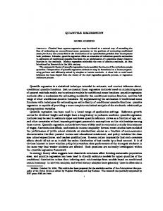
simulations where preformed in Stata 11 (StataCorp., 2009) using the command qreg2 (Machado, Parente, and Santos Silva, 2013) that implements both the covariance matrix estimator and the test studied here. Tables 1 and 2 give the rejection frequencies of the null hypothesis at the 5% level; we report the results obtained using both the covariance matrix estimator proposed in Section 2 and a covariance matrix estimator obtained using 100 cluster-bootstraps. In evaluating the results of these experiments we will follow Cochran (1952), who suggested that a test can be regarded as robust relative to a nominal level of 5% if its actual signi…cance level is between 4% and 6%. Given the number of replicas used in these experiments, we will consider that estimated rejection frequencies within the range 3:62% to 6:47% provide evidence consistent with the robustness of the test. In line with the …ndings for the case of independent observations reported by Buchinsky (1995), our results show that the bootstrap estimator performs well in most of the cases 9

^ 1A ^B ^ 1 , we see that there is some tendency to considered. As for the results based on B overreject the null when n = 100 and a slight tendency to under-reject for larger samples when the errors are heteroskedastic (h = 1) and there is no intra-cluster correlation (dv = 3 ^ 1A ^B ^ and d = 0). Crucially, the results obtained using B

1

are quite reasonable when they

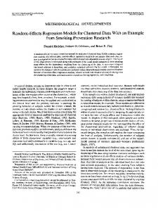
are more interesting, i.e., when the samples are large and the errors actually have intracluster correlation (dv = 2 and d = 1).8 ^ 1A ^B ^ Overall, the results obtained when using B

1

to estimate

are quite encouraging,

suggesting that this estimator can be used in situations where the bootstrap is impractical. Moreover, we note that although tests based on the bootstrap standard errors performed well in these experiments their use is not generally recommended (see, e.g., the comment in Davidson and MacKinnon, 2004, p. 208). Therefore, if bootstrap is at all feasible, it is perhaps better to use the processing time to obtain bootstrap con…dence intervals, or to

Table 1: Rejection frequencies at the 5% level (dv = 3 and d = 0) ^B ^ 1 ^ 1A B Bootstrap h n

G

0

100

0:0383

0:0675

0:1069

0:0508

0:0566

0:0585

1000

0:0541

0:0580

0:0641

0:0570

0:0571

0:0567

10000

0:0474

0:0515

0:0543

0:0515

0:0530

0:0578

100

0:0548

0:0716

0:0859

0:0576

0:0599

0:0580

1000

0:0511

0:0540

0:0517

0:0567

0:0576

0:0492

10000

0:0504

0:0522

0:0502

0:0527

0:0554

0:0500

100

0:0621

0:0684

0:1055

0:0567

0:0609

0:0624

1000

0:0340

0:0442

0:0551

0:0507

0:0590

0:0544

10000

0:0338

0:0374

0:0461

0:0512

0:0535

0:0564

100

0:0488

0:0546

0:0791

0:0574

0:0606

0:0603

1000

0:0356

0:0330

0:0457

0:0558

0:0479

0:0481

10000

0:0396

0:0370

0:0416

0:0561

0:0517

0:0493

2

5

1

2

5

8

= 0:25

= 0:50

= 0:75

= 0:25

= 0:50

= 0:75

We performed an additional set of experiments with a similar design but with normally distributed

^ errors and the results for the tests based on B

1^

^ AB

1

10

were slightly better than those reported here.

Table 2: Rejection frequencies at the 5% level (dv = 2 and d = 1) ^ 1A ^B ^ 1 B Bootstrap h n

G

0

100

0:0419

0:0677

0:1102

0:0545

0:0575

0:0604

1000

0:0482

0:0557

0:0612

0:0528

0:0585

0:0550

10000

0:0562

0:0554

0:0554

0:0615

0:0583

0:0566

100

0:0598

0:0740

0:0920

0:0632

0:0610

0:0644

1000

0:0520

0:0558

0:0616

0:0553

0:0567

0:0582

10000

0:0496

0:0487

0:0565

0:0520

0:0539

0:0601

100

0:0717

0:0721

0:1103

0:0660

0:0608

0:0667

1000

0:0332

0:0419

0:0582

0:0506

0:0539

00547

10000

0:0366

0:0398

0:0445

0:0543

0:0544

0:0510

100

0:0584

0:0630

0:0946

0:0627

0:0626

0:0663

1000

0:0375

0:0400

0:0566

0:0540

0:0514

0:0561

10000

0:0363

0:0364

0:0448

0:0481

0:0492

0:0501

2

5

1

2

5

= 0:25

= 0:50

= 0:75

= 0:25

= 0:50

= 0:75

^B ^ 1 . The study of the ^ 1A compute bootstrap p-values for the test statistics based on B performance of these methods is, however, beyond the scope of the present paper. The performance of the speci…cation test is again evaluated by computing the rejection frequencies at the 5% level of the null hypothesis, which in this case is de…ned by (6). The test is based on the statistic T =

XG

g=1

1 p G

Pn

i=1

Pn

j=1

(^ ugi )

q 2 2 (1

(^ ugi )2

(^ ugj )

, )2 n(n

1)

and in these experiments we took G 2 f100; 500; 1000g because the power of the test increases quickly with the sample size. Table 3 presents the rejection frequencies under the null (dv = 3 and d = 0) and Table 4 presents the results under the alternative (dv = 2 and d = 1). For comparison, the rejection frequencies obtained with the test suggested by Wooldridge (2002, p. 265) are also included in Tables 3 and 4.

11

Table 3: Rejection frequencies under the null (at 5%) = 0:25 h=0

h=1

= 0:50 h=0

h=1

= 0:75 h=0

h=1

Wooldridge

n

G

h=0

h=1

2

100 0:0494 0:0524 0:0566 0:0630 0:0496 0:0565 0:0513 0:0349 500 0:0493 0:0513 0:0501 0:0547 0:0539 0:0543 0:0512 0:0425 1000 0:0523 0:0483 0:0540 0:0516 0:0475 0:0456 0:0513 0:0449

5

100 0:0411 0:0401 0:0482 0:0498 0:0400 0:0399 0:0624 0:0506 500 0:0487 0:0470 0:0509 0:0510 0:0506 0:0510 0:0533 0:0557 1000 0:0522 0:0519 0:0570 0:0550 0:0513 0:0519 0:0540 0:0499

Table 4: Rejection frequencies under the alternative (at 5%) = 0:25 h=0

h=1

= 0:50 h=0

h=1

= 0:75 h=0

h=1

Wooldridge

n

G

h=0

h=1

2

100 0:4285 0:4385 0:6066 0:5998 0:6409 0:6427 0:7005 0:3343 500 0:9709 0:9685 0:9995 0:9998 0:9992 0:9991 0:9999 0:9096 1000 0:9997 0:9996 1:0000 1:0000 1:0000 1:0000 1:0000 0:9891

5

100 0:9962 0:9973 0:9998 0:9998 0:9963 0:9966 0:9493 0:7131 500 0:9999 1:0000 1:0000 1:0000 1:0000 1:0000 1:0000 0:9867 1000 1:0000 1:0000 1:0000 1:0000 1:0000 1:0000 1:0000 0:9974

Under the null all tests generally perform well and there is little to choose between them. Under the alternative the results depend on the value of h. In the heteroskedastic case (h = 1) the quantile-based tests clearly dominate Wooldridge’s test, whereas in the homoskedastic case (h = 1) the situation is reversed. However, for realistic sample sizes there is little to choose between the tests because their power quickly approaches 1.9 9

Notice, however, that the quantile-based tests have the advantage of not requiring that the errors have

…nite moments, and therefore are more generally valid than the test proposed by Wooldridge (2002).

12

5. CONCLUDING REMARKS We present the asymptotic results needed to perform inference with quantile regression when the data are obtained by sampling from di¤erent groups and it is assumed that observations from di¤erent groups are conditionally independent but intra-cluster correlation is not ruled out. We propose a consistent estimator of the covariance matrix of the asymptotic distribution of the estimator allowing for possible intra-cluster correlation and propose a simple test to check the presence of this type of correlation. The results of a small simulation study suggest that the proposed tools are likely to work reasonably well in practice.

APPENDIX Throughout the Appendix cr , CS, M, and T denote the cr , Cauchy-Schwarz, Markov, and triangle inequalities respectively. LLN denotes the Khintchine’s Weak Law of Large Numbers, UWL denotes a uniform weak law of large numbers such as Lemma 2.4 of Newey and McFadden (1994), and CLT is the Lindeberg-Lévy central limit theorem. Proof of Theorem 1: We use Theorem 2.7 of Newey and McFadden (1994). Note that ^ = arg minSG ( ) 2Rk

= arg min 2Rk

SG (

0)

1 XG Xn g=1 i=1 G

We have to show that SG ( )

SG (

0)

(ygi

x0gi )

1 XG Xn g=1 i=1 G

(ugi ) :

converges uniformly to a function. In this case

pointwise convergence su¢ ces as pointwise convergence of convex functions implies uniform convergence on compact subsets. Note that SG ( )

SG (

0)

1 XG Xn [ (ygi g=1 i=1 G 1 XG Xn [ (ugi = g=1 i=1 G

=

13

x0gi )

(ugi )]

x0gi )

(ugi )];

where

0.

Note that Knight’s identity (Koenker, 2005, p. 121) tells us that Z v (u v) (v) = v (u) + fI[u s] I[u 0]g ds;

=

0

where

I(u < 0). Thus

(u) = SG ( )

Now by a LLN to

SG (

1 G

0) =

PG Pn g=1

i=1

1 XG Xn x0gi (ugi ) i=1 g=1 G Z x0gi 1 XG Xn fI[ugi + i=1 0 g=1 G x0gi

S( ) =

s]

I[ugi

0]g ds:

(ugi ) = op (1) and the second term of the rhs converges

Xn

i=1

Z E[

x0gi

fF[sjxgi ]

0

g ds]:

Note that S( ) = 0 if and only if

= 0 and S( ) > 0 if 6= 0. To see this note that if R x0 > 0, thus 0 gi fF[sjxgi ] g ds > 0. If x0gi < 0 for some

x0gi > 0 for some i F[sjxgi ] R x0 i F[sjxgi ] < 0, thus 0 gi fF[sjxgi ]

g ds > 0. Since

minimizer and the limiting function is convex,

=

and the function is convex and consequently ^ =

0

=

0

0

= 0 is a unique local

= 0 is also a global minimizer

+ op (1).

Proof of Theorem 2: We adapt the proof of Koenker (2005, p. 121). Consider the objective function ZG ( ) =

XG Xn g=1

i=1

[ (ugi

This function is convex and minimized at ^G =

p x0gi = G) p

G( ^

0 ).

(ugi )]: Using Knight’s identity we

have ZG ( ) = Z1G ( ) + Z2G ( ) 1 XG Xn Z1G ( ) = p x0gi (ugi ) g=1 i=1 G XG Xn Z G 1=2 x0gi Z2G ( ) = fI[ugi s] g=1

i=1

0

14

I[ugi

0]g ds:

0

Now Z1G ( ) =

W , where W = G

1=2

PG Pn g=1

N (0; C) where

xgi

i=1

D

(ugi ). Also, by a CLT, W !

Xn C = Var( xgi (ugi )) i=1 Xn Xn = E[ xgi (ugi )( xgj (ugj ))0 ] i=1 j=1 Xn Xn xgi x0gj (ugi ) (ugj )]: = E[ j=1

i=1

Now write

Z

Z2Ggi ( ) = and Z2G ( ) =

PG Pn g=1

i=1

RG ( ) =

g=1

i=1

fI[ugi

s]

I[ugi

0]g ds;

Z2Ggi ( ). Note that

where

XG Xn

1=2 x0 gi

0

Z2G ( ) =

Note also that

G

XG Xn g=1

i=1

XG Xn g=1

i=1

E[Z2Ggi ( )jxgi ] + RG ( );

fZ2Ggi ( )

E[Z2Ggi ( )jxgi ]g :

XG Xn Z

E[Z2Gg ( )jxg ] =

g=1

i=1

G

1=2 x0 gi

fF[sjxgi ]

0

g ds

Z x0gi 1 XG Xn t p F[ 1=2 jxgi ] dt g=1 i=1 G G 0 Z x0gi t F[ G1=2 jxgi ] 1 XG Xn p tdt g=1 i=1 0 G t= G Z x0gi 1 XG Xn ff [0jxgi ]g tdt + op (1) g=1 i=1 0 G 1 XG Xn 0 f [0jxgi ]xgi x0gi + op (1): g=1 i=1 2G

= = = = Now by CS Z2Ggi ( ) =

Z

G

1=2 x0 gi

0

x0gi G1=2

fI[ugi k k kxgi k : G1=2 15

s]

I[ugi

0]g ds

(7)

Note that E[RG ( )] = 0 and that by cr , (7), and CS we have Var(RG ( )) =

XG

Xn E[( Z2Ggi ( ))2 ] g=1 i=1 XG Xn E[Z2Ggi ( )2 ] n g=1

i=1

k k XG Xn n 1=2 E[Z2Ggi ( ) kxgi k] i=1 g=1 G k k XG Xn E[E[Z2Ggi ( )jxgi ] kxgi k] = n 1=2 i=1 g=1 G Z x0gi t F[ G1=2 jxgi ] k k XG Xn p = n 3=2 E[kxgi k tdt] i=1 g=1 G t= G 0 k k XG Xn n 3=2 E[kxgi k 0 f [0jxgi ]xgi x0gi ] + o(1) g=1 i=1 2G k k3 X n E[kxgi k3 ] + o(1) n 1=2 f1 i=1 2G = o(1): Thus RG ( ) = op (1). Hence by a LLN 1 XG Xn 0 f [0jxgi ]xgi x0gi + op (1) g=1 i=1 2G = 0 B =2 + op (1):

Z2G ( ) =

Therefore ZG ( ) = The convexity of p

G( ^

0

0

W + 0 B =2 + op (1):

W + 0 B =2 assures that the minimizer is unique and therefore 0)

D

= arg min ZG ( ) ! ^0 = arg min

0

W + 0 B =2:

Now note that ^0 = B 1 W (see Koenker, 2005, p. 122, and the references therein). Proof of Theorem 3: The proof is similar to that of Lemma 5 of Kim and White (2003). P Pn Let BG = (2cG G) 1 G cG )xgi x0gi . Using the mean value theorem we have g=1 i=1 I(jugi j P E[BG ] = E[ ni=1 f (~ cG jxgi )xgi x0gi ], where j~ cG j cG and therefore c~G = o(1). Hence, by the Lebesgue dominated convergence theorem E[BG ] = B. It follows from the law of large num-

bers for double arrays (Davidson, 1994, Corollary 19.9, p. 301, and Theorem 12.10, p. 190) 16

p ~G that BG ! B. We now show (i) B

p ~ G = (2cG G) BG ! 0 where B

~G To prove (i) consider the (h; j)th element of B (2cG G)

1

XG Xn

i=1

g=1

[I(j^ ugi j

0)

I(y

0)j

jx

I(jxj

I(j^ ugi j

cG )]xgih x0gij :

I(jugi j

0 0 ) xgi ,

yj), jI(x < 0)

i=1

BG , which is given by

c^G )

(^

Now using the facts that u^gi = ugi

PG Pn g=1

p ~G ! B 0. The conclusion follows from T.

^ c^G )xgi x0gi , and (ii) B

jI(x

1

I(jaj

b) = I(a

I(y < 0)j

I(jxj

b) jx

I(a
g, D2G > 0. Thus

i=1

I(jugi j

U1G + U2G

cG )]xgih xgij cG j

dG )] jxgih j jxgij j

[I(jugi + cG j

dG )] jxgih j jxgij j ;

g=1 i=1 XG Xn g=1

c^G j + ^

similar.

a constant

1

[I(j^ ugi j c^G ) XG Xn

[I(jugi

p

p

kxgi k. We prove that U1G ! 0, the proof U2G ! 0 is

n = cG1 ^

o , and D3G = cG1 jcG

0

c^G j

for

Pr(U1G > ) = Pr(D1G ) c c Pr(D1G \ D2G \ D3G ) + Pr(D2G ) + Pr(D3G ):

Now as

p

G( ^

0)

p c = Op (1) and cG1 = o( G) it follows that limG!1 Pr(D2G ) = 0.

p c Also as c^G =cG ! 1, we have limG!1 Pr(D3G ) = 0. Additionally if cG1 ^

cG1 jcG

c^G j

we have jdG j

Pr(D1G \ D2G \ D3G )

cG

(2 cG G) (2 cG G) = ( )

1

under Assumptions 3. Now take

+ cG 1

XG

g=1

1

g=1

i=1

and

kxgi k. Hence by M Z cG +cG kxgi k Xn E[ f (sjxgi )ds jxgih j jxgij j] i=1

XG Xn

Xn

0

i=1

Z E[

cG

cG kxgi k

cG +cG kxgi k cG

cG kxgi k

f1 ds jxgih j jxgij j]

E[(kxgi k + 1) jxgih j jxgij j] < 1 p

arbitrarily small and consequently U1G ! 0. 17

^ To prove (ii), note that B since

cG c^G

~G = B

~ G . Note also that by (i) B ~ G = Op (1) and 1 B

cG c^G

1 = op (1) by assumption, the result follows.

Proof of Theorem 4: For simplicity of notation we write P Pn j := j=1 . Note that T

where

P

gi

:=

PG Pn g=1

1 X X 2 = p zgi zgj (^ ugi ) (^ ugj ) (^ ugi )2 zgi gi j G 1 X X zgi zgj (^ ugi ) (^ ugj ) = p gi j;i6=j G 1 X X = p zgi zgj (ugi ) (ugj ) + RG ; gi j;i6=j G

1 X X zgi zgj [ RG = p gi j;i6=j G Now by Lemma 5 RG =

where hgij ( ^ ) =

(^ ugj )

(ugi )

(ugj )] :

1 X X zgi zgj hgij ( ^ ) + op (1); gi j;i6=j G1=2 F(x0gj ( ^

2

+F(x0gi ( ^ By a Taylor expansion around RG =

(^ ugi )

0

0 )jxgj )

0 )jxgi )

F(x0gi ( ^

F(x0gj ( ^

0 )jxgj ),

i 6= j:

we have

p 1 X X zgi zgj Hgij ( ~ ) G( ^ gi j; i6=j G

where ~ is on the line segment joining ^ and f (x0gj ( ~

Hgij ( ~ ) =

0 )jxgi )

0

+f (x0gi ( ~

0 )jxgi )

+f (x0gj ( ~

0 ~ 0 )jxgj )F(xgi (

f (x0gi ( ~

F(x0gj ( ~

0 0 )jxgi )xgi

0 0 )jxgj )xgi 0 0 )jxgi )xgj ;

1 X X zgi zgj Hgij ( ~ ) = op (1) gi j;i6=j G 18

+ op (1);

and

0 0 )jxgj )xgj

where i 6= j. Now notice that

0)

i=1

and

by a UWL. Since

p G( ^

= Op (1) we have RG = op (1). Thus 1 X X T =p zgi zgj (ugi ) (ugj ) + op (1) gi j;i6=j G 0)

and consequently T ! N (0; D) as D > 0 and i 2 Xn hXn zgi zgj (ugi ) (ugj ) ] D = E[ j=1;i6=j i=1 Xn Xn 4 1=2 2 4 1=2 ] ( + 1)2 < 1 ] E[zgj n E[zgi i=1

j=1;i6=j

by two applications of cr and one of CS. Let mG ( ) =

1 X X zgi zgj [ gi j;i6=j G

x0ig (

I(ugi

0 ))][

I(ugj

x0gi (

0 ))]

:

Lemma 5 Suppose that Assumption 4 holds. Then, under H0 , for any G = o(1) we have p 1 X X sup G(mG ( ) mG ( 0 )) zgi zgj hgij ( ) = op (1); gi j;i6=j G1=2 k G 0k

where

2

hgij ( ) =

F(x0gj (

+F(x0gi ( Proof: Note that mG ( ) = where hgij ( ) = [ +I(ugi

2

F(x0gj (

0 )jxgi )

0 )jxgi ) 0 )jxgj ):

1 X X zgi zgj hgij ( ); gi j;i6=j G

I(ugj

x0ig (

F(x0gi (

0 )jxgj )

x0gj (

0 ))

I(ugi

x0gj (

0 ))I(ugj

0 ))],

x0gi (

0 ))

i 6= j:

Now taking the expected value of hgij ( ) conditional on xg we have E[hgij ( )jxg ] =

2

Fj (x0gj (

0 )jxg )

+Fi;j (x0ig ( =

2

0 0 ); xgj (

F(x0gj (

+F(x0gi (

19

0 )jxg )

0 )jxg )

0 )jxgj ) 0 )jxgi )

+ Fi (x0gi (

+ F(x0gi (

F(x0gj (

0 )jxgi ) 0 )jxgj );

where the last line follows from H0 and i 6= j. Note now that p

G(mG ( ) mG ( 1 X X G1=2

gi

0 ))

j;i6=j

1 X X zgi zgj hgij ( ) = gi j;i6=j G1=2

zgi zgj [hgij ( )

Since the indicator functions I(ugi ditional distribution functions F(x0gi (

x0ig (

hgij (

0 )) 0 )jxgi )

0)

and I(ugj

and F(x0gj (

hgij ( )]. x0gi (

0 )jxgj )

0 ))

and the con-

are functions of

bounded variation (and hence type I class of functions in the sense of Andrews, 1994) and as Assumptions 1 (a) and 4 (a) hold, it follows that 1 X X zgi zgj [hgij ( ) gi j;i6=j G1=2

hgij (

0)

hgij ( )]

is stochastic equicontinuous by Theorems 1, 2 and 3 of Andrews (1994).

20

REFERENCES Abrevaya, J. and Dahl, C.M. (2008). “The E¤ects of Birth Inputs on Birthweight,” Journal of Business & Economic Statistics, 26, 379-397. Andrews, D.W.K. (1994). “Empirical Process Methods in Econometrics,” in R.F. Engle and D.L. McFadden, eds., Handbook of Econometrics, Vol. 4, 2247-2294. New York(NY): North Holland. Arellano, M. (1987). “Computing Robust Standard Errors for Within-Group Estimators,” Oxford Bulletin of Economics and Statistics, 49, 431-434. Bhattacharya, D. (2005). “Asymptotic Inference from Multi-Stage Samples,” Journal of Econometrics, 126, 145-171. Breusch, T.S. and Pagan, A.R. (1980). “The Lagrange Multiplier Test and its Applications to Model Speci…cation in Econometrics,”Review of Economic Studies, 47, 239-253. Buchinsky, M. (1995), “Estimating the Asymptotic Covariance Matrix for Quantile Regression Models a Monte Carlo Study,”Journal of Econometrics, 68, 303-38. Cameron, A.C. and Miller, D.L. (2011). “Robust Inference with Clustered Data,” in A. Ullah and D.E. Giles, eds., Handbook of Empirical Economics and Finance, 1-28, Boca Raton (FL): Chapman & Hall/CRC Press. Chamberlain, G. (1994). “Quantile Regression, Censoring and the Structure of Wages,” in C.A. Sims, ed., Advances in Econometrics, 171–209. Cambridge: Cambridge University Press. Cochran, W.G. (1952). “The

2

Test of Goodness of Fit,” Annals of Mathematical Sta-

tistics, 23, 315-345. Davidson, J.E.H. (1994). Stochastic Limit Theory. Oxford: Oxford University Press. Davidson, R. and MacKinnon, J.G. (2004). Econometric Theory and Methods. New York, Oxford University Press.

21

Fitzenberger, B., Kohn, K. and Lembcke, A.C. (2013). “Union Density and Varieties of Coverage: The Anatomy of Union Wage E¤ects in Germany,” Industrial & Labor Relations Review, 66, 169-197. Kim, T.H. and White, H. (2003). “Estimation, Inference, and Speci…cation Testing for Possibly Misspeci…ed Quantile Regressions,” in T. Fomby and R.C. Hill, eds., Maximum Likelihood Estimation of Misspeci…ed Models: Twenty Years Later, 107-132. New York (NY): Elsevier. Koenker, R. (2005). Quantile Regression. New York (NY): Cambridge University Press. Koenker, R. and Bassett, G. (1978). “Regression Quantiles,”Econometrica, 46, 33-50. Koenker, R. and Machado, J.A.F. (1999).

“Goodness of Fit and Related Inference

Processes for Quantile Regression”, Journal of the American Statistical Association, 94, 1296-1310. Liang, K.-Y. and Zeger, S.L. (1986). “Longitudinal Data Analysis Using Generalized Linear Models,”Biometrika, 73, 13-22. Machado, J.A.F., Parente, P.M.D.C, and Santos Silva, J.M.C. (2013). qreg2: Stata module to perform quantile regression with robust and clustered standard errors, Statistical Software Components S457369, Boston College Department of Economics. Moulton, B.R. (1986), “Random Group E¤ects and the Precision of Regression Estimates,”Journal of Econometrics, 32, 385-97. Moulton, B.R. (1990), “An Illustration of a Pitfall in Estimating the E¤ects of Aggregate Variables on Micro Units,”Review of Economics and Statistics, 72, 334-38. Newey, W.K. and McFadden, D.L. (1994). “Large Sample Estimation and Hypothesis Testing”, in R.F. Engle and D.L. McFadden, eds., Handbook of Econometrics, Vol. 4, 2111-2245. New York (NY): North Holland. Penner, A.M. (2008). “Gender Di¤erences in Extreme Mathematical Achievement: An International Perspective on Biological and Social Factors,” American Journal of Sociology, 114, S138-S170. 22

Powell, J.L. (1984).

“Least Absolute Deviation Estimation for Censored Regression

Model”, Journal of Econometrics, 25, 303-325. Powell, J.L. (1986). “Censored Regression Quantiles”, Journal of Econometrics, 32, 143155. Rogers, W.H. (1993), “Regression Standard Errors in Clustered Samples,”Stata Technical Bulletin, 13, 19-23. StataCorp. (2009). Stata Release 11. Statistical Software. College Station (TX): StataCorp LP. White, H. (1980), “A Heteroskedasticity-Consistent Covariance Matrix Estimator and a Direct Test for Heteroskedasticity,”Econometrica, 48, 817–838. White, H. (1984), Asymptotic Theory for Econometricians, San Diego (CA): Academic Press. Wooldridge, J.M. (2002). Econometric Analysis of Cross Section and Panel Data, Cambridge(MA): MIT Press.

23