inference has been forged from the theory of the dual regression quantile process, ... Just as classical linear regression methods based on minimizing sums ... regression is capable of providing a more complete statistical analysis of the ... used to estimate upper and lower quantile reference curves as a function of age, sex,.
QUANTILE REGRESSION ROGER KOENKER
Abstract. Classical least squares regression may be viewed as a natural way of extending the
idea of estimating an unconditional mean parameter to the problem of estimating conditional mean functions; the crucial link is the formulation of an optimization problem that encompasses both problems. Likewise, quantile regression o�ers an extension of univariate quantile estimation to estimation of conditional quantile functions via an optimization of a piecewise linear objective function in the residuals. Median regression minimizes the sum of absolute residuals, an idea introduced by Boscovich in the 18th century. The asymptotictheory of quantile regressionclosely parallelsthe theory of the univariatesample quantiles. Computation of quantile regression estimators may be formulated as a linear programming problem and e�ciently solved by simplex or barrier methods. A close link to rank based inference has been forged from the theory of the dual regression quantile process, or regression rankscore process.
Quantile regression is a statistical technique intended to estimate, and conduct inference about, conditional quantile functions. Just as classical linear regression methods based on minimizing sums of squared residuals enable one to estimate models for conditional mean functions, quantile regression methods o�er a mechanism for estimating models for the conditional median function, and the full range of other conditional quantile functions. By supplementing the estimation of conditional mean functions with techniques for estimating an entire family of conditional quantile functions, quantile regression is capable of providing a more complete statistical analysis of the stochastic relationships among random variables. Quantile regression has been used in a broad range of application settings. Reference growth curves for childrens' height and weight have a long history in pediatric medicine; quantile regression methods may be used to estimate upper and lower quantile reference curves as a function of age, sex, and other covariates without imposing stringent parametric assumptions on the relationships among these curves. Quantile regression methods have been widely used in economics to study determinents of wages, discrimination e�ects, and trends in income inequality. Several recent studies have modeled the performance of public school students on standardized exams as a function of socio-economic characteristics like their parents' income and educational attainment, and policy variables like class size, school expenditures, and teacher quali cations. It seems rather implausible that such covariate e�ects should all act so as to shift the entire distribution of test results by a xed amount. It is of obvious interest to know whether policy interventions alter performance of the strongest students in the same way that weaker students are a�ected. Such questions are naturally investigated within the quantile regression framework. In ecology, theory often suggests how observable covariates a�ect limiting sustainable population sizes, and quantile regression has been used to directly estimate models for upper quantiles of the conditional distribution rather than inferring such relationships from models based on conditional central tendency. In survival analysis, and event history analysis more generally, there is often also a Version: October 25, 2000. This article has been prepared for the statistics section of the International Encycloedited by Stephen Fienberg and Jay Kadane. The research was partially supported by NSF grant SBR-9617206. 1
pedia of the Social Sciences
2
ROGER KOENKER
desire to focus attention on particular segments of the conditional distribution, for example survival prospects of the oldest-old, without the imposition of global distributional assumptions. 1. Quantiles, Ranks and Optimization We say that a student scores at the �th quantile of a standardized exam if he performs better than the proportion �, and worse than the proportion (1 , �), of the reference group of students. Thus, half of the students perform better than the median student, and half perform worse. Similarly, the quartiles divide the population into four segments with equal proportions of the population in each segment. The quintiles divide the population into 5 equal segments; the deciles into 10 equal parts. The quantile, or percentile, refers to the general case. More formally, any real valued random variable, Y , may be characterized by its distribution function, F (y) = Prob(Y � y) while for any 0 < � < 1, Q(�) = inf fy : F(y) � � g is called the �th quantile of X. The median, Q(1=2), plays the central role. Like the distribution function, the quantile function provides a complete characterization of the random variable, Y. The quantiles may be formulated as the solution to a simple optimization problem. For any 0 < � < 1, de ne the piecewise linear \check function", �� (u) = u(� , I(u < 0)) illustrated in Figure 1. ρτ (u)
τ−1
τ
Figure 1. Quantile Regression � Function
Minimizing the expectation of �� (Y , �) with respect to � yields solutions, �^(�), the smallest of which is Q(�) de ned above. The sample analogue of Q(�), based on a random sample, fy1; :::; yng, of Y 's, is called the �th sample quantile, and may be found by solving, min �2R
Xn � (y , �); i=1
� i
QUANTILE REGRESSION
3
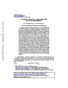
While it is more common to de ne the sample quantiles in terms of the order statistics, y(1) � y(2) � ::: � y(n) , constituting a sorted rearrangement of the original sample, their formulation as a minimization problem has the advantage that it yields a natural generalization of the quantiles to the regression context. Just as the idea of estimating the unconditional mean, viewed as the minimizer, X �^ = argmin�2jR (yi , �)2 can be extended to estimation of the linear conditional mean function E(Y jX = x) = x0 by solving, X ^ = argmin 2jRp (yi , x0i )2 ; the linear conditional quantile function, QY (� jX = x) = x0i (�), can be estimated by solving, X ^(�) = argmin 2jRp �� (yi , x0 ): The median case, � = 1=2, which is equivalent to minimizing the sum of absolute values of the residuals has a long history. In the mid-18th century Boscovich proposed estimating a bivariate linear model for the ellipticity of the earth by minimizing the sum of absolute values of residuals subject to the condition that the mean residual took the value zero. Subsequent work by Laplace characterized Boscovich's estimate of the slope parameter as a weighted median and derived its asymptotic distribution. F.Y. Edgeworth seems to have been the rst to suggest a general formulation of median regression involving a multivariate vector of explanatory variables, a technique he called the \plural median". The extension to quantiles other than the median was introduced in Koenker and Bassett (1978). 2. An Example To illustrate the approach we may consider an analysis of a simple rst order autoregressive model for maximum daily temperature in Melbourne, Australia. The data are taken from Hyndman, Bashtannyk, and Grunwald (1996). In Figure 2 we provide a scatter plot of 10 years of daily temperature data: today's maximum daily temperature is plotted against yesterday's maximum. Our rst observation from the plot is that there is a strong tendency for data to cluster along the (dashed) 45 degree line implying that with high probability today's maximum is near yesterday's maximum. But closer examination of the plot reveals that this impression is based primarily on the left side of the plot where the central tendency of the scatter follows the 45 degree line very closely. On the right side, however, corresponding to summer conditions, the pattern is more complicated. There, it appears that either there is another hot day, falling again along the 45 degree line, or there is a dramatic cooling o�. But a mild cooling o� appears to be more rare. In the language of conditional densities, if today is hot, tomorrow's temperature appears to be bimodal with one mode roughly centered at today's maximum, and the other mode centered at about 20�. Several estimated quantile regression curves have been superimposed on the scatterplot. Each curve is speci ed as a linear B-spline. Under winter conditions these curves are bunched around the 45 degree line, however in the summer it appears that the upper quantile curves are bunched around the 45 degree line and around 20� . In the intermediate temperatures the spacing of the quantile curves is somewhat greater indicating lower probability of this temperature range. This impression is strengthened by considering a sequence of density plots based on the quantile regression estimates. Given a family of reasonably densely spaced estimated conditional quantile functions, it is straightforward to estimate the conditional density of the response at various values of the conditioning covariate. In Figure 3 we illustrate this approach with several of density estimates based on the Melbourne data. Conditioning on a low previous day temperature we see a nice
4
ROGER KOENKER
. . .. . . .. . .... .. .. .. ... .. . . . .. . . . . . . . .. . . ... . . . . .... .. .. ...... ... . .... .. . . .. .... .. . ... .... . ... .. .......... . . . . . .. . . . . .. . ..... ....... .. ........ .. ... ...... .................... .... . . . .. . . . . . . . . .. . . ... . .. ... . . .. . . . ............................ .... ......... .. ... ... ..... . . .... . . . .. ..................... ............... ...... .... . .. . . .. . . . . . . . . . .. . . ................................................................. .. .......... . ...... .... .. .. . . . . ...... .. .................................................... ... . .. .. .. .. . . . . . .... . .... .. . .... .. .. .. .. . . .. . ... .... ............................................................... ...... ..................... .... .... ..... . .. ... ... . .... ............................................................................................................... . ............. . ...... . ........ ............................................................................................ ... ....... .. . . .. ... .... . . ... .. ............................................................... ....................... .... . ... . .. ... . ................................................... . . . . .. .. . . . . ... . . . .... ............................................................................................ ............. .... .. .. ..... . ..... . . . . . ... ................................ ........... .... ... ... . . . . . ....................................... . .......................................... ...... ... . .... . . . . . . . . ................................................................................. .. .. . . . . . . . .. . . ................................................................................ ......... .... .. . . . . . . . . . . . . . . . .. ....... ...... . .. ...................... . . . . . ... .
30 20 10
today’s max temperature
40
.
10
15
20
25
30
35
40
yesterday’s max temperature Figure 2. Melbourne Maximum Daily Temperature: The plot illustrates 10 years
of daily maximum temperature data (in degrees centigrade) for Melbourne, Australia as an AR(1) scatterplot. The data is scattered around the (dashed) 45 degree line suggesting that today is roughly similar to yesterday. Superimposed on the scatterplot are estimated conditional quantile functions for the quantiles � 2 f:05; :10; :::;:95g. Note that when yesterday's temperature is high the spacing between adjacent quantile curves is narrower around the 45 degree line and at about 20 degrees Centigrade than it is in the intermediate region. This suggests bimodality of the conditional density in the summer.
QUANTILE REGRESSION Yesterday’s Temp 16
Yesterday’s Temp 21
12
14
16
0.10 0.02
0.06
density
0.10
density
0.02 10
12
14
16
18
20 22
24
15
20
25
30
today’s max temperature
today’s max temperature
Yesterday’s Temp 25
Yesterday’s Temp 30
Yesterday’s Temp 35
20
25
30
35
today’s max temperature
0.05 0.01
0.01 15
0.03
density
density
0.03
0.03
0.05
0.05
today’s max temperature
0.01
density
0.06
0.10 0.05
density
0.15
0.14
Yesterday’s Temp 11
5
20
25
30
35
today’s max temperature
40
20
25
30
35
40
today’s max temperature
Figure 3. Conditional density estimates of today's maximum temperature for sev-
eral values of yesterday's maximum temperature based on the Melbourne data: These density estimates are based on a kernel smoothing of the conditional quantile estimates as illustrated in the previous gure using 99 distinct quantiles. Note that temperature is bimodal when yesterday was hot.
unimodal conditional density for the following day's maximum temperature, but as the previous day's temperature increases we see a tendency for the lower tail to lengthen and eventually we see a clearly bimodal density. In this example, the classical regression assumption that the covariates a�ect only the location of the response distribution, but not its scale or shape, is violated. 3. Interpretation of Quantile Regression Least squares estimation of mean regression models asks the question, \How does the conditional mean of Y depend on the covariates X?" Quantile regression asks this question at each quantile of the conditional distribution enabling one to obtain a more complete description of how the conditional distribution of Y given X = x depends on x. Rather than assuming that covariates shift only the location or scale of the conditional distribution, quantile regression methods enable one to explore potential e�ects on the shape of the distribution as well. Thus, for example, the e�ect of a jobtraining program on the length of participants' current unemployment spell might be to lengthen the shortest spells while dramatically reducing the probability of very long spells. The mean treatment
6
ROGER KOENKER
e�ect in such circumstances might be small, but the treatment e�ect on the shape of the distribution of unemployment durations could, nevertheless, be quite signi cant. 3.1. Quantile Treatment E�ects. The simplest formulation of quantile regression is the twosample treatment-control model. In place of the classical Fisherian experimental design model in which the treatment induces a simple location shift of the response distribution, Lehmann (1974) proposed the following general model of treatment response: \Suppose the treatment adds the amount �(x) when the response of the untreated subject would be x. Then the distribution G of the treatment responses is that of the random variable X + �(X) where X is distributed according to F." Special cases obviously include the location shift model, �(X) = �0, and the scale shift model, �(X) = �0X, but the general case is natural within the quantile regression paradigm. Doksum (1974) shows that if �(x) is de ned as the \horizontal distance" between F and G at x, so F(x) = G(x + �(x)) then �(x) is uniquely de ned and can be expressed as �(x) = G,1(F (x)) , x: Changing variables so � = F(x) one may de ne the quantile treatment e�ect, �(�) = �(F ,1(�)) = G,1(�) , F ,1(�): In the two sample setting this quantity is naturally estimable by �^(�) = G^ ,n 1(�) , F^m,1(�) where Gn and Fm denote the empirical distribution functions of the treatment and control observations, based on n and m observations respectively. Formulating the quantile regression model for the binary treatment problem as, QYi (� jDi) = �(�) + �(�)Di where Di denotes the treatment indicator, with Di = 1 indicating treatment, Di = 0, control, then the quantile treatment e�ect can be estimated by solving, Xn (^�(�); �^(�))0 = argmin �� (yi , � , �Di ): i=1
The solution (^�(�); �^(�))0 yields �^ (�) = F^n,1(�), corresponding to the control sample, and �^(�) = G^ ,n 1(�) , F^n,1(�): Doksum suggests that one may interpret control subjects in terms of a latent characteristic: for example in survival analysis applications, a control subject may be called frail if he is prone to die at an early age, and robust if he is prone to die at an advanced age. This latent characteristic is thus implicitly indexed by �, the quantile of the survival distribution at which the subject would appear if untreated, i.e., (Yi jDi = 0) = �(�): And the treatment, under the Lehmann model, is assumed to alter the subjects control response, �(�), making it �(�) + �(�) under the treatment. If the latent characteristic, say, the propensity for longevity, were observable ex ante, then one could view the treatment e�ect �(�) as an explicit interaction with this observable variable. In the absence of such
QUANTILE REGRESSION
7
an observable variable however, the quantile treatment e�ect may be regarded as a natural measure of the treatment response. It may be noted that the quantile treatment e�ect is intimately tied to the two-sample QQ-plot ^ = G,n 1(Fm (x)) , x is which has a long history as a graphical diagnostic device. The function �(x) exactly what is plotted in the traditional two sample QQ-plot. If F and G are identical then the function G,n 1(Fm (x)) will lie along the 45 degree line; if they di�er only by a location scale shift, then G,n 1 (Fm (x)) will lie along another line with intercept and slope determined by the location and scale shift, respectively. Quantile regression may be seen as a means of extending the two-sample QQ plot and related methods to general regression settings with continuous covariates. When the treatment variable takes more than two values, the Lehmann-Doksum quantile treatment e�ect requires only minor reinterpretation. If the treatment variable is continuous as, for example, in dose-response studies, then it is natural to consider the assumption that its e�ect is linear, and write, QYi (� jxi) = �(�) + (�)xi : We assume thereby that the treatment e�ect, (�), of changing x from x0 to x0 +1 is the same as the treatment e�ect of an alteration of x from x1 to x1 +1: Note that this notion of the quantile treatment e�ect measures, for each �, the change in the response required to stay on the �th conditional quantile function. 3.2. Transformation Equivariance of Quantile Regression. An important property of the quantile regression model is that, for any monotone function, h(�), Qh(T ) (� jx) = h(QT (� jx)): This follows immediately from observing that Prob(T < tjx) = Prob(h(T) < h(t)jx): This equivariance to monotone transformations of the conditional quantile function is a crucial feature, allowing one to decouple the potentially con icting objectives of transformations of the response variable. This equivariance property is in direct contrast to the inherent con icts in estimating transformation models for conditional mean relationships. Since, in general, E(h(T )jx) 6= h(E(T jx)) the transformation alters in a fundamental way what is being estimated in ordinary least squares regression. A particularly important application of this equivariance result, and one that has proven extremely in uential in the econometric application of quantile regression, involves censoring of the observed response variable. The simplest model of censoring may be formulated as follows. Let yi� denote a latent (unobservable) response assumed to be generated from the linear model yi� = x0i + ui i = 1; : : : ; n with fuig iid from distribution function F. Due to censoring, the yi� 's are not observed directly, but instead one observe yi = maxf0; yi� g: Powell (1986) noted that the equivariance of the quantiles to monotone transformations implied that in this model the conditional quantile functions of the response depended only on the censoring point, but were independent of F. Formally, the �th conditional quantile function of the observed response, yi ; in this model may be expressed as Qi (� jxi) = maxf0; x0i + Fu,1(�)g
8
ROGER KOENKER
The parameters of the conditional quantile functions may now be estimated by solving min b
Xn � (y , maxf0; x0bg) i=1
� i
i
where it is assumed that the design vectors xi, contain an intercept to absorb the additive e�ect of Fu,1(�): This model is computationally somewhat more demanding than conventional linear quantile regression because it is non-linear in parameters. 3.3. Robustness. Robustness to distributional assumptions is an important consideration throughout statistics, so it is important to emphasize that quantile regression inherits certain robustness properties of the ordinary sample quantiles. The estimates and the associated inference apparatus have an inherent distribution-free character since quantile estimation is in uenced only by the local behavior of the conditional distribution of the response near the speci ed quantile. Given a solution ^(�), based on observations, fy; X g, as long as one doesn't alter the sign of the residuals, any of the y observations may be arbitrary altered without altering the initial solution. Only the signs of the residuals matter in determining the quantile regression estimates, and thus outlying responses in uence the t in so far as they are either above or below the tted hyperplane, but how far above or below is irrelevant. While quantile regression estimates are inherently robust to contamination of the response observations, they can be quite sensitive to contamination of the design observations, fxig. Several proposals have been made to ameliorate this e�ect. 4. Computational Aspects of Quantile Regression Although it was recognized by a number of early authors, including Gauss, that solutions to the median regression problem were characterized by an exact t through p sample observations when p linear parameters are estimated, no e�ective algorithm arose until the development of linear programming in the 1940's. It was then quickly recognized that the median regression problem could be formulated as a linear program, and the simplex method employed to solve it. The algorithm of Barrodale and Roberts (1973) provided the rst e�cient implementation speci cally designed for median regression and is still widely used in statistical software. It can be concisely described as follows. At each step, we have a trial set of p \basic observations" whose exact t may constitute a solution. We compute the directional derivative of the objective function in each of the 2p directions that correspond to removing one of the current basic observations, and taking either a positive or negative step. If none of these directional derivatives are negative the solution has been found, otherwise one chooses the most negative, the direction of steapest descent, and goes in that direction until the objective function ceases to decrease. This one dimensional search can be formulated as a problem of nding the solution to a scalar weighted quantile problem. Having chosen the step length, we have in e�ect determined a new observation to enter the basic set, a simplex pivot occurs to update the current solution, and the iteration continues. This modi ed simplex strategy is highly e�ective on problems with a modest number of observations, achieving speeds comparable to the corresponding least squares solutions. But for larger problems with, say n > 100; 000 observations, the simplex approach eventually becomes considerably slower than least squares. For large problems recent development of interior point methods for linear programming problems are highly e�ective. Portnoy and Koenker (1997) describe an approach that combines some statistical preprocessing with interior point methods and achieves comparable performance to least squares solutions even in very large problems.
QUANTILE REGRESSION
9
An important feature of the linear programming formulation of quantile regression is that the entire range of solutions for � 2 (0; 1) can be e�ciently computed by parametric programming. At any solution ^(�0 ) there is an interval of �'s over which this solution remains optimal, it is straightforward to compute the endpoints of this interval, and thus one can solve iteratively for the entire sample path ^(�) by making one simplex pivot at each of the endpoints of these intervals. 5. Statistical Inference for Quantile Regression The asymptotic behavior of the quantile regression process f ^(�) : � 2 (0; 1)g closely parallels the theory of ordinary sample quantiles in the one sample problem. Koenker and Bassett (1978) show that in the classical linear model, yi = xi + ui withp ui iid from dfF; with density f(u) > 0 on its support fuj0 < F (u) < 1g, the joint distribution of n( ^n (�i ) , (�i ))mi,1 is asymptotically normal with mean 0 and covariance matrix D,1 . P Here (�) = + Fu,1(�)e1 ; e1 = (1; 0; : : : ; 0)0; x1i � 1; n,1 xi x0i ! D; a positive de nite matrix, and
= (!ij = (minf�i ; �j g , �i�j )=(f(F ,1 (�i ))f(F ,1 (�j ))): When the response is conditionally independent over i, but not identically distributed, the as^ , (�)) is somewhat more complicated. Let ymptotic covariance matrix of �(�) = pn( (�) �i (�) = xi (�) denote the conditional quantile function of y given xi , and fi (�) the corresponding conditional density, and de ne, Jn (�1; �2 ) = (minf�1 ; �2g , �1�2 )n,1 and
X
Xn x x0 ; i=1
i i
Hn(�) = n,1 xi x0i fi (�i (�)): Under mild regularity conditions on the ffi g's and fxi g's, we have joint asymptotic normality for vectors (�(�i ); : : : ; �(�m )) with mean zero and covariance matrix Vn = (Hn(�i ),1 Jn(�i ; �j )Hn (�j ),1)mi=1 : An important link to the classical theory of rank tests was made by Gutenbrunner and Jure�ckov�a (1992), who showed that the rankscore functions of H�ajek and S�id�ak (1967) could be viewed as a special case of a more general formulation for the linear quantile regression model. The formal dual of the quantile regression linear programming problem may be expressed as, maxfy0 ajX 0 a = (1 , t)X 0 1; a 2 [0; 1]ng: The dual solution a^(�) reduces to the H�ajek and S�id�ak rankscores process when the design matrix, X, takes the simple form of an n vector of ones. The regression rankscore process ^a(�) behaves asymptotically much like the classical univariate rankscore process, and thus o�ers a way to extend many rank based inference procedures to the more general regression context.
10
ROGER KOENKER
6. Extensions and Future Developments There is considerable scope for further development of quantile regression methods. Applications to survival analysis and time-series modeling seem particularly attractive, where censoring and recursive estimation pose, respectively, interesting challenges. For the classical latent variable form of the binary response model where, yi = I(x0i + ui � 0) and the median of ui conditional on xi is assumed to be zero for all i = 1; :::; n, Manski (1975) proposed an estimator solving, X(y , 1=2)I(x0 b � 0): max i i jjbjj=1 This \maximum score" estimator can be viewed as a median version of the general linear quantile regression estimator for binary response, X � (y , I(x0 b � 0)): min � i i jjbjj=1 In this formulation it is possible to estimate a family of quantile regression models and explore, semi-parametrically, a full range of linear conditional quantile functions for the latent variable form of the binary response model. Koenker and Machado (1999) introduce inference methods closely related to classical goodness of t statistics based on the full quantile regression process. There have been several proposals dealing with generalizations of quantile regression to nonparametric response functions involving both local polynomial methods and splines. Extension of quantile regression methods to multivariate response models is a particularly important challenge. 7. Conclusion Classical least squares regression may be viewed as a natural way of extending the idea of estimating an unconditional mean parameter to the problem of estimating conditional mean functions; the crucial step is the formulation of an optimization problem that encompasses both problems. Likewise, quantile regression o�ers an extension of univariate quantile estimation to estimation of conditional quantile functions via an optimization of a piecewise linear objective function in the residuals. Median regression minimizes the sum of absolute residuals, an idea introduced by Boscovich in the 18th century. The asymptotic theory of quantile regression closely parallels the theory of the univariate sample quantiles; computation of quantile regression estimators may be formulated as a linear programming problem and e�ciently solved by simplex or barrier methods. A close link to rank based inference has been forged from the theory of the dual regression quantile process, or regression rankscore process. Recent non-technical introductions to quantile regression are provided by Buchinsky (1998) and Koenker (2001). A more complete introduction will be provided in the forthcoming monograph of Koenker (2002). Most of the major statistical computing languages now include some capabilities for quantile regression estimation and inference. Quantile regression packages are available for R and Splus from the R archives at http://lib.stat.cmu.edu/R/CRAN and Statlib at http://lib.stat.cmu.edu/S, respectively. Stata's central core provides quantile regression estimation and inference functions. SAS o�ers some, rather limited, facilities for quantile regression.
QUANTILE REGRESSION
11
REFERENCES
Barrodale, I. and F.D.K. Roberts (1974). Solution of an overdetermined system of equations in the `1 norm, Communications ACM, 17, 319-320. Buchinsky, M., (1998), Recent Advances in Quantile Regression Models: A practical guide for
empirical research, J.Human Resources, 33, 88-126,
Doksum, K. (1974) Empirical probability plots and statistical inference for nonlinear models in the
two sample case, Annals of Statistics, 2, 267-77.
Gutenbrunner, C. and J. Jurec�kova� (1992). Regression quantile and regression rank score
process in the linear model and derived statistics, Annals of Statistics 20, 305-330.
Ha�jek , J. and Z. S�ida�k (1967). Theory of Rank Tests, Academia: Prague. Hyndman, R.J., D.M Bashtannyk, and G.K. Grunwald, (1996) Estimating and Visualizing
Conditional Densities, J. of Comp. and Graphical Stat. 5, 315-36. R. and G. Bassett (1978). Regression quantiles, Econometrica, 46, 33-50. R. (2001). Quantile Regression, J. of Economics Perspectives, forthcoming. R. (2002). Quantile Regression, forthcoming. E. (1974) Nonparametrics: Statistical Methods Based on Ranks, Holden-Day: San Francisco. Manski, C. (1985) Semiparametric analysis of discrete response: asymptotic properties of the maximum score estimator, J. of Econometrics, 27, 313-34. Portnoy, S. and R. Koenker (1997). The Gaussian Hare and the Laplacian Tortoise: Computability of Squared-error vs. Absolute-error Estimators, with discussion, Statistical Science, 12, 279-300. Powell, J.L. (1986) Censored regression quantiles, J. of Econometrics, 32, 143-55. Koenker, Koenker, Koenker, Lehmann,