Quantum Algorithms: Entanglement Enhanced Information Processing

Appearing in Phil. Trans. Roy. Soc. (Lond.) 1998, Proceedings of Royal Society Discussion Meeting “Quantum Computation: Theory and Experiment” held in November 1997.

arXiv:quant-ph/9803072v1 26 Mar 1998

Quantum Algorithms: Entanglement Enhanced Information Processing Artur Ekert Clarendon Laboratory University of Oxford Parks Road, Oxford OX1 3PU, England. Richard Jozsa School of Mathematics and Statistics University of Plymouth Plymouth, Devon PL4 8AA, England. Abstract: We discuss the fundamental role of entanglement as the essential nonclassical feature providing the computational speedup in the known quantum algorithms. We review the construction of the Fourier transform on an Abelian group and the principles underlying the fast Fourier transform algorithm. We describe the implementation of the FFT algorithm for the group of integers modulo 2n in the quantum context, showing how the group-theoretic formalism leads to the standard quantum network and identifying the property of entanglement that gives rise to the exponential speedup (compared to the classical FFT). Finally we outline the use of the Fourier transform in extracting periodicities, which underlies its utility in the known quantum algorithms.

Introduction In 1982 Feynman[1] noted a profound difference in the nature of physical evolution governed by the laws of quantum physics as compared to evolution under the laws of classical physics. He observed that quantum mechanics (apparently) cannot be efficiently simulated on a classical computer (or by any classical means) i.e. that the simulation of a general quantum evolution by any classical means appears to involve an unavoidable exponential slowdown in running time. This observation embodies the essence of the subject of quantum computation so we will begin by elaborating its meaning in terms of a simple example. Consider a discrete sequential quantum process defined as follows. We start with a row of qubits (i.e. 2 level systems with a preferred basis labelled {|0i , |1i}) all

1

initially in state |0i: |0i |0i |0i ··· |0i ··· qubit 1 qubit 2 qubit 3 · · · qubit j · · · We are also given a fixed 2-qubit interaction (or 2-qubit “quantum gate”) U which is a unitary operation that may be applied to any selected pair (i, j) of qubits. Furthermore we have a program of instructions specifying the pairs of qubits to which the gate should be sequentially applied. Thus step k of the program is “apply U to qubits (ik , jk ) and replace them in the row”, for k = 1, . . . , n. After n steps in this process we measure qubit 1 in its preferred basis obtaining 0 or 1 according to a probability distribution Pn = {pn (0), pn (1)}. Thus by implementing this process in an actual quantum physical system we can sample the distribution Pn in time O(n) i.e. after a time which grows linearly with n. Our problem is to mimick this process by classical means. More precisely, we wish to describe a classical probabilistic process which enables us to sample the distribution Pn defined by the above quantum process. A simple way of achieving this is the following. The operation U is just a 4 × 4 unitary matrix and given the starting state with the program, we can sequentially compute by hand – using simple matrix multiplication – the quantum state at each successive stage k. Then knowing the state at stage n, the rules of quantum measurement theory enable us to calculate pn (0) and pn (1), so finally we toss a correspondingly biassed coin. This classical simulation has the following notable characteristic feature. The quantum state after k steps is generally a k-qubit entangled state requiring O(2k ) coefficients for its description (as typically an extra qubit may be brought in at each step). Thus because of entanglement, we have an exponential growth in time of the information needed to describe the state. Hence the classical simulation will slow down exponentially in time under the weight of this exponentially growing information that needs to be processed in each step. To sample Pn our classical simulation will require O(2n ) time while the quantum process marches ahead in unflagging linear time. There is no more efficient classical method known to solve this problem. Thus according to the laws of quantum mechanics, Nature remarkably is able to process information exponentially more efficiently than can be achieved by any classical means! Note that if only product states of qubits were available then the information needed to describe the state would grow only linearly with n (being n times the amount of information needed to describe a typical single qubit state). Thus the exponential speedup in our example of quantum information processing is fundamentally a feature of quantum entanglement. This point has been elaborated in Jozsa[12]. Indeed it provides an extraordinary manifestation of entanglement which is entirely independent of the auxiliary notion of non-locality. 2

We may attempt to mimick the quantum process using classical waves which admit the possibility of superposition of modes. For example we might represent each qubit by a vibrating elastic string with fixed endpoints and select two lowest energy modes of vibration to represent the states |0i and |1i. It is then possible to construct the general superposition corresponding to a |0i + b |1i. However, regardless of how much the strings interact with each other in their subsequent (externally driven) vibrational evolution, their joint state is always a product state of n separate vibrations. The total state space of the total classical system is the Cartesian product of the individual state spaces of the subsystems whereas quantum-mechanically, it is the tensor product. This crucial distinction between Cartesian and tensor products is precisely the phenomenon of quantum entanglement. Nevertheless, we may yet attempt to represent entanglement using classical waves in the following manner. The state of n qubits is a 2n dimensional space and can be isomorphically viewed as the state space of a single particle with 2n levels. Thus we simply interpret certain states of a single 2n level particle as “entangled” via their correspondence under a chosen isomorphism N between n H2 and H2n (where Hk denotes a Hilbert space of dimension k.) In this way, 2n modes of a classical vibrating system can apparently be used mimick general entanglements of n qubits. However the physical implementation of this correspondence appears always to involve an exponential overhead in some physical resource so that the isomorphism is not a valid correspondence for considerations of complexity i.e. when the amount of physical resources required to achieve the representation is taken into account. For example suppose that the 2n levels of the one-particle quantum system or corresponding classical system, are equally spaced energy levels. A general state of n qubits requires an amount of energy that grows linearly with n (since we will need at most to excite each qubit to its upper level) whereas a general state of the 2n level quantum or classical system requires an amount of energy that grows exponentially with n. To physically realise a system in a general superposition of 2n modes we need exponential resources classically and linear resources quantum mechanically because of the existence of entanglement. Our discussion above about the information needed to describe a state, indicates that n qubits have an exponentially larger capacity to represent information than n classical bits. Note that although n classical bits have 2n possible states, each of these states may be described by just n bits, in contrast to the quantum situation where O(2n ) superposition components may be involved in a single state. However the information embodied in the quantum state has a further remarkable feature – most of it is inaccessible to being read by any possible means! Indeed quantum measurement theory places severe restrictions on the amount of information that we can obtain about the identity of a given unknown quantum state. This intrinsic inaccessibility of the information may be quantified [3, 4] in terms of Shannon’s information theory[5]. In the case of a general state of n qubits, with its O(2n ) information content, it turns 3

out that at most n classical bits of information about its identity may be extracted from a single copy of the state by any physical means whatsoever. This coincides with the maximum information capacity of n classical bits. The full (largely inaccessible) information content of a given unknown quantum state is called quantum information. Natural quantum physical evolution may be thought of as the processing of quantum information. Thus the viewpoint of computational complexity reveals a new bizarre distinction between classical and quantum physics: to perform natural quantum physical evolution, Nature must process vast amounts of information at a rate that cannot be matched by any classical means, yet at the same time, most of this processed information is kept hidden from us! However it is important to point out that the inherent inaccessibility of quantum information does not cancel out the possibility of exploiting this massive information processing capability for useful computational purposes. Indeed, small amounts of information may be extracted about the overall identity of the final state which would still require an exponential effort to obtain by classical means. The ability to sample the probability distribution Pn above provides an example. A more computationally useful example is given by the technique of “computation by quantum parallelism” [2, 6] P n according to which a superposition 2i=1 |ii of exponentially many input values i for a function f may be set up in linear time and a single subsequent function evaluation P will provide exponentially many function values in superposition as |f i = i |ii |f (i)i. The full quantum information of this state incorporates the information of all the individual function values f (i) but this is not accessible to any measurement. However certain global properties of the collection of all the function values may be determined by suitable measurements on |f i which are not diagonal in the standard basis {|ii |ji}. For example if f is a periodic function, we may determine the value of the period [9], which falls far short of characterising the individual function values but would generally still require an exponential number of function evaluations to obtain reliably by classical means.

Entanglement Enhanced Information Processing Suppose that we have a physical system of n qubits in some entangled state |ψi and we apply a 1-qubit operation U to the first qubit. This would count as one step in a quantum computation (or rather a constant number of steps independent of n, if U needs to be fabricated from other basic operations provided by the computer). Consider now the corresponding classical computation. |ψi may be described in components (relative to the product basis of the n qubits) by ai1 ···in where each subscript is 0 or 1, and U is represented by a 2 × 2 unitary matrix Uij . The application of U corresponds to the matrix multiplication (new)

ai1 ···in =

X j

4

Uij1 aji2 ···in

(1)

Thus the 2 × 2 matrix multiplication needs to be performed 2n−1 times, once for each possible value of the string i2 · · · in , requiring a computing effort which grows exponentially with n. On a quantum computer, because of entanglement, this 2n−1 repetition is unnecessary. Consider now a unitary transformation U of n qubits (or more precisely a family of such transformations labelled by n). U may be described by a 2n × 2n matrix and the computation of U |ψi classically by direct matrix multiplication requires O(2n 2n ) operations. Even on a quantum computer U needs to be fabricated (“programmed”) out of the basic operations provided by the computer, each of which operate only on some constant number of qubits. In general U will require an exponential number of such basic operations for its implementation. It may be shown [10, 2] that O(2n 2n ) operations will always suffice to program U to any desired accuracy. Suppose now that U has the following special form. Let c be any constant, independent of n. Suppose that U consists of the sequential application of p(n) unitary operations Vi , i = 1, . . . , p(n) where each Vi operates on only some c out of the n qubits and p(n) is a polynomial in n. An immediate generalisation of the argument above shows that each Vi may be classically implemented (by matrix multiplication) in O(c22n−c ) = O(2n ) steps so that the classical computation of U now requires O(p(n)2n ) steps. This represents an exponential saving over a general U which required O(2n2n ) steps but it is still exponential in n. An important example of this partial exponential speedup for classical computation is the so-called fast Fourier transform algorithm [17], as compared to the regular Fourier transform algorithm. On a quantum computer each Vi requires some constant (independent of n) number of steps to implement (programming the c-qubit operation Vi in terms of the basic operations) so that U requires only p(n) steps to implement. In summary, if U has the special form given above then it still requires exponential time to compute classically (although it does provide a partial exponential benefit here already) but it requires only polynomial time to compute on a quantum computer. Note however that after the quantum computation only a small amount of information about the transformed data is accessible to measurement, whereas the classical computation allows the full information to be accessed.

The Super-fast Quantum Fourier Transform The Fourier transform on a finite Abelian group G is a large unitary operation which arises naturally in the mathematical formalism of group representation theory. Furthermore it factorises in the special way described in the previous section if the group has some additional structure and it is known to be a basic tool for various useful computational tasks, in particular the problem of determining periodicity. Consequently, in view of the discussion above, it can lead to quantum algorithms [13, 6, 7, 8, 9, 10, 11, 18] which run substantially faster than any known classical 5

algorithm for the corresponding computational task. In this section we will outline the construction of the Fourier transform and describe its factorisation into unitary operations of a constant size. Let (G, +) be any finite Abelian group where we write the group operation in additive notation. Let |G| denote the number of elements of G. An irreducible representation of G is a function χ : G → C∗ (where C ∗ denotes the non-zero complex numbers) satisfying χ(g1 + g2 ) = χ(g1 )χ(g2 )

(2)

i.e. χ is a group homomorphism from the additive group G to the multiplicative group C ∗ . The condition eq. (2) has the following consequences (see e.g. [20, 13] for proofs). (A) Any value χ(g) is a |G|th root of unity. Thus χ may be viewed as a group homomorphism χ : G → S 1 where S 1 is the circle group of all unit modulus complex numbers. (B) Orthogonality (Schur’s lemma): If χi and χj are any two such functions then: 1 X χi (g)χj (g) = δij |G| g∈G

(3)

(where the overline denotes complex conjugation). (C) There are always exactly |G| different functions χ satisfying eq. (2). In view of (C) these functions may be exhaustively labelled by the elements of G. Let {χg : g ∈ G} be any such chosen labelling. Then the Fourier transform on G is the |G| × |G| matrix F whose rows are formed by listing the values of the functions √1 χg : |G|

1 Fgk = q χg (k) |G|

g, k ∈ G

(4)

Note that by (B) F is always a unitary matrix. In the context of quantum computation we will have a Hilbert space H of dimension |G| with a basis {|gi : g ∈ G} labelled by the elements of G. Thus there is a natural shifting action of G on H given by U(k) : |gi → |g + ki 6

k, g ∈ G

(5)

These operations all commute since G is Abelian so there exists a basis of simultaneous eigenstates of all the shifting operators. According to (B) the states 1 X χk (g) |gi |χk i = q |G| g∈G

k∈G

(6)

form an orthonormal basis of H and using eq. (2) we get U(g) |χk i = eχk (g) |χk i so that {|χg i : g ∈ G} is the basis of common eigenstates of the shift operators. This basis is also called the Fourier basis. The Fourier transform F is a unitary operation on H and using eq. (6) with (4) and property (B) we readily get: F |χg i = |gi

(7)

so that the Fourier transform interchanges the standard and Fourier bases. Let Zq denote the additive group of integers mod q. It is well known [14] that any finite Abelian group G is isomorphic to a direct product of the form G∼ = Zm1 × Zm2 × . . . × Zmr

(8)

(Furthermore we may require that mi divides mi+1 and then the numbers mi are unique). If we assume (usually without loss of generality) that the group G is presented as a product of the form eq. (8), then we can explicitly describe the irreducible representations (2) and obtain a canonical labelling of them by the elements of G. Suppose first that G = Zm . Consider the group homomorphism given by τ : G × G → S1 ab (a, b) → e2πi m

(9)

It is easily verified that for each fixed a ∈ G the function χa : G → S 1 given by χa (b) = τ (a, b) satisfies eq. (2) and there are |G| such functions. Thus we have obtained an explicit formula for the irreducible representations, labelled in a natural way by the elements of G. For the general case of a product G = Zm1 ×Zm2 ×. . .×Zmr we simply multiply the corresponding factors in eq. (9) obtaining τ : G × G → S1 ((a1 , . . . , ar ), (b1 , . . . , br )) → exp 2πi ( am1 b11 +

a2 b2 m2

···+

ar br ) mr

(10)

and again χg1 (g2 ) = τ (g1 , g2 ) 7

(11)

provides the irreducible representations labelled by the elements of G. As an example consider the group (Z2 )n of all n-bit strings. From eqs. (10) (11) and (4) we see that the Fourier transform is just σ·ν 1 1 Fσν = √ n e2πi 2 = √ n (−1)σ·ν 2 2

where σ ·ν = s1 t1 +. . .+sn tn mod 2 if σ = s1 . . . sn and ν = t1 . . . tn . Thus in this case the Fourier transform coincides with the Hadamard (Walsh) transform. If G = Z2n then we see using eqs. (9) and (11) that ab 1 Fab = √ n e2πi 2n 2

a, b = 0, . . . 2n − 1

giving the familiar discrete Fourier transform modulo 2n . As a unitary matrix the Fourier transform will act on vectors of length |G|. We may view any such vector as a function f : G → C on G whose list of values f (g1 ), . . . , f (g|G|) defines the vector. The Fourier transform of f is then given by f˜(k) =

1 X Fkg f (g) = q χk (g)f (g) |G| g∈G g∈G X

k∈G

(12)

We now describe the basic factorisation property of this large unitary transformation which is necessary for its efficient (i.e. polynomial time) implementation in the context of quantum computation. The factorisation will be carried out relative to a subgroup H of G and again the key ingredient will be the property given by eq. (2). The basic technique was developed by Cooley and Tukey [15] leading to the so-called fast Fourier transform (FFT) algorithm in classical computation (which provides the partial exponential speedup noted in the previous section) but the essential idea occurs already in the work of Gauss [16]. Let H be a subgroup of G with index I = |G|/|H|. Let k1 +H, k2 +H, . . . , kI +H be a complete list of the cosets of H, where k+H ⊆ G denotes the subset given by {k+h : h ∈ H}. Thus G is partitioned as a disjoint union (k1 + H) ∪ (k2 + H) ∪ . . . ∪ (kI + H). Hence the elements g ∈ G may be written in a unique way in terms of the cosets as g = ki + h. Using eqs. (12) and (2) we get: I X 1 X 1 X ˜ q q f (l) = f (g)χl (g) = f (ki + h)χl (ki + h) |G| g∈G |G| i=1 h∈H

=

1

q

I X

|G| i=1

χl (ki)

X

fi (h)χl (h)

h∈H

8

(13)

where fi for i = 1, . . . , I are the functions on H defined by the restrictions of f to the cosets: fi (h) = f (ki + h). The functions χl restricted to the subgroup H satisfy eq. (2) on H so they are irreducible representations of H. Hence the sum over H in eq. (13) amounts to evaluating the Fourier transform on H of the functions fi . Thus eq. (13) expresses a decomposition of the Fourier transform on G into the evaluation of I Fourier transforms on H whose results are then combined linearly in sums of length I with coefficients χl (ki ), done for each l ∈ G. Hence the number of operations required is O(|H|2 × I + |G| × I) = O(|G|(|H| + I)) (14) where we have used I = |G|/|H|. This is generally better than the O(|G|.|G|) operations for the direct (matrix multiplication) calculation of the Fourier transform on G. For example we choose H so that I is small, say I = 2 giving |H| = |G|/2 and then eq. (14) represents an approximate halving of running time. To enhance this benefit we iterate the construction on a tower of subgroups G ⊃ H1 ⊃ H2 ⊃ · · · ⊃ Hn ⊃ {0} of greatest possible length, ultimately expressing the Fourier transform of G in terms of that on the (small) subgroup Hn . An extensive survey of this technique is given in [17]. We will illustrate it here only for the group Z2n and discuss the effect of the resulting decomposition on the quantum computational implementation. Z2n has an optimal tower of subgroups with each successive inclusion having the minimal possible index of 2: Z2n ⊃ Z2n−1 ⊃ Z2n−2 ⊃ · · · ⊃ Z2 ⊃ {0}

(Here Z2n−1 is the subgroup {0, 2, 4, . . . , 2n − 2} of all even integers in Z2n , Z2n−2 is the subgroup {0, 4, 8, . . .} of all multiples of 4 etc. and Z2 is the subgroup {0, 2n−1} ). Consider a general position Z2m ⊃ Z2m−1 in this chain and let F T2m denote the Fourier transform on Z2m . The irreducible representations of Z2m are χj (k) = (w j )k

for j, k = 0, . . . 2m − 1

(15)

where w = exp 2πi . Then eq. (13) becomes (writing out the i-sum explicitly): 2m f˜(j) =

m −1 2X

k=0

χj (k) f (k) √ m 2



m−1 1 2 X−1 w 2jk = √ + wj f (2k) √ m−1 2 2 k=0

2m−1 X−1 k=0



w 2jk  f (2k + 1) √ 2m−1

(16)

Here the f (2k) in the first sum and f (2k + 1) in the second sum give the function f restricted respectively to the cosets of Z2m−1 ⊂ Z2m (i.e. the even and odd positions 9

in Z2m ). Note that the irreducible representations of Z2m−1 are the functions given 2πi . Thus the two k-sums on RHS of in eq. (15) with w replaced by w 2 = exp 2m−1 eq. (16) are just F T2m−1 of the even and odd labelled values of f . As j in eq. (16) runs through the values 0 to 2m − 1, we cycle twice through the 2m−1 components m−1 = 1). If we restrict j to running through of the F T2m−1 ’s (noting that (w 2 )2 m−1 ˜ the values 0 to 2 − 1 then f (j) and f˜(j + 2m−1 ) are both obtained from the j th components of the two F T2m−1 transforms on RHS of eq. (16), combined respectively m−1 with coefficients √12 (1, w j ) and √12 (1, w j+2 ) = √12 (1, −w j ). Thus eq. (16) may be described as f˜(j) = m−1 ˜ f(j + 2 ) =

√1 ( 2 √1 ( 2



j th cpt. of F T (feven ) + w j · j th cpt. of F T (fodd ) )  j th cpt. of F T (feven ) − w j · j th cpt. of F T (fodd ) ) 

(17)

where feven and fodd refer respectively to the 2m−1 even and odd labelled values of f and j ranges from 0 to 2m−1 − 1. Now if C(2m ) denotes the number of operations required to (classically) compute F T2m then eq. (16) shows that C(2m ) = 2C(2m−1 ) + O(2m ) where the O(2m ) arises from the extra additions and multiplications needed for the 2m j-values in eq. (16), to linearly combine the results of the two F T2m−1 operations. The solution of this recursion relation is C(2n ) = O(n2n ) giving the partial exponential speedup (compared to O(2n 2n )) noted previously. In the context of quantum computation the data values f (j) for j = 0, . . . , 2m − 1 reside in the amplitudes of an entangled state |f i of m qubits. Writing j in binary as an m bit string we have |f i =

1 X

j0 ,j1 ,...,jm−1 =0

|f (jm−1 . . . j1 j0 )i |jm−1 i · · · |j1 i |j0 i

and the qubits are numbered 0, 1, . . . , m−1 from right to left. The two F T2m−1 operations in eq. (16), which operate on even and odd numbered components respectively, may then be implemented by a single F T2m−1 operation on qubits m − 1, m − 2, . . . , 1 since the values 0 and 1 of the remaining rightmost index respectively determine the even and odd labelled positions (c.f. the discussion of eq.(1)). The j th component of F T2m−1 (feven ) (respectively F T2m−1 (fodd )) then resides as the amplitude in dimension 2j (respectively 2j +1). Thus to perform the linear recombination of the two F T2m−1 ’s eq. (17) shows that we need to 10

(a) perform the unitary operation 1 wj 1 −w j

1 √ 2

!

on dimensions (2j, 2j + 1) for each j = 0, . . . , 2m−1 − 1. (b) Reorder the answers according to the permutation (2j, 2j + 1) → (j, j + 2m−1 ) for each j = 0, . . . , 2m−1 − 1 to get f˜(j) as the amplitude in dimension j. This would appear to involve exponentially many operations (for the 2m−1 values of j) but using the entanglement effects discussed at eq. (1), we can achieve the result with only O(m) operations as follows. Note first that 1 √ 2

1 wj 1 −w j

!

1 =√ 2

1 1 1 −1

!

1 0 0 wj

!

≡ H · Bj

The operation Bj in dimensions (2j, 2j + 1) leaves the even dimension unchanged and applies an w j phase shift in the odd dimension. This may be achieved for all j values simultaneously by applying a 2-qubit gate Cp to qubits 1 and p for each p−1 p = 1, . . . , m − 1. Here Cp is the conditional phase shift of w 2 applied to qubit p only if both qubits 0 and p are 1. In the standard basis of qubits 0 and p we have:    

Cp = 

1 0 0 0

0 1 0 0

0 0 0 0 1 0 2p−1 0 w

    

Using the entanglement effects described at eq. (1) we see that the successive application of the m − 1 operations Cp builds up a phase of w j in dimension 2j + 1 for each j. The requirement that the zeroth qubit have value 1 selects the odd positions and the conditional phase shift in Cp builds up the value w j successively for each ‘1’ in the binary expansion of j. All (exponentially many) values of j with ‘1’ in the pth place are treated simultaneously. Finally the 1-qubit operation H is applied just once to qubit 0, which simultaneously applies H to all pairs (2j, 2j + 1) given by all possible values of the remaining indices for qubits 1 to m − 1 (c.f. eq. (1)). To implement (b) i.e. the permutation of dimension labels given by even labels: 2j → j

odd labels: (2j + 1) → (j + 2m−1 )

we simply cyclically permute the qubit labels as m-bit strings: im−1 . . . i1 i0 −→ i0 im−1 . . . i1 11

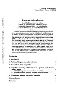
If the label was even (i.e. i0 = 0) then the value is halved and if it was odd (i0 = 1) then the cycling of i0 to the leading position adds 2m−1 and the residual even part is halved. This cycling may be physically achieved by m − 1 state swaps, of qubits 0 and 1, then 1 and 2 etc. up to qubits m − 2 and m − 1. Alternatively we may just reorder the output wires as shown in figure 1 below. 0

0

1

1 F T2m

2 .. .

EQUALS:

2 .. .

m−1

m−1

0

×

1

C1

2

×

×

H

C2

.. .

F T2m−1

.. .

m−1

Cm−1

C C

0 C

C## #C C C C C C CC

1 .. . m−2 m−1

Figure 1. The network diagram for the decomposition of F T2m into F T2m−1 and O(m) extra operations. The conditional phase shift Cp on the pth qubit is denoted by a box on the pth qubit line and a connection across to the 0th qubit with a cross to denote the fact that its operation on the pth qubit is “controlled” by the requirement that the 0th qubit have value 1. Iterating this construction for F T2m−1 in terms of F T2m−2 etc. yields the standard network for the fast Fourier transform on Z2n as given for example in [10]. If Q(2m ) denotes the number of operations needed to implement F T (2m ) in the quantum context then the above description shows that Q(2m ) = Q(2m−1 ) + O(m)

12

giving Q(2n ) = O(n2 ) This quadratic time quantum algorithm for F T (2n ) is used in Shor’s factoring algorithm [10, 13].

Utility of the Fourier Transform The utility of the Fourier transform F in the algorithms of Deutsch, Simon and Shor [6, 8, 9] has been described in [13]. We will here outline in general terms, its fundamental application to the determination of periodicities. A different interpretation of F in terms of the problem of phase estimation, has been given in [22]. Let f : G → X be a function on the group (taking values in some set X) and consider K = {k ∈ G : f (k + g) = f (g) for all g ∈ G}

K is necessarily a subgroup of G called the stabiliser or symmetry group of f . It characterises the periodicity of f with respect to the group operation of G. Given a device that computes f , our aim is to determine K. More precisely we wish to determine K in time O(poly(log |G|)) where the evaluation of f on an input counts as one computational step. (Note that we may easily determine K in time O(poly(|G|)) by simply evaluating and examining all the values of f ). We begin by constructing the state 1 X |f i = q |gi |f (g)i |G| g∈G

and read the second register. Assuming that f is suitably non-degenerate – in the sense that f (g1 ) = f (g2 ) iff g1 − g2 ∈ K i.e. that f is one-to-one within each period – we will obtain in the first register 1 X |g0 + ki (18) |ψ(g0 )i = q |K| k∈K corresponding to seeing f (g0 ) in the second register and g0 has been chosen at random. In eq. (18) we have an equal superposition of labels corresponding to a randomly chosen coset of K in G. Now G is the disjoint union of all the cosets so that if we read the label in eq. (18) we will see a random element of a random coset, i.e. a label chosen equiprobably from all of G, yielding no information at all about K. The Fourier transform will provide a way of eliminating g0 from the labels which may then provide direct information about K. Consider the basis {|χg i : g ∈ G} of shift invariant states introduced in eq. (6). Next note that the state in eq. (18) may be written as a g0 -shifted state: X

k∈K



|g0 + ki = U(g0 ) 

X

k∈K

13



|ki

Hence if we write this state in the basis {|χg i , g ∈ G} then k |ki and k |g0 + ki will contain the same pattern of labels, determined by the subgroup K only. According to eq. (7) the Fourier transform converts the shift-invariant basis into the standard basis. Thus after applying F to eq. (18) we may read the shift-invariant basis label by reading in the standard basis, yielding information about K. In terms of the presentation of G given in eq. (8) and the associated formulas for the irreducible representations given by eqs. (10) and (11) we may compute explicitly the pattern of labels associated with a subgroup K ⊂ G. As an example consider G = Zmn and K = mZ = {0, m, 2m, . . . , (n − 1)m} with |K| = n. Then the Fourier P transform of the fundamental periodic state |Ki = √1n k∈K |ki is P





1 XX F |Ki = √ χl (k) |li n m l∈G k∈K

P

(19)

Thus the labels appearing are precisely those l ∈ Zmn for which X

k∈K

χl (k) 6= 0

(20)

To sort out this condition we introduce a further elementary property of irreducible representations. For any group G the constant function χ(g) = 1 for all g ∈ G, is clearly an irreducible representation (the trivial representation) and using the orthogonality property (B) between χ and any other irreducible representation χ′ we see that X χ′ (g) = 0 g∈G

Now χl restricted to the subgroup K is an irreducible representation of K so eq. (20) can hold if and only if χl (k) = 1 for all k ∈ K According to eqs. (10) and (11) we have χl (k) = exp 2πi

cl kl = exp 2πi mn n

where we have introduced c using the fact that k = cm is always a multiple of m, by definition of K. This will equal 1 for all c = 0, . . . , (m − 1) if and only if l is a multiple of n i.e. l = 0, n, 2n, . . . , (m − 1)n. Thus the pattern of labels associated with mZ ⊂ Zmn is nZ and furthermore in eq. (19) each such label will appear with equal amplitude √1m . A similar calculation for the subgroup {0, ξ} ⊂ (Z2 )n (where ξ is a chosen n-bit string) shows that the resulting pattern of labels, after applying the Fourier transform for (Z2 )n to the periodic state √12 (|0i + |ξi), is {ν : ξ · ν = 0}. This 14

fact forms the basis of Simon’s algorithm [8, 13, 23].

Conclusion Let |ψi be an n-qubit entangled state and U a 1-qubit unitary operation.We have seen that the one-step physical operation of applying U to (say) the first qubit of |ψi corresponds to a state transformation which generally requires an exponential (in n) effort to compute classically. Indeed mathematically the transformation is represented by a tensor product U ⊗ I2 ⊗ . . . ⊗ I2 (where I2 is the 2 by 2 identity matrix, which represents the operation of “doing nothing” on the corresponding qubits). The tensor product spreads the effect of U into an exponentially large matrix. Stated otherwise, we can say that the physical operation of doing nothing to a subsystem of an entangled system is a highly nontrivial operation and gives rise to an exponentially enhanced information processing capability (when performed in conjunction with some operation on another small part of the system). We have given an analysis of the implementation of the fast Fourier transform algorithm in a quantum context and shown that its exponential speedup (as compared to the corresponding classical computation) derives wholly from the above tensor product property. We have also given a general discussion of the role of entanglement in quantum computation and the utility of the Fourier transform in the known quantum algorithms.

Acknowledgements This work was supported in part by the European TMR Research Network ERBFMRX-CT96-0087 and the National Institute for Theoretical Physics at the University of Adelaide.

References [1] Feynman, R. P. (1982) Int. J. Theor. Phys. 21, 467. [2] Deutsch, D. (1985) Proc. Roy. Soc. London Ser. A 400, 97. [3] Holevo, A. S. (1973)Probl. Inf. Transm. 9, 177. [4] Fuchs, C. and Peres, A. (1996) Phys. Rev. A. 53, 2038-2045. [5] Cover, T. and Thomas, J. (1991) “Elements of Information Theory”, John Wiley and Sons. [6] Deutsch, D. and Jozsa, R. (1992) Proc. Roy. Soc. London Ser A 439, 553-558.

15

[7] Bernstein, E. and Vazirani, U. (1993) Proc. 25th Annual ACM Symposium on the Theory of Computing, (ACM Press, New York), p. 11-20 (Extended Abstract). Full version of this paper appears in S. I. A. M. Journal on Computing 26 (Oct 1997). [8] Simon, D. (1994) Proc. of 35th Annual Symposium on the Foundations of Computer Science, (IEEE Computer Society, Los Alamitos), p. 116 (Extended Abstract). Full version of this paper appears in S. I. A. M. Journal on Computing 26 (Oct 1997). [9] Shor, P. (1994) Proc. of 35th Annual Symposium on the Foundations of Computer Science, (IEEE Computer Society, Los Alamitos), p. 124 (Extended Abstract). Full version of this paper appears in S. I. A. M. Journal on Computing 26 (Oct 1997) and is also available at LANL quant-ph preprint archive 9508027. [10] Ekert, A. and Jozsa, R. (1996) Rev. Mod. Phys. 68, 733. [11] Kitaev, A. (1995) “Quantum Measurements and the Abelian Stabiliser Problem”, preprint available at LANL quant-ph preprint archive 9511026. [12] Jozsa, R. (1997) “Entanglement and Quantum Computation” in Geometric Issues in the Foundations of Science eds. S. Huggett, L. Mason, K. P. Tod, S. T. Tsou and N. M. J. Woodhouse (Oxford University Press). [13] Jozsa, R. (1998) Proc. Roy. Soc. London Ser A, 454 323-337. [14] Fraleigh, J. B. (1994) A First Course in Abstract Algebra, 5th edition, Addison Wesley Publishing Company. [15] Cooley J. W. and Tukey, J. W. (1965) Math. Comp. 19, 297. [16] Gauss, C. F. (1886) Theoria interpolationis methodo nova tractata, Gauss’ collected works volume 3. [17] Maslen, D. K. and Rockmore, D. N. (1995) Generalised FFT’s – a Survey of Some Recent Results, in Proc. DIMACS Workshop on Groups and Computation – II. [18] Grover, L. (1996) Proc. 28th Annual ACM Symposium on the Theory of Computing, (ACM Press, New York), p. 212-219. [19] Papadimitriou, C. H. (1994) Computational Complexity (Addison-Wesley, Reading, MA).

16

[20] Fulton, W. and Harris, J. (1991) “Representation Theory – A First Course”, chapters 1 and 2, (Springer Verlag). [21] Hoyer, P. (1997) “Efficient Quantum Algorithms”, preprint available a quantph/9702028. [22] Cleve, R., Ekert, A., Macchiavello, C. and Mosca, M. (1998) Proc. Roy. Soc. London Ser A, 454, 339-354. [23] Brassard, G. and Hoyer, P. (1997) An exact polynomial-time algorithm for Simon’s problem. Preprint, available at http://xxx.lanl.gov as quant-ph/9704027.

17