picture of quantum mechanics.4-'0 The former stress the differences ... (1) The lack of a universally accepted definition of quantum chaos and the lack of ...
Quantum
chaos: An entropy
approach
Wojciech SXomczyriski Instytut Maternavki, Uniwersytet Jagielloliski, ul. Reymonta4, 30-059 Krakdw, Poland Karol iyczkowski Instytut Fizyki, Uniwersytet Jagielloliski, ul. Reymonta4, 30-059, Krakdw, Poland (Received 18 January 1994; accepted for publication 8 April 1994) A new definition of the entropy of a given dynamical system and of an instrument describing the measurement process is proposed within the operational approach to quantum mechanics. It generalizes other definitions of entropy, in both the classical and quantum cases. The Kolmogorov-Sinai (KS) entropy is obtained for a classical system and the sharp measurement instrument. For a quantum system and a coherent states instrument, a new quantity, coherent states entropy, is defined. It may be used to measure chaos in quantum mechanics. The following correspondence principle is proved: the upper limit of the coherent states entropy of a quantum map as h-+0 is less than or equal to the KS-entropy of the corresponding classical map.
“Chaos umpire sits, And by decision more imbroils the fray By which he reigns: next him high arbiter Chance governs all. ” John Milton, Paradise Lost, Book II 1. INTRODUCTION Quantum chaoslY2is a controversial subject. Some physicists regard it as a theory, established to such an extent that it may be presented to the general audience.3 Others treat it merely as “a new style in Emperor’s clothing” and seem to doubt the possibility of fitting it into the present-day picture of quantum mechanics.4-‘0 The former stress the differences between quantum systems with classical chaotic and regular counterparts such as, for instance, the type of the distribution of nearest-neighbor energy level spacings, which can be Poisson or skew normal (Wigner), respectively. The latter believe that no quantum time evolution can be recognized as chaotic if one looks at the problem from the algorithmic complexity theory point of view, which they regard as the most relevant to the case. Indisputably, two problems seem to be open and, in a sense, embarrassing (see also Refs. 11 and 12): (1) The lack of a universally accepted definition of quantum chaos and the lack of quantities which may be used to measure chaos, such as entropy or Lyapunov exponents in the classical case. (2) An inconsistency with the Correspondence Principle: classical chaotic systems and their quantum mechanical counterparts seem to show qualitatively different behavior, even in the limit as h-+0. In the present paper we put forward a rigorous mathematical framework to discuss and, hopefully, solve these problems. Let us start from some general considerations. Ford4 posed the following basic question: What is chaos and what does it mean? We believe that the most fundamental feature of a chaotic system is unpredictability. The precise mathematical meaning of this word may be given within the algorithmic complexity theory or the information theory. However, even if we consent to this
5674
J. Math. Phys. 35 (ll),
November 1994
0022-2466l94l35(11)l5674/27/$6.00 Q 1994 American Institute of Physics
Downloaded 21 Nov 2001 to 128.8.92.79. Redistribution subject to AIP license or copyright, see http://ojps.aip.org/jmp/jmpcr.jsp
W. SIomczyriski and K. &czkowski:
Quantum chaos: An entropy approach
5675
definition, the following question still remains: What are the quantities whose evolution we try in vain to predict? Two possible answers should be considered: unpredictability may concern either the states of the system or the outcomes of a measurement. Even though evidently connected with one another, these two approaches do not coincide. The difference is less important in the classical case, where we can, at least theoretically, measure the state of a system (e.g., the positions and momenta of classical objects) with an arbitrary accuracy and assume that the process of measurement does not alter the dynamics of the system. However, even in that case, the methods of extracting the entropy or the Lyapunov exponents from the equation of motion and from the analysis of the data (the time series) differ considerably. They are, nevertheless, believed to lead to the principally identical results. In the quantum case the situation is entirely different. The time evolution of the states of a given quantum system described in the simplest case by wave functions is almost periodic and thus predictable, at least for finite particle number, spatially bounded and undriven quantum system.4~5~7~8 In contrast, successive outcomes of a measurement can form chaotic and unpredictable sequences, and, as we see further, they really do! One can object to the former approach (as Ford did), distinguishing between intrinsic quantum chaotic behavior and chaotic behavior occurring in a quantum system due to interactions with classical measuring devices. However, “intrinsic quantum chaos” is a rather vague notion, and, if we subscribe to Ford’s point of view as to a general rule, we might be forced to classify one and the same system once as regular and another time as chaotic, depending on the particular mathematical framework we used. For instance, we can describe the dynamics of a classical mechanical system as the evolution in the phase-space governed by the canonical equations of motion or as the evolution in the space of smooth densities governed by the Liouville equation. Now, if we consider any mixing system, e.g., the geodesic motion of a mass point on a compact surface of negative curvature or the Arnold cat map, it becomes evident that the chaotic and unpredictable behavior of point trajectories coexists with a regular and predictable behavior of densities, which tend weakly to the uniform density (see, however, Ref. 6). Quantum mechanics yields another example. As we have already remarked, the time evolution of a quantum state may be described by Schrijdinger equation, which is linear and so, in a sense, leads to predictable dynamics. However, the same system can be equivalently described by the equations of Bohmian mechanics, which are nonlinear, and hence admit any kind of chaotic behavior (see Ref. 13 and Ref. 14, $6.10.2). Summing up-we believe that the approach linking chaos with the unpredictability of the measurement outcomes is the right one in the quantum case (see also Ref. 12). In order to measure this unpredictability we introduce the notion of entropy, which generalizes other definitions, in both the classical and quantum case. Several attempts to introduce the notion of entropy into quantum mechanics have been made,11V’5-39however, none of them might be applied to define quantum chaos rigorously. In this work we try to bridge the gap by introducing a new definition of quantum entropy based on coherent states. This entropy is a function of the entire dynamical system and the measurement process. Hence, it should be distinguished from von Neuman entropy’7’29 given by -Tr p In p, which describes the properties of a single state p, and from Ingarden-Urbanik entropy (A-entropy), which describes the properties of a quantum state after a single measurement.15 The chief points of the general framework for the study of quantum chaos we would like to propose are the following. (1) The notions of chaos and regularity may be attributed to the pair consisting of a quantum system and an instrument measuring an observable, rather than to the quantum system alone. (2) We assume that a large number of successive measurements are performed on the evolving system by means of the measuring instrument and that the motion of the system is perturbed by the measurement process. Then the complete dynamics can be described by a quantum stochastic process (QSP). In special cases the process is Markovian and the evolution of the measurement outcomes can be described by a Markov operator.
J. Math. Phys., Vol. 35, No. 11, November 1994
Downloaded 21 Nov 2001 to 128.8.92.79. Redistribution subject to AIP license or copyright, see http://ojps.aip.org/jmp/jmpcr.jsp
5676
W. Sfomczyriski and K. iyczkowski:
Quantum chaos: An entropy approach
(3) For the quantum stochastic process we define a non-negative quantity, quantum entropy, which evaluates the degree of randomness of the sequences of the measurement outcomes. We propose the division of quantum entropy into two components: quantum measurement entropy and quantum dynamical entropy. Each of them measures a different kind of randomness: the first, that coming from the process of measurement, and the second, that connected with the underlying dynamics of the system. (4) To compare the behavior of quantum mechanical systems and their classical counterparts we study the combined dynamics arising as a result of the interaction between the evolving quantum system and the generalized coherent states instrument which is related to an approximate or fuzzy measurement in quantum mechanics.40-42The distribution of the outcomes of the measurement performed by means of this instrument is the generalized Husimi representation of the state of the system at the instant after the measurement. The QSP associated with the combined evolution of the system repeatedly measured by this apparatus is Markovian and the corresponding Markov operator has a smooth kernel. We call quantum entropy connected with this QSP the coherent states quantum entropy or, briefly, C&quantum entropy. Its dynamical component may be used to measure the degree of the stochasticity connected with the unitary dynamics and positivity of this component may be accepted as a rigorous definition of quantum chaos. Loosely speaking we can say that the quantum system is ‘chaotic if the unitary dynamics produces some additional unpredictability beyond that induced by the measurement process. We try to quantify this idea by introducing dynamical CS-entropy. (5) We apply the results of the theory of random perturbations of dynamical systems43to state the correspondence principle for entropy. Omitting several technical assumptions, it can be expressed as follows: The upper limit of the CS-quantum entropy of a quantized classical dynamical system as h--+0 is less than or equal to the Kolmogorov-Sinai (KS) entropy of this system. We conjecture that if the classical dynamical system is hyperbolic and transitive (e.g., the cat map), then the CS-quantum entropy in question gives the KS entropy of this system in the semiclassical limit (r&+0). (6) In several cases [e.g., for SU(N) coherent states] we can show that measurement CS-quantum entropy tends to zero as h--+0. Then the correspondence principle also holds for the dynamical CS-quantum entropy. In other words, in this case, the two limits, the time limit (t--+m) and the semiclassical limit (h-+0), may commute. This feature differs considerably our model from other approaches to the notion of quantum entropy. The present paper is organized in the following way. In Sec. II we recall the basic facts of the operational approach to quantum mechanics. Since in our description of quantum chaos we take into consideration the measurement process and want to compare classical and quantum systems, the operational approach seems to be the most natural and convenient one. In Sec. III we introduce quantum entropy, quantum measurement entropy, and quantum dynamical entropy, study their properties and compare our definition with other concepts of entropy existing in the literature. In Sec. IV we analyze in detail quantum entropies connected with generalized coherent states instruments which seem to be the most important from “quantum chaotic” point of view. In Sec. V we show how to formulate the corresponding principle for entropy, applying the results of the theory of random perturbations of dynamical systems. In Sec. VI we illustrate our approach by an example of a quantized classical map on the sphere S2. Finally, Sec. VII contains concluding remarks and a list of open problems.
J. Math. Phys., Vol. 35, No. 11, November 1994
Downloaded 21 Nov 2001 to 128.8.92.79. Redistribution subject to AIP license or copyright, see http://ojps.aip.org/jmp/jmpcr.jsp
W. SIomczyriski and K. iyczkowski:
II. OPERATIONAL
APPROACH
TO QUANTUM
Quantum chaos: An entropy approach
5677
MECHANICS
The operational approach to quantum theory was developed in an axiomatic form by many authors in the late 60s and early 70s. In this section we mainly follow Davies and Lewis’ formulation,44-46 partially suited to our needs. Their approach seems to be broad enough to cover all the applications we refer to. Nevertheless, one could also use the more general approach of Gudder47 based on the notion of a convex structure or the approach based on the general theory of measurement in quantum mechanics.48,49 A. State space
and phase
space
We define a state space as a pair ( V, K), where (9 (ii) (iii) (iv)
V K if if
is a real Banach space with the norm 1111; is a closed cone in V; U,U E K, then ~(ull+llull=llu+ull; u E V and 00, then there exist U~,U~E K such that u=u1-u2
and Ilulll+Ilu211 sW6. Then oYZ are just the canonical coherent states. We can construct an instrument 9 as in example (E) taking fi=W6, m the Lebesgue measure divided by 27r and P,,= ILY,J(cY,,~I for (y,z) EWE. Then the marginal observables of xJ defined by x,(E)=x,AEXR) andX2(F)=X,A(RXF), for E,F EB(W), are the approximate position and momentum observables. The respective POV measures are given by the convolutions,46*56 namely At(E) = (xE*l~ul~)(Q) andAz(F) = (xF*l&12)(P) for E,FeB(W), where ,&. denotes the characteristic function of a set G, for G EB(B), and & stands for the Fourier transform of the function cr. The map (y,z)+?,(y,z) =(c~,,~lpIc~,,~) is the ordinary Husimi distribution57*58 (or Q function) of the state p. This function has become recognized as extremely useful for the analysis of quantum chaos.59-64 Analogously, we can construct an instrument simultaneously measuring approximate momentum and position observables in the reduced phase space (cylinder or torus) or different spin components observables, where the phase space is the sphere. For this purpose, one should use the appropriate vector coherent states,64’65as it is demonstrated in Sec. VI. (G) Classical mechanics: sharp and approximate measurements -Let X,V,K be as in example (A) and let (fi,z)=(X,B(X)), where B(X) o-algebra of X. Then 3 given by RE)P~A)=P~(A~E),
is the Bore1
(6)
for p E V and A, E E 2, is an instrument describing the sharp classical measurement. The corresponding observable has the form x.AE)P=AE),
(7)
for E E c and PE V. This measurement is nondemolition, i.e., Y(fl)p=p for each PE V. In order to show how one can model an approximate (or unsharp) classical measurement, we consider the following example. Let X=W3 and let J’Y be a three-dimensional normal distribution with the zero mean. Then the instrument Ygiven by
for A, E E Z and ,Y E V with the observable
x:dE)~= I EOW4b)dr
(9)
describe a measurement in question.
J. Math. Phys., Vol. 35, No. 11, November 1994 Downloaded 21 Nov 2001 to 128.8.92.79. Redistribution subject to AIP license or copyright, see http://ojps.aip.org/jmp/jmpcr.jsp
5680
W. Sfomczyhski and K. iyczkowski:
Quantum chaos: An entropy approach
(H) Nuclear instruments -Cycon and Hellwig showed that many important instruments can be constructed in the following way (see also Refs. 67 and 68). Let (V,K) be a state space, let (fl,C) be a phase space, and let x be an observable. Let us take an x-measurable, x-essentially bounded state valued map $:R-+V. Then the formula Y(E)=
I
E4dx,
for EEIZ,
(10)
defines an instrument. Cycon and Hellwig called such an instrument nuclear. The integral in the formula is, so called, (x)-integral. For the definition of x-measurability, x-essential boundedness, and (x)-integral consult the Appendix in Ref. 66. Note that x2=x and Y(E)u = J&dx( . )u for all EEzanduEV. (J) Absolutely continuous nuclear instruments -Let V, K, a, 2, and x be as in the previous example. Let m be a measure on (fi,c). Then x is absolutely continuous with respect to m (see Ref. 42), if there exists a measurable map f:fi+g such that So f dm = r and x(E) = SEf dm for each E E’C. Then, the nuclear instrument from example (H) has a particularly simple form:
(11) for E E 2 and u E V. We call 9 an absolutely continuous nuclear (ACN) instrument. Here, we can interpret f(a)u as the “transition probability density” from a state u to a measurement outcome a and &a) as the state of the system after the measurement if the value a has been observed. Ozawa67*68and Brachielli and Belavkin69 called d(o), where w~fi, an “a posteriori state.” for We shall say that 3’ is informationally complete42 if u=w, whenever f(b)u=f(b)w almost every b (with respect to m). The instruments considered in examples (D) and (E) are ACN instruments, if projections {PalaEn are atomic, i.e., rank P,= 1 for all a E a. This follows from the equality tr( Pp) P = PpP valid for every atomic projection P and psfi%). In this case f(a)p=flp(a)=tr(P,p) and +(a) = P, . Hence, a generalized coherent states instrument is informationally complete, if each density operator is uniquely determined by its generalized Husimi distribution. This is true, e.g., for canonical coherent states and spin coherent states.51The instrument 3’ described in example (G) is also an ACN instrument with f(y)p = (~V*p)(y) and #(y) =&j , for y EBB and pc V, where “y; is the normal distribution ./t“ translated by the vector y. (K) Transformed instrument -Let (V,K) be a state space and let (0,x) be a phase space. Let us consider an isometric automorphism T: V-+ V and an instrument 9?$-& The formula .FT( E) : = T- ‘oY( E)oT,
02)
for E E 2, defines a new instrument. We call it a transformed instrument. C. Quantum
stochastic
processes
In this section we assume that (V,K) is a state space, fi is a Polish space (i.e., metric, complete, and separable) and 2 its Bore1 a-algebra. Following Srinivas7’ we can define a quantum stochastic process (QSP) as an arbitrary family of instruments {.Yt}f E%. The parameter “t” may be interpreted as a physical time. Let 2=Z or 2=R, for discrete or continuous time domain, respectively. The finite-dimensional distributions of the process are measures prO ,,,,,f,_, defined on (@,E(fl’)) as the natural extensions of the set functions given by
J. Math. Phys., Vol. 35, No. 11, November 1994
Downloaded 21 Nov 2001 to 128.8.92.79. Redistribution subject to AIP license or copyright, see http://ojps.aip.org/jmp/jmpcr.jsp
W. SJomczyhski and K. ?yczkowski:
u k(),....t”-,(E,X...
Quantum chaos: An entropy approach
XE,-1)=~((~;,_,(E,-1)0~;n_,(E,-2)o...o~O(E~))~),
5881
(13)
where n EN, to12dm(b)-g(h) =o, D7i f&-+0 UEX If x lim sup
(35)
for every continuous function g:X-% The assumption of regularity has the following physical interpretation. The members of the difference in (35) are the quantum expectation value of g in the state u~IL~~) and the classical expectation value of g in the state So,, respectively. Condition (35) is equivalent to the following one (see Appendix E). For each sufficiently small 6>0
I~“~IwfahN2dm(b)=1. h-+0sexI B(Oa.6) Dh lim inf
(36)
Simple interpretation of the above condition is shown in Fig. 1. In the sequel we shall assume that the quantization procedure is regular. measurable partition of X such that be a finite Let JA={E, ,...,Ek} m (06) =m (U “= t a( Ei)) = 0. Let Yh be the coherent states instrument connected with the family of coherent states {I LYE): a E X}. We assume that ph is a stationary state for the combined evolution given by the operator Uh and the generalized coherent states instrument Yfi, such that the generalized Husimi distribution Qp, = 1, e.g., p,,= (l/D& .I [if 9’h is informationally complete this is the only possible choice-see Proposition 2(A) and (B)]. We can now formulate our main result. Correspondence principle for quantum entropy:
FIG. 1. Regular quantization. Procedure linking a family of quantum maps {VA} with a classical map 0 is regular, if the integral of the Husimi distribution Q of the transformed coherent state LI*I ai) taken over a ball of an arbitrary small radius 6, localized at the classical image @a of an element a of the phase space X, tends in the semiclassical limit to the unity, uniformly with respect to a.
J. Math. Phys., Vol. 35, No. 11, November 1994
Downloaded 21 Nov 2001 to 128.8.92.79. Redistribution subject to AIP license or copyright, see http://ojps.aip.org/jmp/jmpcr.jsp
W. SIomczyriski and K. iyczkowski:
Quantum chaos: An entropy approach
lim sup H(U~,~~,-~,P~~)~H(OI~)~H(O), R-+0
5689
(37)
where H(O) denotes the KS-entropy of the classical map 0. To prove the above result it suffices to use the appropriate theorems on entropy of random perturbations of dynamical systems. See Appendix F for details. The fact that the CS-quantum entropy is bounded in the limit as h+O by KS-entropy does not contradict Remark 6, as the limits k-+a and fL+O do not commute. Moreover, we believe that the following conjecture, analogous to the Kiefer’s “entropy via random perturbations” theorem,43*74is true for a broad class of classical maps and theirs quantizations. Conjecture 2: IfX is a smooth compact manifold and 0 is a C2 hyperbolic transitive difseomorphism of X, then there exists E>O such that diam(A)Se implies (38)
lim WU~,,~,S,&~=H(@),
fr-+O
where diam(,&:=max(diam(~J,...,diam(~~)). Remark 8: In condition (36) one can use an arbitrary metric on the compact space X. Note, however, that a family of coherent states itself generates a Riemannian metric on X. See Refs. 50 and 54 for the general case and Ref. 89 for the SU(iV) coherent states. In the latter paper the Riemannian metric is given by the logarithm of the modulus of the coherent states overlap. Vi. EXAMPLE-W(S)
COHERENT
STATES
In order to illustrate the definition of quantum entropy we discuss classical systems with the phase space homeomorphic to the two-dimensional sphere S2. Due to compactness of the phase space, the Hilbert space .%Y,.,describing the corresponding quantum dynamics is finite dimensional. Consider three components {J, ,J, ,J,} of the angular momentum operator J. These operators are related to the infinitesimal rotations along three orthogonal axis {x,y,z} in R3 and fulfill the standard commutation relation
CJk, Jd= iEk[,,J,,
(39)
,
where k,l,n=x,y,z and ek,,, represents the antisymmetric tensor. Operators J, = J,I!I iJ and J, are generators of the SU(2) group. Eigenvalue j( j + 1) of the Casimir operator i’= Jz + J! + 5: determines the dimension N= 2 j + 1 of the representation of the group. Since the semiclassical limit is obtained by letting j-m, an integer or half-integer quantum number j might be considered as proportional to jL-l. Common eigenstates Ij,m), m = -j ,...,j of the operators J2 and J, form an orthonormal basis in .%$,,. It is convenient to choose as a reference state the state lj,j) (of maximal weight) and to define the SU(2) coherent state?’ by
Ij,y)= m
WrJ-llj,j),
(40)
where y is an arbitrary complex number. These coherent states (CS) can be expanded in the eigenbasis of J2 and J, as53
m=j Ij,y)=@iT C 3j-m(l+yy)-i j?m m=-j
Ij,m). ii . II”’
A stereographical projection y tan(??/2)exp( icp) links a coherent state 1j, y) = 1j, 8, cp) to a point (4,(p) on the sphere S2. Note that S2 is isomorphic to the coset space SU(2)/U(l), where U(1) is the maximal stability subgroup of SU(2) with respect to the state 1j,j), i.e., the subgroup of all
J. Math. Phys., Vol. 35, No. 11, November 1994
Downloaded 21 Nov 2001 to 128.8.92.79. Redistribution subject to AIP license or copyright, see http://ojps.aip.org/jmp/jmpcr.jsp
5690
W. SIomczyriski and K. iyczkowski:
Quantum chaos: An entropy approach
elements of SU(2) that leave lj,j) invariant up to a phase factor. Hence the above construction may be treated as a particular case of the general construction of group-theoretic coherent states52’54’90 and, in consequence, as a particular case of our examples (E) and (M). The appropriate instrument describes unsharp simultaneous measurement of different spin components.65’91We introduce the factor dm in formulas (40) and (41) in order to ensure the coherent states identity resolution in the form (42) where the Riemanian measure p on S2 is given by dp=sin 8d6dcpl4 rr and so does not depend on the quantum number j. This enables the respective Husimi distribution of the coherent states to tend to the Dirac &function as fit0 (j-+m). Expectation values of the components of J are (j,S,cpIJlj,4,q)=j(2j+
l)(sin6
coscp, sin8 sincp, cos6)
(43)
and justify the interpretation of CS as vector states oriented along the direction defined by a point on the sphere.53’54*90 Similar formulas written in the complex number representation (i,rlJ,lj,r)=j(2j+l)(l-yy)l(l+yy)
(4-4
and (jTdJ-b,y)=2jt2j+
l>y/tl+
~$3
(45)
allow us to obtain the relation (46) Consider now a unitary operator U governing the quantum dynamics in a (2 j + 1)-dimensional Hilbert space. In the analogy to the identity (46) we define a family of classical maps by (jTdUtJ-Ub,y)
0i(y)= Letting j+m
j(2j+l)+(j,yIUtJ,Ulj,y)’
(47)
we may obtain a classical map on the complex plane @(r)=;l~
@j(Y)?
(48)
if the limit exists. Applying the stereographical projection we find a classical map @:S2+S2, which corresponds to the map O:C+C. The above method of assigning classical maps to a quantum dynamics built by SU(2) operators may be easily generalized92 to group SU(N), with Na3. Let us examine the following simple example. Consider an operator describing the rotation along the z axis by the angle K: U,=exp(iKJ&
(49)
Inasmuch as any CS]j,i?,,cp) is transformed into the rotated CS U~lj,~,cp)=lj,6,cp+K),
(50)
J. Math. Phys., Vol. 35, No. 11, November 1994
Downloaded 21 Nov 2001 to 128.8.92.79. Redistribution subject to AIP license or copyright, see http://ojps.aip.org/jmp/jmpcr.jsp
W. SIomczyriski and K. .?yczkowski: Quantum chaos: An entropy approach
5691
formula (47) does not depend on the quantum number j and leads to the classical map given by
or (52) Please note that there exist several other quantum operators corresponding to the same classical map in the sense of (47) and (48); one of the simplest might be written in the form
where X is a finite parameter and J, is an arbitrary component of the operator J. Quantum map (49) transforms the coherent state p,Zl,,so)into ~,~(&,cp>). In order to verify validity of the condition (36) we calculate an integral over the circle of radius S centered at G(lY,fp):
I B(Q(W,6)
I(~~~‘~~‘I~~l~~~~cp)12 sin 6’ d6’dq’ = 1 - [cos( S/2)]4j+2. 2jf
1
(54)
The above result does not depend on the initial point of the phase space (IY,~) and shows that in the semiclassical limit j--+a the Husimi distribution of the quantum state Utlj, 4,(p), integrated over a circle centered at the point o(rY,;cp) of an arbitrary small radius 00, tends uniformly to the unity. Requirement (36) is therefore fulfilled and the procedure of quantization linking the quantum map (49) with the classical map (52) is regular. Hence it is possible to apply to this case the correspondence principle for entropy (37). Classical map (52) describes an integrable system and is characterized by zero KS-entropy. It follows,.therefore, that the quantum CS-entropy of the map (49) tends to zero in the limit j--+a. Quantum map (49) can be easily generalized by admitting another unitary term parametrized by E: U3 = eXp( i d,)eXp(
i eJz/j).
(55)
This operator describes dynamics of the periodically kicked quantum top.93-95 For sufficiently large values of K and E the classical analogue of this model displays chaos (the KS-entropy is positive96) and thus might serve for further study on coherent states quantum entropy. Setting the angle K to zero in the map (49) we obtain the identity operator U = I and may calculate the entropy H,, , which measures the randomness caused by a series of measurements performed by SU(2) coherent states instrument. Due to correspondence principle (37) we have lim H,,=O. h-+0
Preliminary results indicate97 that H,,
VII. CONCLUDING
tends to zero asymptotically as - (In h) &.
REMARKS
We have proposed a general definition of the entropy of a dynamical system equipped with the measuring device. For a classical system and the sharp measuring instrument we obtain the Kolmogorov-Sinai entropy, which can be used to define classical chaos. Entropy of quantum system depends significantly on the way the process of a measurement (necessary to gain an information about the quantum dynamics) is performed.
J. Math. Phys., Vol. 35, No. 11, November 1994
Downloaded 21 Nov 2001 to 128.8.92.79. Redistribution subject to AIP license or copyright, see http://ojps.aip.org/jmp/jmpcr.jsp
5692
W. SIomczyliski
and K. iyczkowski:
Quantum chaos: An entropy approach
Our approach covers older definitions of Pechukas-Beck-Graudenz20,30 (where the measuring device is the Liiders-von Neumann instrument) and of Helton-Tabo?’ as the special cases. The other case corresponding to an approximate measurement of quantum observables (described by the coherent states instrument) is of a particular importance. Since the transition function used to describe the successive outcomes of this measurement has the well-defined semiclassical limit, the coherent states quantum entropy is related to the classical Kolmogorov-Sinai entropy. We have proved that the upper limit of the coherent states entropy as fi-+O is less than or equal to the Kolmogorov-Sinai entropy and we conjecture that the equality holds if the underlying classical system is sufficiently chaotic. Two sources of randomness in our model (one coming from the measurement process and the other arising from the dynamics of the system) are separated by dividing the coherent states entropy into the measurement and the dynamical components. We believe that the dynamical coherent states entropy can be used to define and to measure quantum chaos. Note, however, that this quantity depends on the time between successive measurements and on the partition of the phase space. The character of this dependence requires a detailed study. We hope that our work will be a starting point for further investigations in the subject. Hence we would like to point out some open problems that seem to be crucial for a better understanding of CS-quantum entropy. (1) Prove Conjectures 1 and 2 from the present paper. It may happen that the conjectures are false as stated and some additional assumptions are needed. (2) Analyze dependence of CS-quantum entropy (and dynamical CS-quantum entropy) on the time interval between two successive measurements (we expect that it is nonlinear) and on the partition of the phase space. (3) Study dependence of CS-quantum entropy on the choice of the set of coherent states. Note that we may choose different coherent states for a given physical system (e.g., vector coherent states, squeezed states). (4) Calculate the measurement CS-entropy for concrete examples, e.g., for SU(2) coherent states or torus coherent states. (5) Find an example of quantum map with positive dynamical CS-entropy (if Conjecture 2 is true, then any regularly quantized version of a hyperbolic and transitive classical map suits). (6) Examine whether the quantization procedures linking the frequently studied classical models (e.g., baker map, cat map, standard map, periodically kicked top) with their quantum counterparts fulfill the regularity condition (36). Compute analytically or numerically dynamical CS-entropy for these maps. (7) Check which results of the present paper may be generalized to Renyi CS-entropies. Note added in proo$ Pechukas-Beck-Graudenz entropy was studied earlier in the operational setting by Srinivas.*03 His approach coincides with ours when the phase space is finite, but does not cover CS-entropy case. Lindbladlo4 (see also Appendix D) considered a Hilbert space version of Srinivas definition and proved an analog of our Proposition 3 in this situation. Mendeslo5 proposed a definition of quantum entropy that mimics the Brin-Katok’06 approach to KS-entropy. However, he did not discuss the classical limit. ACKNOWLEDGMENTS
It is a pleasure to thank R. Alicki, I. Bialynicki-Birula, M. Capiriski, B. Eckhardt, P Gaspard, I. Guameri, F. Haake, J. Ford, M. Ku& W. A. Majewski, G. Mantica, Ya. Sinai, A. Wehrl, St. Weigert, H. Wiedemann, and T. Zastawniak for stimulating discussions and helpful remarks. We are grateful to Ewa Pawelec for preparing the figure. We also thank an anonymous referee for several valuable comments which helped us to improve our manuscript. Financial support by the project “Kwantowy Chaos” of Polski Komitet Badan Naukowych is gratefully acknowledged.
J. Math. Phys., Vol. 35, No. 11, November 1994
Downloaded 21 Nov 2001 to 128.8.92.79. Redistribution subject to AIP license or copyright, see http://ojps.aip.org/jmp/jmpcr.jsp
W. Sfomczyriski and K. iyczkowski:
APPENDIX
A: PROOF
OF PROPOSITION
Quantum chaos: An entropy approach
5693
1
Setp,(a,b)=f(b)(T,(&a)))andq(u,b) prove the formula
=f(b)(TtOu)
fortE’X,a,bER,anduEV.
Wefirst
by induction on n EN. Let n =O. Applying Eqs. (11) and (14) we obtain (T,(Eo))u=
T-t,,
~Eo(f(~o)~r,o~))dodm(y.) i
= i
~(u,yo)T-r,(~(yo>)dm(Yo), J Eo
642) as required. Assume the formula (Al) holds for n; we shall prove it for n + 1. Applying again (11) and (14) we conclude that the left-hand side of the formula (Al) becomes
(A3) which is, clearly, equal to the right-hand side. It follows from Eqs. (13) and (A2) that (A4) From (13), (Al), and (A4) we obtain
Xdm(yo)...dm(y,-l>dm(y,) =~E~~E~_,~~~~E~~~-~~~,(y,-~~y,)~~~~r,-,o~~o~~~~~~~o~yo~ Xdm(yl>...dm(y,-l>dm(y,),
(A5)
which is a desired conclusion. APPENDIX
B: PROOF
OF PROPOSITION
2
Proof of Proposition 2(A): Let u E V fulfill the condition T(Y(fi)u)=u. Let E EE. Combining (ll),
(Bl)
(17), (20) and (Bl) we obtain
J. Math. Phys., Vol. 35, No. 11, November 1994
Downloaded 21 Nov 2001 to 128.8.92.79. Redistribution subject to AIP license or copyright, see http://ojps.aip.org/jmp/jmpcr.jsp
5694
W. SIomczyliski
and K. iyczkowski:
=
=
Quantum chaos: An entropy approach
f f
Ef(b)(T(4sz)(u)))dm(~)
WI
Ef(@tu)dm@)=&(E),
which was to be shown. Conversely, let u be a stationary state. Then 033)
ff(b)(u)dm(b)=fEf(b)(T(~(n)(U)))dm(b) E
for every E EC. Hence (B4)
f(b)(u)=f(b)(T(~(R)(u)))
for almost every b ~fi (with respect to M). If 3 is informationally complete, (B4) implies (Bl), which completes the proof. Proposition 2(B) follows immediately from (5), (22), and Proposition 2(A). Proposition 2(C) is obvious. APPENDIX
C: GENERALIZED
RliNYI
ENTROPY
Let F, ~6, and u be as in Sec. III and let CSO. We define the R&yi entropy of order LYof F in the initial state u with respect to the partition ,A by the formula75
for a# 1,
(Cl)
where the generalized partition function Za is given by Z”:=
2
(pz
,,,,, n-l(EioX...XEi,_,))a.
(W
rg,...,i,-,=l
Entropy of order 1 is by the definition the generalization of Shannon-Kolmogorov entropy, while entropy of order 0 is called topological entropy (we adopt the convention that O’=O). It is easy to show that Rdnyi entropy is a nonincreasing function of LY.Moreover, the number k of the elements of the partition JA gives the upper bound for the entropy. Namely, Osh”( %‘,JA,u)