Jan 26, 2015 - We will try to give all the mathematical tools needed to a deep understanding of the physics of the. 1. arXiv:1501.06490v1 [math-ph] 26 Jan ...
QUANTUM SYSTEMS WITH TIME-DEPENDENT BOUNDARIES
SARA DI MARTINO Dipartimento di Matematica, Universit` a di Bari, Via Orabona 4
arXiv:1501.06490v1 [math-ph] 26 Jan 2015
Bari, I-70125, Italy PAOLO FACCHI Dipartimento di Fisica and MECENAS, Universit` a di Bari, Via Amendola 173 Bari, I-70126, Italy INFN, Sezione di Bari, Via Amendola 173 Bari, I-70126, Italy
We present here a set of lecture notes on quantum systems with time-dependent boundaries. In particular, we analyze the dynamics of a non-relativistic particle in a bounded domain of physical space, when the boundaries are moving or changing. In all cases, unitarity is preserved and the change of boundaries does not introduce any decoherence in the system. Keywords: Quantum boundary conditions; time-dependent Hamiltonians; product formulae.
1. Introduction We present here the notes of three lectures given by one of us at the International Workshop on Mathematical Structures in Quantum Physics, held in February 2014 in Bangalore at the Centre for High Energy Physics, Indian Institute of Science. The course considers some aspects of quantum systems with time-dependent boundaries, a very active area both from the mathematical point of view, see for instance the works of Yajima [1,2], Dell’Antonio et al [3] and Posilicano et al [4,5], and from a physical perspective. Notable applications arise in different fields ranging from atoms in cavities [6,7] to ions and atoms in magnetic traps [8], to superconducting quantum interference devices (SQUID) [9], to the dynamical Casimir effect in microwave cavities [10]. Moreover, the role and importance of boundary conditions at a fundamental level have been stressed in an interesting series of articles, see [11,12] and references therein, where varying boundary conditions are viewed as a model of space-time topology change. These notes will be organized as follows. In the first lecture, in Section 2, we will study the problem of a quantum particle moving in a one-dimensional box. In particular we will introduce and describe the problem in a pedagogical way focussing on the mathematical aspects of the physical model. We will try to give all the mathematical tools needed to a deep understanding of the physics of the 1
2
S. Di Martino, P. Facchi
problem. Moreover, at the end of the section, we will follow Berry [13] and show how, quite surprisingly, even an easy spectral problem like this can lead to intricate and rich dynamics. In the following lectures, we will look at the dynamical evolution with time-dependent boundaries. In particular, in the second lecture, in Section 3, we will discuss the case in which the walls of the bounding box are moving [14], while in the last lecture, in Section 4, we will look at the problem of the change of boundary conditions with time [15]. Finally, in Section 5 we will draw some conclusions. Interspersed between the lectures we offer a selection of exercises ranging in difficulty. They are useful to focus the attention on specific points and to test the learning of the reader, therefore we kindly recommend not to skip them. 2. Lecture 1: A particle in a one-dimensional box One of the very first problems involving boundary conditions in quantum mechanics is the study of a non-relativistic particle in a one-dimensional box. Indeed, it is one of the exercises sometimes professors give to students just to test their ability. The problem consists in a massive particle moving freely in an infinitely deep well located, say, at I = [a, b] with b > a, from which it cannot escape (Fig. 1).
Fig. 1. A particle moving in a one-dimensional box.
We will see that even if the problem is apparently fairly simple, it leads to very interesting results that stress the difference between classical and quantum mechanics. In fact, the very presence of boundaries in general tends to enhance the quantum aspects of the system. The reason is that in quantum mechanics the behavior at the boundary is constrained by the very structure of the theory and in particular by unitarity. This is at variance with classical mechanics, where the behavior at the boundary does not derive from fundamental principles, and is usually treated phenomenologically. From the mathematical point of view the system is described by a Hamiltonian operator associated to the kinetic energy of the particle, namely the Laplacian, p2 ~2 d2 =− , (1) 2m 2m dx2 acting on square integrable functions (remember that |ψ(x)|2 is a probability denT =
Quantum systems with time-dependent boundaries
3
sity!) with square integrable second (distribution) derivative on the interval I of the box, H2 (I) = {ψ ∈ L2 (I) | p2 ψ ∈ L2 (I)}. In the mathematical literature H2 (I) is known as the second Sobolev space; it is nothing but the maximal domain of definition of the kinetic energy operator T . Equation (1) describes the action of T in the bulk of the box. In order to get a well-defined dynamics, Eq. (1) should be equipped with suitable boundary conditions, which specify the behavior of the particle at the walls. Namely, the wave functions ψ to which we are allowed to apply T must belong to the domain D(T ) = {ψ ∈ H2 (I), with suitable boundary conditions}.
(2)
The question that here arises naturally is how to choose these boundary conditions. This marks the difference between classical and quantum mechanics: in quantum mechanics the behavior at the boundary, encoded in the domain D(T ), derives from basic principles. Indeed, in quantum mechanics the conservation of probability leads to the necessity for the evolution to be represented by unitary operators. But unitarity of the evolution is equivalent to self-adjointness of its generator, as stated in Stone’s theorem [16]: Theorem 1. (Stone) Let (Ut )t∈R be a strongly continuous one-parameter group of unitaries on a Hilbert space H. Then there is a unique self-adjoint operator H on H, called the generator of the group, such that Ut = e−iHt/~ for all t. According to Stone’s theorem the operator T , that generates the dynamics of the particle, Ut = e−iT t/~ , must be self-adjoint, i.e. T = T†
and D(T ) = D(T † ).
(3)
In order to find the domain D(T ) let us consider φ, ψ ∈ H2 ([a, b]); then a double integration by part gives (prove it!): Z b ψ(x)φ00 (x) dx = −hψ 00 |φi + Λ(ψ, φ), (4) − hψ|φ00 i = − a
Λ(ψ, φ) =
ψ 0 (b)φ(b)
− ψ 0 (a)φ(a) − ψ(b)φ0 (b) + ψ(a)φ0 (a).
(5)
The self-adjointness requirement amounts to finding a maximal subspace D(T ) of H2 ([a, b]) on which the boundary form Λ identically vanishes, namely Λ(ψ, φ) = 0 for all φ, ψ ∈ D(T ). The more common boundary conditions you can encounter in the literature are: (1) Dirichlet boundary conditions: ψ(a) = ψ(b) = 0;
(6)
(2) Neumann boundary conditions, involving the derivative of the function: ψ 0 (a) = ψ 0 (b) = 0.
(7)
(Of course, the above conditions must be satisfied by both ψ and φ in the boundary form Λ(ψ, φ)!)
4
S. Di Martino, P. Facchi
Exercise 1. Check that the Dirichlet and the Neumann boundary conditions make Λ identically vanish, and thus, modulo a check of maximality, yield a good domain D(T ) of self-adjointness for the kinetic energy operator T . There is a one-parameter family of boundary conditions that includes Dirichlet and Neumann as limit cases: Robin’s boundary conditions, that connect the function with its derivative at the boundary: ψ 0 (a) = −
1 α tan ψ(a), l0 2
ψ 0 (b) =
1 α tan ψ(b), l0 2
(8)
where α ∈ (−π, π], and l0 is a reference length. From (8) we recover Dirichlet and Neumann in the limits α → π and α → 0, respectively. Notice that the choice of a domain of self-adjointness D(T ) is not just a mathematical nuisance. Different domains give rise to different physics! Indeed, the choice of boundary conditions strongly depends on the physical behavior of the walls, as we will now show. Let us concentrate on one wall, e.g. the left one at a = 0, and look at the scattering process of a plane wave arriving from the left with momentum −~k < 0. After reflection by the wall a plane wave with momentum ~k will arise. Therefore,
-k k
Fig. 2. Reflection at a wall
the wave function will have the form ψ(x) ∼ e−ikx + r eikx ,
(9)
where r is a reflection coefficient. Since we are dealing with an impenetrable box, and we assume that the particle does not stick at the wall, we are forced to require that |r|2 = 1, so that the only freedom left is in choosing a phase, namely r = eiβ . The Dirichlet boundary condition, ψ(0) = 0, corresponds to a phase β = π for all k, while Neumann corresponds to the choice β = 0 for all k. Notice that in general the phase β(k) has a nontrivial dependence on the wavenumber k. The following exercise shows that for a generic α in (8) the behavior of the walls depends on the momentum ~k of the impinging particle through a nontrivial phase β(k). Exercise 2. Prove that Robin’s boundary condition ψ 0 (0) = − l10 tan α2 ψ(0) corre-
Quantum systems with time-dependent boundaries
5
sponds to a momentum dependence of the phase shift β(k) given by tan
β(k) 1 α = tan . 2 k l0 2
(10)
Recover, as a limit, Dirichlet and Neumann, and show that they are the only phases independent of k. The general theory of self-adjoint extensions and boundary conditions [17] asserts that all possible boundary conditions that make T self-adjoint can be parametrized by 2 × 2 unitary matrices U in the following way: i(I + U )Ψ0 = (I − U )Ψ,
U ∈ U(2),
(11)
where � Ψ :=
ψ(a) ψ(b)
� ,
Ψ0 := l0
�
−ψ 0 (a) ψ 0 (b)
� ,
(12)
and I is the identity matrix. Exercise 3. Check that if ψ and φ satisfy (11)-(12) for the same unitary U , then the boundary form (5) vanishes, Λ(ψ, φ) = 0. Robin’s boundary conditions (8) correspond to (prove it!) � −iα � e 0 U = e−iα I = , 0 e−iα
(13)
and in particular the Dirichlet boundary conditions correspond to U = −I, while the Neumann ones are given by U = I. More generally, by taking � −iα � e 1 0 U= , (14) 0 e−iα2 with α1 , α2 ∈ (−π, π] we can describe different boundary conditions at the two endpoints, e.g. Dirichlet/Neumann (α1 = π, α2 = 0), and include all cases considered above, when α1 = α2 . But, of course the unitaries (14) do not exhaust all allowed boundary conditions, since they form only a two-dimensional submanifold U(1) × U(1) of the total four-dimensional manifold U(2). Thus, where do all missing boundary conditions come from? Up to now we have considered only local boundary conditions, somewhat deceived by the physics depicted in Fig. 2: the two walls did not talk each other. Indeed, the unitary matrices in (14) are diagonal and do not mix the boundary values at a with those at b; we missed all nondiagonal unitaries, describing nonlocal boundary conditions. Mathematics tells us that unitarity allows also for them. So what physics do they describe, if any? In fact, nondiagonal unitaries are describing a physical situation which is different from that of a box with two walls far apart. In order to interact, the two ends of the interval should come close, as in Fig. 3, so that the interval should be bent and the two walls should become the two sides of a junction. In other words,
6
S. Di Martino, P. Facchi
Fig. 3. Change of topology: from an interval to a circle
by changing from a diagonal U to a nondiagonal U we are assisting at a change of topology: from an interval to a circle. Therefore, the geometry that is able to support all possible boundary conditions in U(2) is that of a ring with a junction. If the junction is impermeable, i.e. there is total reflection at the walls, we are back to the interval, otherwise there is nonzero transmission across the junction, from one wall to the other. An interesting example is given by the matrix � � 0 e−iα U= = cos α σx + sin α σy , (15) eiα 0 which describes pseudo-periodic boundary conditions (prove it!): ψ(b) = eiα ψ(a),
ψ 0 (b) = eiα ψ 0 (a).
(16)
By passing through the junction, the wave function acquires a phase α. If α = 0 we get the famous periodic boundary conditions, and the geometry is that of a circle; if α = π we get antiperiodic boundary conditions. The phase α encodes the properties of the junction, for example the material it is made of, or its width. In general, if the unitary U has no −1 eigenvalues, the wave function ψ can assume any value at the endpoints of the interval. Only the boundary values of its derivative are constrained in some way. On the other hand, one eigenvalue equal to −1 corresponds to one constraint on the values of ψ at the ends, as for example in the first equation in (16). Finally, two −1 eigenvalues, i.e. U = −I, correspond to two constraints on the boundary values of the wave function, i.e. Dirichlet at both ends. Exercise 4. Prove that the unitary (15) has always an eigenvalue equal to −1. Find its corresponding eigenvector ξ and show that the first equation in (16) is nothing but an orthogonality condition hξ|Ψi = 0. (In Lecture 3 we come back to the geometrical meaning of this condition.) 2.1. Hard walls Let us concentrate now on the textbook case of a particle confined in an infinitely deep well, Fig. 1. The appropriate boundary conditions are Dirichlet’s: ψ(a) =
Quantum systems with time-dependent boundaries
7
ψ(b) = 0. The dynamics of the particle is described by the Schr¨odinger equation i~
∂ψ(x, t) ~2 ∂ 2 ψ(x, t) . =− ∂t 2m ∂x2
(17)
A separation of variables, ψ(x, t) = u(x) exp(−iEt/~), reduces the problem to the solution of the spatial part of the differential equation, that means to find eigenvectors and eigenvalues of the operator T : −
~2 00 u (x) = E u(x). 2m
(18)
The general solution is u(x) = c1 e+ikx + c2 e−ikx ,
(19)
√
with k = 2mE/~ (in principle k can be imaginary, but see below), and c1 and c2 are arbitrary constants that can be fixed (up to a common phase) by imposing the Dirichlet boundary conditions, u(a) = c1 eika + c2 e−ika = 0 u(b) = c1 e
ikb
+ c2 e
−ikb
= 0,
(20) (21)
and normalization hu|ui = 1.
(22)
Exercise 5. Prove that the normalized eigenfunctions of T , with the Dirichlet boundary conditions, are r � nπ � 2 sin (x − a) , (23) un (x) = l l where l = b − a, and that the eigenvalues, giving the permitted energy levels are En =
~2 n2 π 2 , 2m l2
(24)
for n = 1, 2, . . . . See Fig. 4 Remark 1. Eq. (24) tells us two important things on the bound states of the particle: (1) the energies are quantized; (2) the energy is always strictly positive. The strictly positivity of the energy is a property of the Dirichlet boundary conditions. Indeed, with the Neumann ones the energy of the ground state is 0, and, more surprisingly, it is even negative with Robin’s boundary conditions!
8
S. Di Martino, P. Facchi
n=4
n=3
n=2 n=1
Fig. 4. The eigenfunctions (solid lines) of the operator T in the box at different levels of energy (dashed lines).
Exercise 6. Prove that the ground state of T , with the Neumann boundary conditions is r 1 , (25) v0 (x) = l and has zero energy, E0 = 0. Then, look at the eigenvalue problem with Robin’s boundary conditions (8). 2.2. Fractals in a box The textbook exercise of the quantum particle in a box inevitably ends with the evaluation of the eigenvalues (24) and the eigenfunctions (23). The result is so simple and intelligible that we all felt a profound satisfaction when we derived it in our first course of quantum mechanics. The simplicity of the spectrum is deceptive and leads us to think that we fully understand the physical problem. In particular, we are convinced that the dynamics, which is the solution to the Schr¨odinger equation (17), must surely be as much simple. In fact, this belief is false, as showed by Berry [13]: the dynamics is instead very intricate. Let us assume at time t = 0 that ψ(x, 0) = v0 (x), with v0 given by (25). This is the simplest conceivable initial condition, corresponding to a flat probability in the box [a, b], with l = b − a. We are interested in the time evolution of this initial wave function. Its L2 -expansion in terms of the eigenfunctions (23) of T reads v0 (x) =
∞ X n=1
cn un (x),
(26)
Quantum systems with time-dependent boundaries
τ =0
τ = 1/2
τ = 8/13
τ = 13/21
τ = 21/34
τ = 34/55
9
τ =φ
τ = 144/233
Fig. 5. Graphs of |ϑ(ξ, τ )|2 vs ξ√at different rational times τ along the Fibonacci sequence tending to the golden mean, φ = (1 + 5)/2. See the emergence of a fractal structure.
where cn = hun |v0 i. Exercise 7. Show that
2 [1 − (−1)n ] , nπ = 0, for all n = 1, 2, . . . . cn =
and, in particular, c2n
√
(27)
In the same way the quantum evolution, described by the action of the unitary
10
S. Di Martino, P. Facchi
operator U (t) = e−iT t/~ , can be written as an L2 -convergent series ψ(x, t) = (e−iT t/~ v0 )(x) =
+∞ X
cn e−iEn t/~ un (x).
(28)
n=1
We can now use the explicit expressions (23)-(24) and obtain r +∞ � � � nπ � 2 X i~ n2 π 2 t cn sin . (x − a) exp − ψ(x, t) = l n=1 l 2m l2
(29)
In terms of the dimensionless variables ξ = l−1 (x − (a + b)/2) ∈ [−1/2, 1/2], and τ = 2π t ~/ml2 ∈ R, it reads " r +∞ � � �� �� � �2 # 2 X 1 1 1 ϑ(ξ, τ ) = c2k+1 sin 2π ξ + k+ exp −iπτ k + . (30) l 2 2 2 k=0
By writing the sine as the sum of exponentials and by making use of the expression (27), we finally get � � +∞ X 2 1 1 i2πξ (n+ 21 )−iπτ (n+ 12 ) , ξ∈ − , , (31) ϑ(ξ, τ ) = dn e 2 2 n=−∞ (notice that now the sum runs over all n ∈ Z). Exercise 8. Derive Equation (31) and show that dn =
1 (−1)n √ , π l n + 12
n ∈ Z.
(32)
If we take a closer look at the expression (31) we notice that it is a Fourier series with quadratic phases. This series is the boundary value of a Jacobi theta function [18], which is defined in the lower complex half plane of τ , and it has a very rich structure investigated at length by mathematicians. For a full immersion in its deep arithmetic properties see the charming “Tata Lectures on Theta” by Mumford [19]. A simple property is its quasi-periodicity in the rescaled time τ (check it!): ϑ(ξ, τ + 1) = e−iπ/4 ϑ(ξ, τ ).
(33)
Thus at integer times τ the wave function comes back (up to a phase) to its initial flat form (25): these are the quantum revivals. More generally, at rational values of τ the graph of |ϑ(ξ, τ )|2 is piecewise constant and there is a partial reconstruction of the initial wave function [20], see Fig. 5. On the other hand, at irrational times, the wave function is a fractal, with Hausdorff dimension DH = 3/2, as shown in the last panel of Fig. 5. In fact, ϑ(ξ, τ ) can be proved to be a fractal function in space and time, and to form a beautifully intricate quantum carpet, with different Hausdorff dimensions along different space-time directions [21].
Quantum systems with time-dependent boundaries
11
3. Lecture 2: Moving walls! In this lecture we will try to answer the following question: What happens if the walls of our box start moving? Which equation will describe the quantum dynamics of the bouncing particle? The classical version of this problem was introduced by Fermi [22] in 1949, and then investigated by Ulam [23]. It is convenient to parametrize the confining interval as � � l l Il,d = d − , d + , (34) 2 2 so that l > 0 is the width of the box and d ∈ R its center. We will suppose that l and d are regular functions of time, t 7→ l(t) and t 7→ d(t), with l(t) > l0 > 0 so that the interval never shrinks to a point. From now on we will often omit the dependence on t. As we did in the case of still walls, we analyze the dynamics described by the Schr¨ odinger equation i~
p2 d ψ(t) = ψ(t), dt 2m
where the domain of p2 is � � � � � � l l 2 =ψ d+ =0 , Dl,d = ψ ∈ H (Il,d ) , ψ d − 2 2
(35)
(36)
(Dirichlet’s boundary conditions). Notice that this domain depends on time, so that at different times we work on different spaces. This means that the time derivative, d ψ(t + �) − ψ(t) ψ(t) = lim , (37) �→0 dt � involves the sum of vectors belonging to different Hilbert spaces, since in general Dl(t),d(t) 6= Dl(t+�),d(t+�) . Therefore, we need to take more care in the formulation of the problem and in the interpretation of Eq. (35). The correct formulation of the problem can be accomplished by embedding the space of square integrable functions on the interval, L2 (Il,d ), in the larger Hilbert space L2 (R) on the real line: c L2 (R) = L2 (Il,d ) ⊕ L2 (Il,d ),
(38)
where X c = R \ X denotes the complement of the set X. Thus, every wave function c ψ ∈ L2 (R) can be written as a sum ψ = χ + φ, where χ ∈ L2 (Il,d ) and φ ∈ L2 (Il,d ). Following this strategy the Hamiltonian of the system, representing the kinetic energy of the particle in the box, in the containing space reads: p2l,d ~2 d2 =− ⊕l,d 0, (39) 2m 2m dx2 equipped with the Dirichlet boundary conditions. Notice that the choice of the c Hamiltonian to be 0 in the component L2 (Il,d ), i.e. outside the box, is completely H0 (l, d) =
12
S. Di Martino, P. Facchi
arbitrary and immaterial, since we will be interested in the dynamics inside the box, for a particle with initial (and evolved) wave function with φ = 0. Moreover, it is worth noticing that even if the Hamiltonian in Eq. (35) appeared to be timeindependent, the direct sum decomposition in (39), in the case of moving walls, makes its time dependence clear. Indeed, the direct sum in Eq. (38) depends on time through the functions l and d. In other words, the restriction to the interval somehow concealed the time-dependence of the Hamiltonian, which becomes evident once one enlarges the space. Therefore, the Schr¨odinger equation we are dealing with has a time-dependent Hamiltonian on a time-dependent domain. 3.1. Reduce and Conquer The attack strategy that we will follow is to find a unitarily equivalent problem where the Schr¨ odinger operators act on a common fixed domain of self-adjointness. Let us consider the transformation U (l, d) : L2 (R) → L2 (R),
(40)
that acts as r (U (l, d)ψ)(ξ) =
l ψ l0
�
� l ξ+d , l0
(41)
where l0 > 0 is a reference length. Exercise 9. Prove that the transformation U (l, d) is unitary and maps the interval Il,d onto the reference interval � � l0 l0 . (42) I = Il0 ,0 = − , 2 2 In fact, U (l, d) can be rewritten as a composition of two transformations � �† � � l l † U (l, d) = D ln T (d) = D − ln T (−d), (43) l0 l0 where (T (d)ψ)(x) = ψ(x − d),
(D(s)ψ)(x) = e−s/2 ψ(e−s x),
(44)
are two (strongly continuous) one-parameter unitary groups implementing the translations and dilations on L2 (R), see Fig. 6. Exercise 10. Prove the decomposition (43). Now notice that the domain (36) is mapped onto the fixed domain D = U (l, d)Dl,d � � � � � � l0 l0 D = φ ∈ H2 (I), φ − =φ = 0 ⊂ L2 (I), (45) 2 2
Quantum systems with time-dependent boundaries
d−
Translation
l 2
d+
0
d d−
l 2
d+
l 2
−
l 2
13
l 2
d +
l 2
Dilation
0 −
l0 2
−
l 2
+
l 2
+
l0 2
Fig. 6. The effect of the transformation on the box can be described as the composition of a translation and a dilation.
describing the Dirichlet boundary conditions in a fixed box I, and the Hamiltonian (39) is mapped into H(l) = U H0 U † =
� �2 2 2 � �2 2 l0 l0 p ~ d ⊕0=− ⊕ 0. l 2m l 2m dx2
(46)
Exercise 11. Prove that the unitary transformation U (l, d) yields constant boundary conditions only when the latter do not mix the wave function with its derivative. Henceforth we will denote the wave functions in the frame with moving and fixed walls by ψ(x) with x ∈ Il,d and by φ(ξ) with ξ ∈ I, respectively. By deriving the relation φ(t) = U (l(t), d(t))ψ(t),
(47)
we get the Schr¨ odinger equation in the fixed reference frame from the one in the frame with moving walls: i~
� � d φ = i~ U (l, d)ψ˙ + U˙ (l, d)ψ dt � � = U (l, d)H0 (l, d) + i~U˙ (l, d) ψ � � = U (l, d)H0 (l, d)U † (l, d) + i~ U˙ (l, d)U † (l, d) U (l, d)ψ.
(48)
14
S. Di Martino, P. Facchi
Notice that now the Schr¨ odinger operator contains not only the transformed Hamiltonian H(l), but also an additional geometrical term K(l, d) = i~U˙ (l, d)U † (l, d).
(49)
Let us compute this geometric contribution step by step. First of all the action of U˙ = dU (l(t), d(t))/dt on a test function ψ: r � � �! � l d l dU ψ (ξ) = ψ ξ+d dt dt l0 l0 ! � � � r � l˙ l l l˙ l = √ ψ ξ+d + ξ + d˙ ψ 0 ξ + d . (50) l0 l0 l0 l0 2 l0 l Then, since r †
(U (l, d)φ)(x) = (T (d)D(ln l/l0 )φ)(x) =
l0 φ l
�
� l0 (x − d) , l
(51)
we have dU † ~ l˙ i~ U φ(ξ) = i φ(ξ) + i~ dt 2 l
! l˙ l0 ˙ ξ + d φ0 (ξ), l l
(52)
that is � � dU † l˙ ~ l0 i~ U = − xp − i − d˙ p, dt l 2 l
(53)
with x and p the position and momentum operators. Thus, the geometric generator of the unitary transformation reads K(l, d) = i~
dU † l˙ l0 U = − x ◦ p − d˙ p, dt l l
(54)
where A ◦ B = (AB + BA)/2 is the symmetrized (Jordan) product of the operators A and B, and the canonical commutation relation [x, p] = i~ has been used. Exercise 12. Show that the generator of the translation group T (d) in (44) is the momentum operator p, while the generator of the dilation group D(s) is the virial operator x ◦ p. As a consequence, by using the decomposition (43) show that � � � � � � i l i ln x ◦ p exp dp , (55) U (l, d) = exp ~ l0 ~ which yields (54). Summing up, we finally come to the Schr¨odinger equation in the reference frame with fixed walls ! � � d 1 p2 l˙ l0 ˙ i~ φ = H(l) + K(l, d) φ = − x ◦ p − dp φ. (56) dt l2 2m l l
Quantum systems with time-dependent boundaries
15
Let us now make some considerations about this equation and its solution. We need a definition and a theorem [16]. Let T and A be two operators on a Hilbert space H, such that D(T ) ⊂ D(A). A is said to be relatively bounded with respect to T or simply T -bounded, if there exist two non-negative constants a and b such that: kAψk ≤ akψk + bkT ψk,
∀ ψ ∈ D(T ).
(57)
Moreover, the infimum of the possible values of b is called the T -bound of A. Theorem 2. (Kato-Rellich) Let T be self-adjoint and bounded from below. If A is symmetric and T -bounded with T -bound smaller than 1, then T + A is self-adjoint and bounded from below. Exercise 13. Show that K(l, d) is relatively bounded with respect to H(l) with 0 relative bound. Applying the Kato-Rellich theorem it is easy to prove that the total Hamiltonian H(l) + K(l, d) with domain D(H(l) + K(l, d)) = D(H(l)) = D is self-adjoint. Therefore, the Schr¨ odinger equation in (56) is well defined for any initial condition φ(0) ∈ D, and yields a unique unitary propagator. The proof is a corollary of Theorem X.70 in [24], since t 7→ H(l(t)) + K(l(t), d(t)) is a one-parameter family of Schr¨ odinger operators on a common domain of self-adjointness D for any pair of differentiable functions d(t) and l(t), with l(t) > l0 , for some l0 > 0. Exercise 14. Prove that the energy rate equation of the particle is given by ! # l20 � �3 " ˙ ~2 l0 l(t) d 0 2 ˙ hφ(t)|H(l(t))φ(t)i = − ξ + d(t) |φ (ξ, t)| , (58) dt 2m l(t) l0 l0 −
2
0
where φ (ξ, t) = ∂ξ φ(ξ, t). Hint: The energy rate can be computed as � d i ˙ ˙ E(t) = hφ|H(l)φi = hφ|KHφi − hKHφ|φi + hφ|Hφi, dt ~
(59)
where K(l, d) is the operator in (54). Pay attention to the domains. Exercise 15. [Rigid translation] Find the Schr¨odinger operator in the moving reference frame in the case of a translation without dilation of the walls: l˙ = 0,
d(t) = d0 + vt.
(60)
3.2. An Example: The Accelerating Box Let us consider the case in which the box is moving with a constant acceleration g, without dilating: l˙ = 0,
1 d(t) = d0 − gt2 . 2
(61)
16
S. Di Martino, P. Facchi
Since the particle is confined in a accelerating rigid box this is the problem of a particle in a rocket, see Fig. 7. If we assume l = l0 we find: p2 + gtp, (62) 2m with Dirichlet boundary conditions. We can now apply the gauge (unitary) transH=
Fig. 7. The particle in an accelerating box.
formation G(t) : L2 (I) → L2 (I) : φ 7→ χ = G(t)φ ,
(63)
with χ(ξ) = (G(t)φ)(ξ) = e ~ (mgξt− 6 mg 1
i
2 3
t
) φ(ξ) ,
(64)
in such a way that the Hamiltonian becomes p2 1 − mg 2 t2 . 2m 2 Therefore, the Schr¨ odinger equation reads � 2 � d p i~ χ(t) = − mgx χ(t), dt 2m G(t)HG† (t) =
(65)
(66)
describing a particle in a constant gravitational field, in agreement with the equivalence principle. 2
p Exercise 16. The eigenfunctions of the operator 2m − mgx belonging to the eigenvalue E are linear combinations of the two Airy functions [18]:
� φ(x) = c1 Ai
E x − l mgl
�
� + c2 Bi
x E − l mgl
� .
Prove that the permitted values of energy are the solutions of: � � � � � � � � 1 E 1 E 1 E 1 E Ai − − Bi − − Ai − Bi − − = 0, 2 mgl 2 mgl 2 mgl 2 mgl and in particular that the first four are (� =
E mgl ),
see Fig. 8:
(67)
(68)
Quantum systems with time-dependent boundaries
�1 �2 �3 �4
17
9.86851 39.4787 88.8266 157.914
𝝐1= 9.86851 0.05
𝝐3=88.8266
50
-0.05
𝝐2=39.4787
100
150
200
250
𝝐4=157.914
Fig. 8. The zeros of the function (68) yield the permitted energy levels.
4. Lecture 3: Changing boundary conditions In this lecture we will consider a somewhat different situation: we will assume that the walls of the box are fixed, so that I = [a, b] is given, but the way the walls interact with the quantum particle changes in time due to some physical mechanism. That means in our model that the boundary conditions change in time. More generally, the situation we have in mind is that depicted in Fig. 3: a ring with a junction whose properties are time dependent, so that all possible boundary conditions (11) can in principle be implemented. The evolution of the particle will be given by a Schr¨ odinger equation with a time-dependent Hamiltonian: d i~ ψ(t) = TU (t) ψ(t), (69) dt with ψ(0) = ψ0 . Here TU (t) = p2 /2m on H2 (I) ⊂ L2 (I) with boundary conditions (11), with U = U (t). Thus the Hamiltonian depends on time through its boundary conditions U (t). This model can be implemented in a superconducting quantum interference device (SQUID) with a tunable junction, obtained by replacing the junction with an additional flux loop [25,26,27]. This can be an experimental realization of a continuous change among different topologies [12]. We will not study this problem in full generality, but instead we will consider the particular case of boundary conditions rapidly alternating between two values
18
S. Di Martino, P. Facchi
U and V (for example they periodically alternate between Dirichlet and Neumann): ( V, 2kτ ≤ t < (2k + 1)τ, U (t) = (70) U, (2k + 1)τ ≤ t < (2k + 2)τ, with k = 0, 1, 2, . . . , and τ the time period. In this scenario, since the Hamiltonian is constant during the period among the changes, the Schr¨ odinger equation (69) can be explicitly integrated (the trick is revealed: the reason for the funny time-dependence of U (t) is just this!) and at time 2N τ we end up with � � � �� � ψ(2N τ ) = e−iτ TU /~ e−iτ TV /~ e−iτ TU /~ e−iτ TV /~ . . . e−iτ TU /~ e−iτ TV /~ ψ0 | {z } N times
=
�
e
−iτ TU /~ −iτ TV /~
e
�N
ψ0 .
(71)
We want to study the behavior of the dynamics in the limit N → ∞, when the time interval between the switches τ = t/N goes to zero, the number of switches goes to infinite, while the total time of the evolution 2N τ = 2t is kept constant. Therefore, we are led to the study of the limit of the product formula: � �N lim e−itTU /N ~ e−itTV /N ~ . (72) N →∞
Exercise 17. Prove that, given two matrices A and B the Lie product formula holds � �N e−iA/N e−iB/N → e−iC , (73) with C = A + B. Hint: use the telescopic equation DN − E N =
N −1 X k=0
Dk (D − E)E N −1−k ,
with D = e−iA/N e−iB/N and E = e−i(A+B)/N , together with the estimates � � 1 1 D − E = e−iA/N e−iB/N − e−i(A+B)/N = − [A, B] + O . 2N 2 N3
(74)
(75)
Trotter in [28] proved that Lie’s product formula (73) is still valid when applied to (unbounded) self-adjoint operators A and B, such that their sum C = A + B is still (essentially) self-adjoint on the intersection of their domains, D(C) = D(A) ∩ D(B). Well, this seems to be our case: tTU /~ and tTV /~ are unbounded self-adjoint operators, so the limit of the Lie-Trotter product formula (72) should be exp(−i(TU + TV )t/~). Now we get TU + TV =
p2 p2 p2 + =2 , 2m 2m 2m
(76)
Quantum systems with time-dependent boundaries
on the common domain D(TU ) ∩ D(TV ). Therefore, �N � e−itTU /~N e−itTV /~N → e−i2tTW /~ ,
19
(77)
when N → ∞, and we arrive at the intelligible result that rapidly alternating free evolutions with two boundary conditions U and V yield again a free evolution, possibly with different boundary conditions W . Unfortunately, life is not so easy: Trotter’s theorem does not hold, because the intersection of the the domains D(TW ) = D(TU ) ∩ D(TV ) is too small, being defined by too many constraints (those of U and those of V ). For example, let us consider Dirichlet, U = −I, and Neumann, V = I, boundary conditions. In this case D(T−I ) ∩ D(TI ) = {ψ | Ψ = Ψ0 = 0} and in this domain the kinetic operator p2 /2m is symmetric but not self-adjoint! In other words, our common sense tells us that we should get p2 /2m with some boundary conditions W , but we do not know, even heuristically, which ones, because the boundary conditions U and V fight each other and yield too many constraints! Math again comes to our aid: The right objects to look at are not the operators TU and TV , but the quadratic forms associated to them, that is their expectation values tU (ψ) = hψ|TU ψi and tV (ψ) = hψ|TV ψi, measuring the kinetic energy of the particle in state ψ. The crucial fact is that the quadratic form a(ψ) = hψ|Aψi associated to an unbounded operator A makes sense on a domain D(a) which is larger than the domain of A, namely D(A) ⊂ D(a). Thus the sum of two quadratic forms a(ψ) + b(ψ) is well defined on wave functions ψ ∈ D(a) ∩ D(b) for which the operator sum A + B is not defined, since ψ ∈ / D(A) ∩ D(B). The extension of Trotter’s theorem to quadratic forms reads as follows [29,30]: Theorem 3. (Lapidus) Let a and b be the quadratic forms associated to A and B. If A and B are self-adjoint and bounded below, and D = D(a) ∩ D(b) is dense, then Trotter’s formula (73) holds with ˙ C = A+B,
(78)
the unique operator associated to the quadratic form a + b. The operator C is called the form sum of A and B. In our case, we will see that the domains of the quadratic forms of the kinetic energy tU (ψ) involve only the boundary values (12) of the wave function Ψ and not the boundary values of its derivative Ψ0 . This will imply that the sum of the kinetic energies tW (ψ) =
tU (ψ) + tV (ψ) 2
(79)
is always the quadratic form associated to a self-adjoint operator TW , namely tW (ψ) = hψ|TW ψi,
ψ ∈ D(TW ).
(80)
20
S. Di Martino, P. Facchi
For example, in the case of Dirichlet and Neumann we will see that D(t−I ) = {ψ | Ψ = 0} and D(tI ) = {ψ | no bound. conds.}, so that D(t−I ) ∩ D(tI ) = {ψ | Ψ = 0} = D(t−I ): alternating Dirichlet and Neumann give Dirichlet. Summing up, we get that the limit (77) holds with TW =
˙ TV TU + , 2
(81)
the form sum of TU and TV . 4.1. From operators to quadratic forms For any ψ ∈ H2 (I), one integration by parts yields Z b p2 ~2 ψ(x)ψ 00 (x) dx hψ| ψi = − 2m 2m a Z b � ~2 ~2 � = ψ 0 (x)ψ 0 (x) dx − ψ(b)ψ 0 (b) − ψ(a)ψ 0 (a) 2m a 2m 2 � ~ = kψ 0 k2 − hΨ|Ψ0 i , 2m
(82)
where Ψ and Ψ0 are the two-dimensional vectors of boundary data defined in (12). Exercise 18. Prove that Eq. (82) holds. Notice that, at variance with our starting point, the last line of (82) involves only the first derivative of ψ, and thus makes sense on a larger domain. Moreover, by using the boundary conditions (11)-(12) we will trade the boundary values of the derivative for the boundary values of the function in (82), obtaining the following expression for the quadratic form associated to TU : tU (ψ) =
� ~2 kψ 0 k2 + ΓU (Ψ) , 2m
(83)
with ΓU (Ψ) a quadratic form of the boundary vector Ψ. The form tU (ψ) is well defined for any integrable function with square integrable first (distribution) derivative, H1 (I) = {ψ ∈ L2 (I) | pψ ∈ L2 (I)} (the first Sobolev space). In order to get the explicit expression of ΓU and the precise domain D(tU ) we have to distinguish among three possibilities according to the number of eigenvalues u1 and u2 of U equal to −1. (1) If both the eigenvalues of U are different from −1, such as in the case of the Neumann boundary conditions, then (I + U ) is invertible, and the boundary values of the derivative can be expressed in terms of the boundary values of the function: Ψ0 = −
i I −U Ψ. l0 I + U
(84)
Quantum systems with time-dependent boundaries
21
Therefore we get ΓU (Ψ) =
i I −U hΨ| Ψi, l0 I +U
(85)
and D(tU ) = H1 (I), with no constraints on the boundary values Ψ. (2) If U has only one eigenvalue equal to −1, namely u1 = −1 and u2 6= −1, then, if we call ξ the normalized eigenvector corresponding to the eigenvalue −1, and ξ ⊥ its orthogonal, from (11) we get i 1 − u2 ⊥ hξ |Ψi. l0 1 + u2
(86)
i 1 − u2 ⊥ |hξ |Ψi|2 . l0 1 + u 2
(87)
hξ|Ψi = 0,
hξ ⊥ |Ψ0 i = −
hξ| Ψi = 0,
ΓU (Ψ) =
Therefore,
Exercise 19. Prove Equations (86) and (87). (3) Finally, if u1 = u2 = −1, i.e. in the case of the Dirichlet boundary conditions, then U = −I, so that Ψ = 0,
Γ−I (Ψ) = 0.
(88)
4.2. Composition law of boundary conditions Now we can use the quadratic form (83) to evaluate the limit of the alternating dynamics (77), according to the recipe (81). By cooking our equations we will prove that the boundary conditions W are given by the composition law: W = U ? V = V ? U,
(89)
where ? is a commutative and associative product on the boundary unitary operators. The evaluation of the emergent boundary condition W in (89) requires the computation of the sum of the kinetic energies (79) and the evaluation of the domain D(tW ) = D(tU ) ∩ D(tV ).
(90)
Again, we distinguish various cases according to the number of eigenvalues −1: (1) When both U and V have no eigenvalues equal to −1, we get ΓW = (ΓU + ΓV )/2,
(91)
with no constraints on the wave-function boundary values Ψ. By using the expression (85) we obtain (prove it!) � � I−V I − 21 I−U I+U + I+V � �. (92) W =U ?V = I−V I + 21 I−U + I+U I+V
22
S. Di Martino, P. Facchi
(2) If −1 is a nondegenerate eigenvalue of U , and V has no eigenvalues equal to −1, then D(tW ) = D(tU ), with the only constraint hξ|Ψi = 0. Therefore, the boundary forms ΓU and ΓV are nonzero and add up only on the orthogonal subspace, spanned by ξ ⊥ . It is easy to see that � (93) W = U ? V = − |ξi hξ| + w2 ξ ⊥ ξ ⊥ , where w2 is a function of u2 , ξ, and V . Exercise 20. Derive Eq. (93) and find the explicit expression of w2 . (3) If −1 is a nondegenerate eigenvalue of both U and V , that is u1 = v1 = −1 and u2 , v2 6= −1, then there are two possibilities: (a) If the eigenvectors of U and V belonging to −1 are parallel, that is U commutes with V , then D(tW ) = D(tU ) = D(tV ). Thus, the only constraint is hξ| Ψi = 0 and W has the previous form (93). Exercise 21. Find how w2 particularizes in this case to a function of u2 and v2 . (b) If the eigenvectors ξ of U and η of V belonging to −1 are not parallel, then they span the whole space. The constraints hξ|Ψi = 0 and hη|Ψi = 0 imply Dirichlet’s boundary conditions Ψ = 0, so that D(tW ) = D(t−I ) and W = U ? V = −I.
(94)
(4) Finally, in the case U = −I (or V = −I) then D(tW ) = D(t−I ), so that Ψ = 0 and W = (−I) ? U = U ? (−I) = −I.
(95)
Summing up, the emerging boundary conditions are given by the composition law (89), where the product ? is given by the Cayley transform (92) for U and V with no eigenvalues −1 (i.e. free ends Ψ). On the other hand, eigenspaces with eigenvalues −1 are absorbing for the product, that is all constraints on the wave-function boundary values Ψ are inherited by W . In particular the Dirichlet boundary conditions −I play the role of an attractor (95), and when U and V have independent constraints on Ψ, then their composition (94) is Dirichlet, Ψ = 0. 5. Conclusions In these lectures we have seen that sometimes examples that are apparently very simple may conceal an unexpected rich structure. And in fact they can help us to build and understand general schemes. Our goal was to communicate the mathematical and the physical ideas in the most simple setting, without all the unnecessary technical complications that a more realistic model inevitably has. We hope to have hit our goal, at least partially. Moreover, we hope that the references we have provided will stimulate the interest of the reader to go beyond this notes and to get
Quantum systems with time-dependent boundaries
23
directly in touch with a so active field. For instance, the generalization to higher dimensions is nontrivial and introduce new savory ingredients, because in such a case the Hilbert space of the boundary is infinite dimensional. But that’s another story. Acknowledgments We thank Manolo Asorey, Andrzej Kossakowski, Beppe Marmo, Ninni Messina, Daniele Militello, and Saverio Pascazio for stimulating discussions. We also thank Giuseppe Florio and Giancarlo Garnero for interesting suggestions and for carefully reading the manuscript. P. F. would like to thank the local organizers, A. P. Balachandran and Sachin Vaidya, for their kindness in inviting him and for the effort they exerted on the organization of the workshop. This work was partially supported by the Italian National Group of Mathematical Physics (GNFM-INdAM), and by PRIN 2010LLKJBX on “Collective quantum phenomena: from strongly correlated systems to quantum simulators”. References [1] K. Yajima, Commun. Math. Phys. 110 (1987), 415. [2] K. Yajima, Commun. Math. Phys. 181 (1996), 605. [3] G. F. Dell’Antonio, R. Figari and A. Teta, CMS Conf. Proc. Amer. Math. Soc. 28, (2000) 99. [4] A. Posilicano, Proc. Amer. Math. Soc. 135, (2007) 1785. [5] N. C. Dias, A. Posilicano and J. N. Prata,CPAA 10, (2011) 1687. [6] S. Haroche and J. M. Raimond, Exploring the quantum (Oxford University Press, 2006). [7] A. Mody, M. Haggerty, J. M. Doyle and E. J. Heller, Phys. Rev B 64, (2001) 085418. [8] W. Paul, Rev. Mod. Phys. 62, (1990) 531. [9] J. R. Friedman, V. Patel, W. Chen, S. K. Tolpygo and J. E. Lukens, Nature 406, (2000) 43. [10] C. M. Wilson, T. Duty, M. Sandberg, F. Persson, V. Shumeiko and P. Delsing, Phys. Rev. Lett 105 (2010) 233907. [11] M. Asorey, A. P. Balachandran, G. Marmo, I. P. Costa e Silva, A. R. de Queiroz, P. Teotonio-Sobrinho and S. Vaidya, arXiv:1211.6882 [hep-th] [12] A. D. Shapere, F. Wilczek and Z. Xiong, arXiv:1210.3545 [hep-th]. [13] M. V. Berry, J. Phys. A: Math. Gen. 29, (1996) 6617. [14] S. Di Martino, F. Anz` a, P. Facchi, A. Kossakowski, G. Marmo, A. Messina, B. Militello and S. Pascazio, J. Phys. A: Math. Theor. 46, (2013) 365301. [15] M. Asorey, P. Facchi, G. Marmo and S. Pascazio, J. Phys. A: Math. Theor. 46, (2013) 102001. [16] T. Kato, Perturbation theory for linear operators (Springer-Verlag, Berlin, 1966). [17] M. Asorey, A. Ibort and G. Marmo, Int. J. Mod. Phys. A 20, (2005) 1001. [18] M. Abramowitz and I. A. Stegun, Handbook of Mathematical Functions (Dover, New York, 1972). [19] D. Mumford, Tata Lectures on Theta (Birkh¨ auser, Boston, 1983). [20] M. V. Berry and S. Klein J. Mod. Opt. 43, (1996) 2139. [21] M. V. Berry, I. Marzoli and W. Schleich Physics World (June 2001) 39.
24
S. Di Martino, P. Facchi
[22] E. Fermi, Phys. Rev. 75 (1949) 1169. [23] S. M. Ulam, Proc. Fourth Berkeley Symp. on Math. Statist. and Prob. Vol. 3 (1961) 315 (Univ. of California Press). [24] M. Reed and B. Simon, Methods of Modern Mathematical Physics, Vol. 2: Fourier Analysis, Self Adjointness (Academic Press, London, 1975). [25] D. Vion, A. Aassime, A. Cottet, P. Joyez, H. Pothier, C. Urbina, D. Esteve and M.H. Devoret, Science 296, (2002) 886. [26] S. Poletto, F. Chiarello, M.G. Castellano, J. Lisenfeld, A. Lukashenko, C. Cosmelli, G. Torrioli, P. Carelli and A.V. Ustinov, New J. Phys. 11, (2009) 013009. [27] F. G. Paauw, A. Fedorov, C. J. P. M Harmans and J. E. Mooij, Phys. Rev. Lett. 102, (2009) 090501. [28] H. F. Trotter, Proc. Amer. Math. Soc. 10, (1959) 545. [29] T. Kato, Topics in functional analysis, Adv. in Math. Suppl. Stud. 3, 185 (Academic Press, New York, 1978). [30] G. W. Johnson and M. L. Lapidus, The Feynman integral and Feynman’s operational calculus (Oxford University Press, New York, 2000).