Input-Output and Regional General Equilibrium and. Dynamic General Equilibrium Models of Humber and. Hull Sub Regions of East Yorkshire in England.
Input-Output and Regional General Equilibrium and Dynamic General Equilibrium Models of Humber and Hull Sub Regions of East Yorkshire in England
Dr. Keshab Bhattarai Business School, University of Hull, UK http://www.hull.ac.uk/hubs/
1
Regional Differences in Economic Indicators in UK, 2004 GVADDED Perhead Population pop-gr91-03 Labforce EmplRate Earning_M Earning_F Perc W&S North East 34,188 13,433 2,545.1 -1.8 1,063 69.7 488.5 391.0 66 North West 101,996 14,940 6,827.2 -0.6 2,987 72.9 532.3 409.6 68 Yorkshire and the Humber 75,219 14,928 5,038.8 1.5 2,246 73.8 513.0 395.5 67 East Midlands West Midlands
65,770 81,745
15,368 4,279.7 15,325 5,334.0
6.0 1.7
1,965 2,383
76.0 74.6
531.2 518.9
400.4 402.0
71 67
East London South East South West
100,307 164,961 158,187 78,650
18,267 22,204 19,505 15,611
6.7 8.2 5.9 6.6
2,611 3,334 3,892 2,341
78.6 69.3 78.6 78.9
609.7 731.4 644.4 535.0
443.1 556.1 465.1 402.2
70 71 67 64
England 861,022 17,188 50,093.8 4.1 22,823 74.8 Wales 39,243 13,292 2,952.5 2.3 1,239 70.8 Scotland 82,050 16,157 5,078.4 -0.5 2,331 74.6 Northern Ireland 23,058 13,482 1,710.3 5.9 713 68.0 Source: Compiled from the Office of National Statistics: Regional Data Base (www.statistics.gov.uk)
581.8 499.5 522.0 487.1
441.5 402.0 425.8 402.3
68 64 68 64
5,491.3 7,429.2 8,110.2 5,038.2
2
Map 1: Yorkshire and Humber Region in the United Kingdom
Yorkshire and Humber
3
Map 2: Composition of Yorkshire and Humber Region
4
5
6
http://www.lib.utexas.edu/maps/europe/europe_ref_2003.jpg
7
Regional Strategic Policies for Yorkshire and Humber to 2016 Vision High and stable Economic growth
A world class region where the economic, environmental, social well being of all our people is Advancing more rapidly and more sustainable than our competitors
Social progress recognising need of every one
Renaissance
Effective protection Of environment
Social progress that recognises need of every one
Urban and Rural Renaissance
Environment
Prudent use of Natural resources
Objectives Economic regeneration growth
Strategic Themes
Sustainable development policies
Strategic policies
Regional Spatial Strategies
Conserving natural resou
Specific policies Economy
Housing
Transport
Social infrastructure
Built Natural Environment
Source: Government Office Yorkshire and Humber 2004, RPG12, TSO
Natural resource 8
Newcastle York
Hull
EU
Leeds
Regional Market
East Riding
Goods and services Factors EU
Sheffield
North Lincolnshire
North - East Lincolnshire Warwick/Cambridge
9
10
11
12
Table 1 Economy of Hull: Sectoral Composition of Employment and Output
Employers Employment Output 2002 (ml £) Output 2012 Agriculture and Fishing 0.3% 0.01% 0.10% 0.10% Energy and Water 0.1% 0.60% 1.30% 1.30% Manufacturing 11.7% 20.70% 28.20% 28.20% Construction 7.3% 4.10% 4.30% 4.30% Distribution, hotels and restaurants 35.3% 24.30% 17.00% 17.00% Transport and communication 5.4% 5.40% 9.70% 9.70% Banking, Finance and insurance 19.6% 12.60% 12.40% 12.40% Public administration, education and health 11.8% 27.40% 23.50% 23.50% Other services 8.6% 4.90% 3.40% 3.40% Total 7562 120856 3125881 3,125,881,000
Source: www.humberforum.com 13
14
15
16
17
18
19
20
21
Material Balance Equation
X 1 = X 1,1 + X 1, 2 + .... + X 1,9 + F1 X 2 = X 2,1 + X 2, 2 + .... + X 2,9 + F2
X 9 = X 9,1 + X 9, 2 + .... + X 9,9 + F9 Input-Output Model
X 1 = a1,1 X 1 + a1, 2 X 2 + .... + a1,9 X 9 + F1 X 2 = a 2,1 X 1 + a 2, 2 X 2 + .... + a 2,9 X 9 + F2 X 9 = a 9,1 X 9 + a 9, 2 X 9 + .... + a 9,9 X 9 + F9
22
Input-Output Model
⎡(1− a )
⎡ X1 ⎤ 1,1 ⎢X ⎥ ⎢ − a ⎢ 2 ⎥ ⎢ 2,1 ⎢X3 ⎥ ⎢ ⎢ ⎥ ⎢ ⎢ X4 ⎥ ⎢ ⎢X5 ⎥ = ⎢ ⎢ ⎥ ⎢ ⎢X6 ⎥ ⎢ ⎢X ⎥ ⎢ ⎢ 7⎥ ⎢ ⎢X8 ⎥ ⎢ ⎢X ⎥ ⎢ − a ⎣ 9 ⎦ ⎣ 9,1
− a1,2
(1− a )
− a1,3 − a1,4
− a1,5
− a1,6 − a1,7
− a1,8
2,1
(1− a ) i, j
(1− a ) 8,8
− a9,1
− a9, j
X
− a1,9 ⎤ ⎡F1 ⎤ ⎥ ⎢ ⎥ ⎥ ⎢F2 ⎥ ⎥ ⎢F3 ⎥ ⎥ ⎢ ⎥ ⎥ ⎢F4 ⎥ ⎥ ⋅ ⎢F5 ⎥ ⎥ ⎢ ⎥ ⎥ ⎢F6 ⎥ ⎥ ⎢F ⎥ ⎥ ⎢ 7⎥ ⎥ ⎢F8 ⎥ (1− a9,9 )⎥⎦ ⎢⎣F9 ⎥⎦ _1
−1 ( ) = I−A F
I−A ≠0 23
Derivation of Hull Regional Input-Output Tables • Take the share of employment and output • Production and household surveys is the best strategy • Get the coefficients from the national 123 sector I-O table • Get the structure of final demand and value added from the national table • Use for the input-output model, general equilibrium analysis 24
Steps for Computing Input-Output Table for Hull 1. Take the total employment and output and sectoral composition of these employments and output from the existing data from the HF (Table 1). 2. Split the total output in labour and capital income using employment and income per capita information. Sectoral employment is obtained by multiplying the sectoral share by total employment. Then sectoral labour income is obtained by multiplying the sectoral employment by the gross value added per worker. Sectoral output is obtained by multiplying the sectoral share of output by total output. Capital income is the difference between total output and the labour income. All these numbers are presented in Table 2. 3. Analyses of inter-sectoral linkages require information on input-output coefficients which do not exist for the Hull and Humber. If the structure of production for each sector is not very different in Hull than in the national economy the Hull economy input-output coefficients can be approximated by the national input-output coefficients. Some adjustment is necessary for education and public services sector, and the mining and utility sector from the existing nine sector IO table for the national economy as given in Table 3. This needs to be refined when better data becomes available. It may not be too unrealistic if the regional coefficients do not vary significantly from the national coefficients. 4. Derive the gross output of Hull using the above Leontief coefficients assuming that final demand to be equal to total value added as in Table 4. Then decompose this final demand into consumption, investment, government consumption and export components again based on approximations from the national input-output table as in Table 5 until such information is obtained from the primary survey in Hull. 5. Derive tax or imports components as residuals in the supply side - gross output minus intermediate, labour and capitals costs altogether. 25
Table 2 Economy of Hull: Capital and Labour Income
Capital Income Agriculture and Fishing
Employees
Labour Income
Total Income
2,967,039.9592
12.09
158,841.04
3,125,881.00
31,105,990.5520
725.14
9,530,462.45
40,636,453.00
552,697,487.5440
25,017.19
328,800,954.46
881,498,442.00
69,288,056.2720
4,955.10
65,124,826.73
134,412,883.00
Distribution, hotels and restaurants
145,416,040.8560
29,368.01
385,983,729.14
531,399,770.00
Transport and communication
217,436,294.9680
6,526.22
85,774,162.03
303,210,457.00
Banking, Finance and insurance
187,469,532.5920
15,227.86
200,139,711.41
387,609,244.00
Public administration, education and health
299,357,583.2080
33,114.54
435,224,451.79
734,582,035.00
Other services
28,447,844.0080
5,921.94
77,832,109.99
106,279,954.00
Total
1,534,185,869.96
120,868.09
1,588,569,249.04
3,122,755,119.00
Energy and Water Manufacturing Construction
26
Input-Output Coefficients for Hull
Agric
Enrwtr
Manu
Const
Distb
Trans
Busi
Edupub
OthSect
Agric
0.086583 0.000604 0.035177 4.74E-05 0.003639 0.000487 5.68E-05
0 0.000832
Enrwtr
0.000826 0.120376 0.016645 0.004751 0.000677 0.000173 3.03E-05
0.13229 0.000321
Manu
0.203363 0.068337 0.202288 0.152745 0.102854 0.083622 0.043803 0.040461 0.056192
const
0.007105
Distb
0.041515 0.017505 0.037544 0.016244 0.026867 0.025066 0.008611 0.008509 0.004443
Trans
0.010121 0.044796 0.027601 0.010509
0.09595 0.158739 0.065376 0.004386 0.017857
Busi
0.080511 0.049237 0.073745 0.124203
0.14469 0.125707 0.249916 0.045159 0.075562
Edupub
0.011525 0.006898 0.019606 0.003223 0.007749 0.008697 0.004566 0.294183 0.003965
0.00526 0.000636 0.249816 0.003891 0.001532 0.022375
0 0.000821
OthSect 0.015615 0.001811 0.012468 0.002867 0.006459 0.013893 0.015504 0.004291 0.043622 Matrix A 27
X = (I − A ) F −1
Agric Utils Manu const Distb Trans BusiFin Edupub OthSect Total
62,648,983 242,181,122 1,452,733,597 218,010,053 647,427,906 587,275,170 1,025,074,800 1,107,405,717 166,690,690 5,509,448,037 28
Structure of final demand for Hull IO Table Consumption Investment Agric 0.772232 0.000115 Enrwtr 0.040784 0.00012 Manu 0.219586 0.097767 Const 0.921867 5.64E-05 Distb 0.062893 0.858263 Trans 0.863897 0.020094 BusiFin 0.558103 0.022052 Edupub 0.727305 0.078453 OthSect 0.27582 6.32E-06
Public spending 0.004819 0.005654 0.04372 0.074581 0.078844 0.00955 0.07465 0.078222 0.695715
Exports 0.222834 0.953441 0.638926 0.003495 0 0.106459 0.345195 0.11602 0.028458
Total 1 1 1 1 1 1 1 1 1
29
Input-Output Table of Hull (preliminary version September 2006)
Agric
Utils
Manu
const
Distb
Trans
BusiFin
Edupub
OthSect
Total IntD
Cons
Inv
Gov
Exp
FinDem
Gross Output
Agric
5,424,334
146,182
51,103,260
10,332
2,356,000
286,072
58,173
0
138,751
59,523,102
2,413,905
359
15,064
696,553
3,125,881
62,648,983
Utils
51,759
29,152,785
24,181,417
1,035,782
438,617
101,317
31,026
146,498,529
53,438
201,544,669
1,657,334
4,889
229,778
38,744,453
40,636,453
242,181,122
Manu
12,740,455
16,549,844
293,870,093
33,299,988
66,590,412
49,108,956
44,901,826
44,806,943
9,366,636
571,235,155
193,565,032
86,181,836
38,539,146
563,212,427
881,498,442
1,452,733,597
const
445,127
1,273,868
924,286
54,462,477
2,518,915
899,934
22,935,688
0
136,876
83,597,170
123,910,811
7,577
10,024,705
469,790
134,412,883
218,010,053
Distb
2,600,885
4,239,266
54,540,953
3,541,288
17,394,296
14,720,767
8,826,788
9,423,261
740,631
116,028,136
33,421,309
456,080,801
41,897,660
0
531,399,770
647,427,906
Trans
634,047
10,848,762
40,096,965
2,291,118
62,120,697
93,223,579
67,015,336
4,857,625
2,976,586
284,064,713
261,942,717
6,092,623
2,895,527
32,279,591
303,210,457
587,275,170
BusiFin
5,043,906
11,924,241
107,131,988
27,077,550
93,676,055
73,824,349
256,182,410
50,009,645
12,595,412
637,465,556
216,326,008
8,547,703
28,934,907
133,800,626
387,609,244
1,025,074,800
Edupub
722,037
1,670,647
28,482,588
702,575
5,016,943
5,107,570
4,680,990
325,779,390
660,943
372,823,682
534,264,949
57,630,395
57,460,555
85,226,136
734,582,035
1,107,405,717
OthSect
978,243
438,545
18,112,753
625,085
4,181,482
8,159,000
15,892,873
4,751,447
7,271,307
60,410,736
29,314,185
672
73,940,538
3,024,559
106,279,954
166,690,690
28,640,792
76,244,139
618,444,303
123,046,194
254,293,417
245,431,543
420,525,111
586,126,840
33,940,580
2,386,692,918
Labour
158,841
9,530,462
328,800,954
65,124,827
385,983,729
85,774,162
200,139,711
435,224,452
77,832,110
1,588,569,249
Capital
2,967,040
31,105,991
552,697,488
69,288,056
145,416,041
217,436,295
187,469,533
299,357,583
28,447,844
1,534,185,870
Taxes
31,265,941
118,511,672
-46,141,443
-28,339,275
-134,049,400
30,906,536
157,066,037
-109,267,613
18,187,479
38,139,935
-383,631
6,788,858
-1,067,705
-11,109,749
-4,215,881
7,726,634
59,874,408
-104,035,545
8,282,676
-38,139,935
62,648,983
242,181,122
1,452,733,597
218,010,053
647,427,906
587,275,170
1,025,074,800
1,107,405,717
166,690,690
Total IntDem
Imports Gross output
2,386,692,918
1,396,816,251
614,546,854
253,937,879
857,454,135
3,122,755,119
30
Input-Output Table of East Riding (preliminary version September 2006) Agric
Utils
Manu
const
Distb
Trans
BusiFin
Edupub
OthSect
Cons
Inv
Gov
Exp
FinDem
Gross Output
Agric
25,267,934
123,704
42,455,598
14,280
2,277,232
245,991
50,538
0
110,998
170,886,181
25,392
1,066,452
49,310,693
221,288,717
291,834,991
Utils
241,106
24,670,047
20,089,453
1,431,577
423,953
87,122
26,954
104,707,348
42,749
2,170,601
6,403
300,939
50,743,395
53,221,337
204,941,645
Manu
59,348,301
14,005,023
244,141,580
46,024,656
64,364,117
42,228,370
39,008,879
32,025,005
7,493,089
144,545,774
64,356,770
28,779,323
420,582,039
658,263,905
1,206,902,925
const
2,073,514
1,077,989
767,878
75,273,803
2,434,701
773,845
19,925,592
0
109,498
183,340,677
11,211
14,832,735
695,109
198,879,733
301,316,553
Distb
12,115,589
3,587,407
45,311,567
4,894,493
16,812,759
12,658,261
7,668,354
6,735,117
592,487
32,415,454
442,354,481
40,636,698
0
515,406,632
625,782,665
Trans
2,953,551
9,180,580
33,311,782
3,166,605
60,043,836
80,162,155
58,220,196
3,471,905
2,381,199
217,789,452
5,065,645
2,407,455
26,838,518
252,101,070
504,992,879
BusiFin
23,495,803
10,090,685
89,003,180
37,424,486
90,544,215
63,480,924
222,560,848
35,743,548
10,076,034
171,964,767
6,794,854
23,001,323
106,362,585
308,123,530
890,543,254
Edupub
3,363,432
1,413,756
23,662,782
971,045
4,849,213
4,391,955
4,066,654
232,845,313
528,739
374,857,653
40,435,359
40,316,193
59,797,427
515,406,632
791,499,521
OthSect
4,556,908
371,111
15,047,724
863,944
4,041,684
7,015,854
13,807,081
3,396,017
5,816,875
21,632,997
496
54,565,917
2,232,035
78,431,444
133,348,642
Labour
9,647,823
9,647,823
184,380,610
48,239,113
249,771,407
55,742,975
100,766,147
377,337,062
35,375,350
1,070,908,309
Capital
211,640,894
43,573,514
473,883,295
150,640,620
265,635,225
196,358,095
207,357,383
138,069,570
43,056,094
1,730,214,691
imports
-63,650,855
82,475,457
34,059,348
-48,582,454
-131,286,684
33,477,865
157,170,426
-73,167,422
19,077,523
9,573,205
780,992
4,724,549
788,127
-19,045,613
-4,128,993
8,369,466
59,914,201
-69,663,942
8,688,007
-9,573,205
291834991.5
204941645
1206902925
301316553.2
625782665.5
504992878.8
890543254.2
791499521.1
133348642
taxes Gross output
1,319,603,554
559,050,611
205,907,034
716,561,801
2,801,123,000
31
Input-Output Table of North East Lincolnshire (preliminary version September 2006) Agric
Utils
Manu
const
Distb
Trans
BusiFin
Edupub
OthSect
Total IntD
Cons
Inv
Gov
Exp
FinDem
Agric
3,662,300
80,906
28,077,835
7,676
1,399,997
178,139
31,282
0
65,900
33,504,035
6,791,111
1,009
42,381
1,959,634
8,794,135
Utils
34,946
16,134,984
13,286,077
769,476
260,638
63,091
16,684
78,823,409
25,381
109,414,685
1,004,258
2,962
139,233
23,477,124
24,623,578
Manu
8,601,863
9,159,724
161,462,031
24,738,378
39,569,776
30,580,468
24,145,357
24,108,337
4,448,724
326,814,659
103,505,463
46,084,206
20,608,124
301,167,843
471,365,636
const
300,532
705,039
507,833
40,459,874
1,496,805
560,394
12,333,360
0
65,010
56,428,849
97,284,282
5,949
7,870,550
368,839
105,529,620
Distb
1,756,017
2,346,276
29,966,619
2,630,803
10,336,149
9,166,718
4,746,488
5,070,178
351,766
66,371,013
20,021,831
273,226,065
25,099,791
0
318,347,687
Trans
428,084
6,004,387
22,030,610
1,702,059
36,913,753
58,050,932
36,036,602
2,613,641
1,413,742
165,193,809
173,216,847
4,028,915
1,914,747
21,345,770
200,506,278
BusiFin
3,405,450
6,599,625
58,861,888
20,115,763
55,664,777
45,970,905
137,758,670
26,907,647
5,982,245
361,266,969
106,013,577
4,188,921
14,179,955
65,570,863
189,953,316
Edupub
487,491
924,641
15,649,284
521,939
2,981,199
3,180,517
2,517,140
175,285,322
313,918
201,861,451
286,541,495
30,908,821
30,817,731
45,709,202
393,977,248
OthSect
660,472
242,718
9,951,751
464,372
2,484,747
5,080,663
8,546,180
2,556,512
3,453,538
33,440,953
12,613,132
289
31,814,692
1,301,389
45,729,502
19,337,155
42,198,301
339,793,928
91,410,341
151,107,840
152,831,826
226,131,763
315,365,045
16,120,224
1,354,296,423
806,991,996
358,447,137
132,487,203
460,900,664
1,758,827,000
Labour
4,416,096
4,416,096
153,680,145
43,277,742
242,885,287
68,007,880
107,752,745
230,520,217
27,379,796
882,336,005
Capital
4,378,039
20,207,482
317,685,491
62,251,878
75,462,400
132,498,398
82,200,571
163,457,031
18,349,706
876,490,995
imp
14,342,866
63,574,560
-12,685,724
-25,129,902
-82,153,096
9,889,587
97,838,609
-58,143,850
11,900,966
19,434,015
tax
-175,986
3,641,824
-293,545
-9,851,590
-2,583,732
2,472,397
37,296,597
-55,359,744
5,419,764
-19,434,015
42298170.28
134038262.9
798180294.6
161958468.5
384718700.2
365700087.2
551220284.7
595838699.5
79170455.36
3,132,557,438
806,991,996
358,447,137
132,487,203
460,900,664
1,758,827,000
Total IntDem
Gross output
32
Input-Output Table of North Lincolnshire (preliminary version September 2006) Agric
Utils
Manu
const
Distb
Trans
BusiFin
Edupub
OthSect
Total IntD
Cons
Inv
Gov
Exp
FinDem
Agric
7,271,493
87,967
40,772,323
11,184
1,700,571
226,136
43,015
0
97,661
50,210,350
26,080,291
3,875
162,760
7,525,695
33,772,620
Utils
69,384
17,543,091
19,292,948
1,121,233
316,596
80,090
22,941
68,976,307
37,612
107,460,203
1,561,049
4,605
216,429
36,493,553
38,275,636
Manu
17,078,989
9,959,097
234,461,881
36,047,206
48,065,243
38,820,014
33,201,980
21,096,576
6,592,745
445,323,732
156,724,940
69,779,355
31,204,217
456,019,524
713,728,036
const
596,706
766,568
737,434
58,955,581
1,818,163
711,386
16,959,450
0
96,341
80,641,629
143,215,785
8,758
11,586,527
542,982
155,354,052
Distb
3,486,570
2,551,037
43,515,059
3,833,441
12,555,277
11,636,582
6,526,836
4,436,780
521,296
89,062,878
23,789,476
324,640,878
29,822,990
0
378,253,344
Trans
849,960
6,528,393
31,991,040
2,480,133
44,838,983
73,692,070
49,553,483
2,287,129
2,095,082
214,316,272
215,902,975
5,021,767
2,386,602
26,606,045
249,917,388
BusiFin
6,761,517
7,175,577
85,474,392
29,311,423
67,615,776
58,357,222
189,430,231
23,546,179
8,865,331
476,537,649
157,071,763
6,206,386
21,009,294
97,151,056
281,438,500
Edupub
967,913
1,005,335
22,724,603
760,537
3,621,251
4,037,470
3,461,288
153,387,609
465,207
190,431,212
240,717,248
25,965,825
25,889,302
38,399,302
330,971,676
OthSect
1,311,367
263,900
14,451,114
676,654
3,018,211
6,449,587
11,751,746
2,237,137
5,117,939
45,277,655
19,872,383
455
50,125,039
2,050,379
72,048,256
38,393,900
45,880,965
493,420,793
133,197,392
183,550,072
194,010,558
310,950,971
275,967,717
23,889,214
1,699,261,580
984,935,909
431,631,905
172,403,159
664,788,535
2,253,759,508
Labour
2,708,849
7,223,598
196,843,045
76,750,728
211,290,241
82,168,427
97,518,573
197,745,995
31,603,241
903,852,697
Capital
31,063,771
31,052,038
516,884,991
78,603,324
166,963,103
167,748,961
183,919,927
133,225,681
40,445,015
1,349,906,811
Taxes
11,963,238
58,242,838
-47,009,274
-37,754,856
-91,606,162
16,244,571
119,885,636
-43,817,306
14,695,865
844,552
-146,788
3,336,400
-1,087,786
-14,800,907
-2,881,032
4,061,143
45,701,041
-41,719,199
6,692,576
-844,552
83,982,970
145,735,839
1,159,051,768
235,995,681
467,316,222
464,233,660
757,976,149
521,402,888
117,325,911
3,953,021,088
984,935,909
431,631,905
172,403,159
664,788,535
2,253,759,508
Total IntDem
Imports Gross output
33
Short-Run Impact Analysis with Input-Output Model
ΔX = ( I − A ) ΔF −1
ΔX = (I − A) ΔC man (0.1) −1
ΔL = ∑ l i (I − A) ΔC man (0.1) −1
i
ΔK = ∑ k i (I − A) ΔC man (0.1) −1
i
M s ,i = IOM s ,i X i 34
Production Functions Across Regions of the Humber Economy
⎛ INT j ,i , r , K iβ, rr L1i −, rβ r Yi , r = min⎜ ⎜ a ⎝ i, j,r
(
⎞
)⎟⎟ ⎠
(1)
Here Yi,r is output of the sector i good in region r, Ki,r is capital services originating in region r but used to produce the good i in region r, Li,r are labour services originating in region r but used to produce the sector i good in region r, INTj,i,r is an intermediate input originating in sector j of region r but used to produce the sector i good in region r, aj,i,r is a coefficient that gives the amount of the sector j intermediate input of region r used to produce the sector i good in region r, and βr is the share of capital income in sectoral output in region r. Land and natural resources are additional inputs in case of agriculture sector.
35
Production, Trade and Transport Across Regions of Humber Economy
(
ηi , r
ηi , r
Yi ,r = δi ,r YDi ,r + (1 − δi ,r ) X i ,r
)
1
ηi , r
(2)
where YDi,r is domestic sales of output of good i in region r, Xi,r is exports of good i from a region r, δi,r is the share of domestic sales of gross output, Yi,r, and ηi,r is the Absorption of region, r is given by a CES aggregation of imports and domestic supplies
(
σ i ,r
)
1
σ i ,r σ i ,r
Ai ,r = μi ,rYDi ,r + (1 − μi ,r ) Mi ,r
Transportation services are proportional to trade: Ti , r , s = τ i , r , s M i , r , s
(3)
(4)
Here Ti , r , s transportation services, τ i , r , s is transport cost per unit of traded goods M i , r , s amount of good i traded from region r to s.
36
Household consumption is a Cobb-Douglas aggregation of sector i commodities over all r regions. (5) Ur = ∏Ciγ,r i,r
Households receive factor income from all regions and transfers from their own government. The income of the representative household in each region is Ir = ∑wr Li,r + ∑rr Ki,r + RVr (7) i
r
where Ir is income, wr is wage rate and rr is the interest rate and RVr is the transfer received by a representative household in region r. Government consumption demand reflects a Cobb-Douglas aggregate of all sector i commodities over all r regions. (8) Gr = ∏ GDiγ,r i ,r
GDig, r is the government consumption of good i in region r. The government in each region collects taxes from factors income, intermediate inputs, imports and 37 domestic sales.
Market Clearing Conditions in Humber Market
Gr = τ k rr K r + τ w wr L r + τ i ,r Pi ,r Yi ,r + τ N ,r Pi ,r INT j ,i ,r
(9)
Here Gr is total government revenue, ιk,r is tax rate on capital income, ιw,rr is tax rate on labour income, ιw,r is tax rate in wage income, ιi,r is tax rate on intermediate income, ιN,r is tax rate on intermediate input. the market clearing condition for the goods market is given by
Yi , r = ∑ Ci , r + ∑ ai , j , r INTi , j , r r
(10)
rr , j
The global capital market clearing condition implies ∑ K r = ∑ K r , ri r
(11)
i,r
and labour market clears at the regional level: LS r = ∑ LSi , r
(12)
i
When there are r.n different markets in the economy, relative prices that clear rn-1 markets also clear the rnth market as well. 38
Sectoral and Regional Comparison of Labour, Capital, Domestic Output and Supply: Results from the Regional General Equilibrium Model of Humber Regions LABOUR
DOMOUTR
SUPPLYR
LABOURR
158841
2967040
62336060
61952430
1.000
1.000
1.000
1.000
9647823
211640900
306175200
242524300
4.912
3.915
60.739
71.331
AGRIC .NL
2708849
31063770
76604060
76457270
1.229
1.234
17.054
10.470
AGRIC .NEL
4416096
4378039
25995670
40338540
0.417
0.651
27.802
1.476
UTILS .HULL
9530462
31105990
196647800
203436700
1.000
1.000
1.000
1.000
AGRIC .HULL AGRIC .ER
CAPITAL
DOMOUT
SUPPLY
CAPITALR
UTILS .ER
9647823
43573510
71722790
154198200
0.365
0.758
1.012
1.401
UTILS .NL
7223598
31052040
105905900
109242300
0.539
0.537
0.758
0.998
UTILS .NEL
4416096
20207480
46986580
110561100
0.239
0.543
0.463
0.650
MANU .HULL
328801000
552697500
890588900
889521200
1.000
1.000
1.000
1.000
MANU .ER
184380600
473883300
752261500
786320900
0.845
0.884
0.561
0.857
MANU .NL
196843000
516885000
704120000
703032200
0.791
0.790
0.599
0.935
MANU .NEL
153680100
317685500
509698200
497012500
0.572
0.559
0.467
0.575
CONST .HULL
65124830
69288060
228650000
217540300
1.000
1.000
1.000
1.000
CONST .ER
48239110
150640600
349203900
300621400
1.527
1.382
0.741
2.174
CONST .NL
76750730
78603320
250253600
235452700
1.094
1.082
1.179
1.134
CONST .NEL
43277740
62251880
186719500
161589600
0.817
0.743
0.665
0.898
DISTB .HULL
385983700
145416000
651643800
647427900
1.000
1.000
1.000
1.000
DISTB .ER
249771400
265635200
757069300
625782700
1.162
0.967
0.647
1.827
DISTB .NL
211290200
166963100
470197300
467316200
0.722
0.722
0.547
1.148
DISTB .NEL
242885300
75462400
466871800
384718700
0.716
0.594
0.629
0.519
85774160
217436300
547268900
554995600
1.000
1.000
1.000
1.000
TRANS .HULL TRANS .ER
55742970
196358100
444676500
478154400
0.813
0.862
0.650
0.903
TRANS .NL
82168430
167749000
433566500
437627600
0.792
0.789
0.958
0.771
TRANS .NEL
68007880
132498400
334464700
344354300
0.611
0.620
0.793
0.609
BUSIFIN.HULL
200139700
187469500
831399800
891274200
1.000
1.000
1.000
1.000
BUSIFIN.ER
100766100
207357400
627010200
784180700
0.754
0.880
0.503
1.106
BUSIFIN.NL
97518570
183919900
615124100
660825100
0.740
0.741
0.487
0.981
BUSIFIN.NEL
107752700
82200570
387810800
485649400
0.466
0.545
0.538
0.438
EDUPUB .HULL
435224500
299357600
1126215000
1022180000
1.000
1.000
1.000
1.000
EDUPUB .ER
377337100
138069600
804869500
731702100
0.715
0.716
0.867
0.461
EDUPUB .NL
197746000
133225700
524722800
483003600
0.466
0.473
0.454
0.445
EDUPUB .NEL
230520200
163457000
608273300
550129500
0.540
0.538
0.530
0.546
OTHSECT.HULL
77832110
28447840
155383500
163666100
1.000
1.000
1.000
1.000
OTHSECT.ER
35375350
43056090
112039100
131116600
0.721
0.801
0.455
1.514
OTHSECT.NL
31603240
40445010
108583000
115275500
0.699
0.704
0.406
1.422
OTHSECT NEL
27379800
18349710
65968100
77869070
0 425
0 476
0 352
0 645
39
Dynamic Model of Humber Region: Consumer’s Problem and Demand
U (C
h t
( C ) )=
1 h 1−σ t
−1
1−σ 11 ⎛∏ α th ⎞ ⎜ i =1 Ci ,t ⎟ h Ut = ⎜ ⎟ 1 σ − ⎜ ⎟ ⎝ ⎠
11 ⎛ h α th ⎞ Ct = ⎜⎝ ∏ Ci ,t ⎟⎠ i =1
1−σ
∞
h h h h P C = w L + M ∑ t t ∑ t t o t =0
t
σ
Ct +1 C t +1 ⎛ Pt ⎞ ⎛ P t +1 ⎞ ⎟ ⎜ ⎟ ⎜ = Ct C t ⎝ Pt +1 ⎠ ⎝ P t ⎠
σ
⎛ P ⎞ ⎟ ⎝ t +1 ⎠
(1 + g )(1 + r ) −σ ⎜ P t
1
σ
40
Producer and Investor’s Problem Π yj ,t = [(θ jx PX 1j ,+tη + (1 − θ jx ) PD 1j ,+tη )]
1 1+η
− θ v PV jv − (1 − θ v ) ∑ a i , j Pi ,t ≤ 0 j
∏ Ij ,t = Pt k+1 − ∑ Pi ,At aiI, j ≤ 0 i
∏ kj ,t = (1 − δ ) Pjk,t +1 + r jk,t − Pjk,t ≤ 0
K j ,t +1 = I j ,t + (1 − δ ) K j ,t
I j ,t = ( g + δ j ) K j ,t 41
Armington Conditions for Trade ℜ i ,, w ,, t = PE i ,t E i ,t + PXE i ,t XE − Pi ,t Yi ,t
⎡ + Φ e , w ,t ⎢ Yi ,t ⎢⎣
1
χi
χi χi − Ψ ( γ i E i ,t + (1 − γ i ) XE i ,t ) i
⎤ ⎥ ⎥⎦
1
χi
χi
Yi ,t = Ψ(γ i E i ,t + (1 − γ i i ) XE i ,t )
χi
PDi ,t Yi ,t = PE i ,t E i ,t + PXE i ,t XE i ,t 42
Definition of a Competitive Equilibrium in the Economy prices of composite commodities, Pi , t ; Prices of domestic goods sold in domestic markets, P D i , t ; prices of exported commodities, P X
i ,t
;
prices of capital goods , P jk, t ; prices of terminal capital , P T K
j ,t
;
wage rates for each categories of labor, w h , t ; prices of government services, P G t ; prices of provisions for tourism, P T t ; prices of transfer, P R t ; prices of consumption, P U t ; price of aggregate welfare, P W t ; price of foreign exchange, P F X t , present value of foreign exchange, P V P F X t ; rental rate of capital for each sector, r1 k : R+ →R, and sequence of gross output, Y i , t ; total supply of commodities, A i , t ; sectoral capital stock, K i , t ; sectoral investment, I i , t ; exports, X
i ,t
; government services, G O V t ;
level of household utility from consumption, U t ; and total welfare, W such that given these prices and commodities i) households solve intertemporal utility maximization problems ii) investors solve intertemporal profit maximization problem, iii) markets for goods and services, labor , capital clear 43 iv) government constraint is satisfied v) and balance of payments condition is fulfilled
Calibration of the Dynamic Model 1 P1 = 1 = P = (1 − r ) P ⇒ P = 1− r I
k 2
k 1
P = r + (1 − δ )(1 − r ) P
Pt k+1 k = (1 − r ) Pt
k 1
k 1
I1 δ+g = r V1 +δ 1− r
V1 r +δ 1− r
k 1
V 1 = r1k K 1
1 = r1k + (1 − δ ) 1− r
K1 =
k 1
g r= 1+ g
r g= 1− r
Ij r − δj = g I j −Vj 1− r I j −Vj
I1 =1 V1 I1 ≠ 1 V1
Vj
44
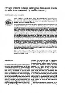
Figure 1 Growth Rates of Investment by Sectors in Humber Region GE Model Over 21st Century Growth Rate of Investment in Manufacturing Over Years
Growth Rate of Investment in Utilities Over Years
Growth Rate of Investment in Agriculture Over Years 1.8800
2.1600
1.8700
2.1400
1.8600
2.1200
1.7500 1.7000
1.8500 1.8400 1.8300
Growth rate
G rowth rate
2.1000 2.0800
1.6000 1.5500 1.5000 1.4500
2.0600 1.4000
1.8200 2.0400
2092
2087
2082
2077
2072
2067
2062
2057
2052
2047
2042
2037
2032
2027
2022
2017
2012
1997
2092
2087
2082
2077
2072
2067
2062
2057
2052
2047
2042
2037
2032
2027
2022
2017
2012
2007
1997
2092
2087
2082
2077
2072
2067
2062
2057
2052
2047
2042
2037
2032
2027
2022
2017
2012
2007
2002
1997
2002
2.0200
1.8000
2007
1.3500
1.8100
2002
Growth rate
1.6500
Years
Years
Ye ars
Growth Rate of Investment in Transport Over Years
Growth Rate of Investment in Distribution Over Years 1.8000
1.6000
1.6000
1.4000
1.4000
1.2000
1.2000
1.8450 1.8400
1.8100
0.6000
1.8050
0.4000
1.8000 2087
2092
2072
2077
2082
2077
2072
2067
2062
2057
2052
2047
2042
2037
2032
1997
Ye ars
2092
2087
2082
2077
2072
2067
2062
2057
2052
2047
2042
2037
2032
2027
2022
2017
2012
2007
Years
2002
1997
2092
2087
2082
2077
2072
2067
2062
2057
2052
2047
2042
2037
2032
2027
2022
2017
2012
2007
2002
1997
0.0000
2027
1.7950
0.2000
0.0000
1.8150
2022
0.2000
1.8200
2017
0.4000
0.8000
1.8250
2012
0.6000
1.0000
2007
0.8000
1.8300
2002
1.0000
1.8350 Growth rate
Growth rate
Growth rate
Growth Rate of Investment in Construction Over Years 1.8000
Ye ars
Growth Rate of Investment in Education and Public Services Over Years
Growth Rate of Investment in Business Finance Over Years
Growth Rate of Investment in Other Sector Over Years
1.8000
1.8950
1.9050
1.6000
Growth rate
1.8800 1.8750
1.9000
1.2000
1.8950
1.0000 0.8000 0.6000 0.4000
1.8700
1.8900 1.8850 1.8800
0.2000
1.8750
2092
2087
2082
2067
2062
2057
2052
2047
2042
2037
2032
2027
2022
2017
2012
2007
1.8700 2002
2092
2087
2082
2077
2072
2067
2062
2057
2052
2047
2037
2032
2027
2022
2017
2012
2042
Years
1997
2092
2087
2082
2077
2072
2067
2062
2057
2007
1997
Years
2052
2047
2042
2037
2032
2027
2022
2017
2012
2007
2002
1.8600
2002
0.0000
1.8650
1997
G rowth rate
1.8850
1.4000
Growth rate
1.8900
Years
45
Figure 2 Growth Rates of Capital Stock by Sectors in Humber Region GE Model Over 21st Century Growth Rate of Capital Stock in Agriculture Over Years
1.7500 1.7400 1.7300 1.7100 1.7000 1.6900
2.0600
1.6800
2.0400
1.6700 1.6600
2.0200
1.9800
Growth Rate of Capitla Stock in Distribution Over Years
1.7200
1.7500
1.7000
1.7000
2092
2087
2082
2077
2072
2067
2062
2057
1.8000 2092
2087
2082
2077
2072
2067
2062
2057
2052
1.7800 2092
2087
2082
2077
2072
2067
2062
2057
2052
2047
2042
2037
2032
1997
Ye ars
2027
1.7600
Ye ars
2022
2047
2042
2037
2032
2027
2022
2017
2012
2007
2002
1997
2092
2087
2082
2077
2072
2067
2062
2057
2052
2047
2042
2037
2032
2027
2022
2017
2012
1.8400 1.8200
1.4500
1.5600
1.8600
2017
1.5000
1.8800
2012
1.6000
2007
2052
1.9000
1.5500
2002
2047
1.9200
1.6000
1.6200
1.5800
1.9400
1.6500
2007
1.6400
1.9600
2002
1.6600
Growth Rate of Capital Stock in Transport Over Years
Growth rate
Growth rate
1.6800
1997
2042
2092
2087
2082
2077
2072
2067
2062
2057
2052
2047
2042
2037
2032
2027
2022
2017
2012
Years
Growth Rate of Capital Stock in Construction Over Years
Growth rate
2007
Years
2002
Years
1997
2092
2087
2082
2077
2072
2067
2062
2057
2052
2047
2042
2037
2032
2027
2022
2017
2012
2007
2002
1997
1.8200
2037
2.0000
2032
1.6500 1997
1.8300
1.7200
2027
1.8400
2.0800
2022
1.8500
2.1000
2017
Growth rate
1.8600
Growth rate
2.1200
2012
2.1400
2007
2.1600
1.8800
1.7600
2002
1.8900
1.8700 Growth rate
Growth Rate of Capital Stock in Manufacturing Over Years
Growth Rate of Capital Stock in Utilities Over Years
Years
Growth Rate of Capital Stock in Business Finance Over Years
Growth Rate of Capita Stock in Other Sector Over Years
Growth Rate of Capital Stock in Education and Public Services Over Years
2.0500
2.0000
1.8500
1.9500
1.8000
1.9000
1.7000
Years
46
2092
2087
2082
2077
2072
2067
2062
2057
2052
2047
2042
2037
2032
2027
2022
1997
2092
2087
2082
2077
2072
2067
2062
2057
2052
2047
2042
2037
2032
2027
2022
2017
2012
2007
2002
Years
1997
2092
2087
2082
2077
2072
2067
2062
2057
2052
2047
2042
2037
2032
2027
2022
2017
2012
1.5500
2017
1.6000
1.7000 2007
1.7500
1.6500
1.6000 2002
1.8000
1.7000
1.6500
1.7500
Years
1.8500
2012
1.8000
1.7500
2007
1.8500
G ro w th ra te
Growth rate
1.9000
1997
G rowth rate
1.9500
2002
2.0000
Figure 3 Growth Rates of Output by Sectors in Humber Region GE Model Over 21st Century Growth Rate of Agriculture Output Over Years
1.8800
2.1700
1.8600
2.1600
1.8400
1.7600
2.1100
1.7400
2.1000 2.0800
Ye ars
2092
2087
2082
2077
2072
2067
2062
2057
2052
2092
2087
2082
2077
2072
2067
2062
2057
2052
2047
Ye ars
2092
2087
2082
2077
2072
2067
2062
2057
2052
2047
2042
2037
2032
2027
2022
2017
2012
2007
1997
2.0700 2002
2042
2037
2032
2027
2022
2017
2012
2007
2002
1997
2.0900
2047
1.7200 1997
1.8200
1.7800
2042
1.8300
2.1200
1.8000
2037
1.8400
2.1300
2032
1.8500
1.8200
2027
1.8600
2022
Growth rate
2.1400
2017
1.8700
Growth rate
2.1500
2012
1.8800
2007
1.8900
2002
1.9000
Growth rate
Growth Rate of Manufacturing Output Over Years
Growth Rate of Utilities Output Over Years
Years
Growth Rate of Construction Output Over Years
Growth Rate of Transport Output Over Years
Growth Rate of Distribution Output Over Years 1.9650
1.8600
1.8800 1.9600
1.8400
1.8600 Growth rate
1.8400
1.8000
Growth rate
Growth rate
1.8200
1.7800 1.7600 1.7400
1.8200
1.9550 1.9500 1.9450
1.8000 1.9400
1.7800
1.7200
2092
2087
2082
2077
2072
2067
2062
2057
2052
2047
2042
2037
2032
2027
2022
2017
2012
2007
1997
2092
2087
2082
2077
2072
2067
2062
2057
2052
2047
2042
2037
2032
2027
2022
2017
2012
2007
2002
1997
Ye ars
Ye ars
Growth Rate of Business Finance Output Over Years
Growth Rate of Other Sector Output Over Years
Growth Rate of Education and Public Services Output Over Years
2.0600
1.9000
2.0550
1.8900
2.0500
2.0300 2.0250
1.8800
2.0050
2092
2087
2082
2077
2072
2067
2062
2057
2052
2047
2042
2037
2032
2027
2022
2017
2092
2087
2082
2077
2072
2067
2062
2057
2052
2047
2042
2037
2032
2012
2.0000
1.8100 2027
2092
2087
2082
2077
2072
2067
2062
2057
2052
2047
2037
2032
2027
2022
2017
2012
2007
2002
1997
2042
Ye ars
2.0100
2007
1.8200
2.0150
2002
2.0100
2.0200
1997
1.8300
2.0050
Growth rate
1.8400
2.0150
2022
2.0200
1.8500
2017
2.0250
2012
2.0300
1.8600
2007
2.0350
1.8700
2002
Growth rate
2.0400
1997
2.0450 Growth rate
Years
1.7400
2092
2087
2082
2077
2072
2067
2062
2057
2052
2047
2042
2037
2032
2027
2022
2017
2012
2007
2002
1997
1.6800
2002
1.9350
1.7600
1.7000
Ye ars
Ye ars
47
Conclusions of this study •
First input output table for Humber Region: Hull, East Riding, North Lincolnshire and North East Lincolnshire
•
First regional multisectoral general equilibrium model for Humber regions.
•
First dynamic model for Hull
•
Regional comparison is made for output, employment, capital and aggregate supply – dynamic growth paths are evaluated based on current preferences and technology for coming hundred years
•
Useful for policy analysis.
•
Programmes and worksheets containing model are available. 48
References Becker, R. A. (1980) On The Long-Run Steady State In A Simple Dynamic Model Of Equilibrium With Heterogeneous Households Quarterly Journal Of Economics September, pp.375-382. Bhattarai, K. (2007) Input-Output and General Equilibrium Models of Hull and Huumber Region in England, forthcoming in Atlantic Economic Journal. Bhattarai, K.(2005) Welfare Impacts of Equal-Yield Tax Experiment in the UK Economy, Applied Economics, forthcoming. Bhattarai, K and Whalley J.(2000) General Equilibrium Modelling of UK Tax Policy in S. Holly and M Weale (eds.) Econometric Modelling: Techniques and Applications, pp. 69-93, the Cambridge University Press. Bhattarai, K and Whalley, J.(2006) Division and Size of Gains from Liberalization of Trade in Services, Review of International Economics, 14:3:348-361. Central Unit for Environmental Planning. (1969) Humberside : A Feasibility Study, the Central Units of Environmental Planning, London : H.M.S.O., 1969. Chamley, C. (1985) Efficient Tax Reform In A Dynamic Model Of General Equilibrium The Quarterly Journal Of Economics ,May, pp:336-356. Dietzenbacher, E. and Stage, J. (2006) Mixing Oil and Water? Using Huybrid Input_Output Tables in a Structural Decomposition Analysis, Economic Systems Research, 18:1:85-95. Elbers, C. (1992) Spatial Disaggregation in General Equilibrium Models: With an Application to the Nepalese Economy, Free University Press, Amsterdam. Hull. City and County Council. (1970s) Development Opportunities in Kingston upon Hull, the Directorate of Industrial Development Hull. Humber Forum (2003) Bridging the Gap: the Strategic Framework for Economic Development in the Humber and Hull Advanced Economy policy documents, www.humberforum.com, August. Jackson, R. W. (1998) Regionalizing National Commodity-by-Industry Accounts ; Economic Systems Research, September v. 10, iss. 3, pp. 223-38 Judd, K.L., Kubler, F. and Schmedders, K.(2000) Computing Equilibria In Infinite-Horizon Finance Economies: The Case Of One Asset, Journal Of Economic Dynamics & Control 24 ,1047-1078
49
References Kehoe, T. J. (1985)The Comparative Static Properties of Tax Models, Canadian Journal of Economics, May, v. 18, iss. 2, pp. 314-34 King, M. A. and Robson, M. H. (1993) A Dynamic Model of Investment and Endogenous Growth, Scandenevian Journal of Economics, 95(4) 445-446. Pyatt, G. (1963) A Measure of Capital, The Review of Economic Studies, 30: 3: 195-202 Pyatt, G and Round, J.I.(1979) Accounting and Fixed Price Multipliers in a Social Accounting Matrix Framework, The Economic Journal , 89 :356: pp. 850-873 Rutherford, T. F. (1998) GAMS/MPSGE Guide: GAMS Development Corporation, Washington DC. Leontief, W. (1949) Structural Matrices of National Economy, Econometrica, 17: 273-282, Suppl. Leahy, K. and Williams, D. (1996) North Lincolnshire : a pictorial history Cherry Burton : Hutton Press. Manners, G., Keeble D. Rodgers, B. and Warren, K. (1972) Regional Development in Britain, John Wiley and Sons, London. Miller, M.H. and Spencer, J.E. (1977) The Static Economic Effects of the UK Joining the EEC: A General Equilibrium Approach , The Review of Economic Studies, Vol. 44, No. 1 Feb., pp. 71-93 Macmahon, K. A. (1961) Acts of Parliament and proclamations relating to the East Riding of Yorkshire and Kingston upon Hull, 1529-1800 Hull : University Office for National Statistics (ONS (1995)) Input Output: Tables for the United Kingdom, HMSO, London. Robinson, S. (1991) Macroeconomics, Financial Variables, and Computable General Equilibrium Models, World Development, vol. 19, no.11, pp.1509-1523, Pergamon Press plc. Scarf, H. E. (1986) The Computation of Equilibrium Prices, in Scarf, H. E and Shoven, J. B. ed. Applied General Equilibrium Analysis, Cambridge University Press. Shoven, J. B. and Whalley, J. (1992) Applying General Equilibrium, Cambridge University Press.. Whalley J. (1985) Trade Liberalization Among Major World Trading Areas, MITPress, Cambridge. Wood, D.M. (1988) Will the North rise again? Local Economic Regeneration in Yorkshire/Humberside and North East England, Hull Papers in Politics no. 41. Hull University Politics Department. Heng-Fu, Z. (1996) Taxes, federal grants, local public spending, and growth Journal of Urban Economics 39, 303-317 article no. 0016.
50
51
http://www.hull.ac.uk/wise/
52


![AC2[R+,R] - Hindawi](https://m.moam.info/img/260x300/ac2rr-hindawi_5b5b550f097c47ff718b4589.jpg)

!['[--)][' R·-E···' CT()R](https://m.moam.info/img/260x300/-r-e-ctr_5a2f16371723dddcaca8f531.jpg)


