Real-Time Compression for Dynamic 3D Environments Sang-Uok Kum
[email protected]
Ketan Mayer-Patel
[email protected]
Henry Fuchs
[email protected]
University of North Carolina at Chapel Hill CB#3175, Sitterson Hall Chapel Hill, NC 27599 USA
The goal of tele-immersion has long been to enable people at remote locations to share a sense of presence. A tele-immersion system acquires the 3D representation of a collaborator’s environment remotely and sends it over the network where it is rendered in the user’s environment. Acquisition, reconstruction, transmission, and rendering all have to be done in real-time to create a sense of presence. With added commodity hardware resources, parallelism can increase the acquisition volume and reconstruction data quality while maintaining real-time performance. However this is not as easy for rendering since all of the data need to be combined into a single display. In this paper we present an algorithm to compress data from such 3D environments in real-time to solve this imbalance. We expect the compression algorithm to scale comparably to the acquisition and reconstruction, reduce network transmission bandwidth, and reduce the rendering requirement for real-time performance. We have tested the algorithm using a synthetic office data set and have achieved a 5 to 1 compression for 22 depth streams.
Network and Services, Inc. [1] have been actively developing tele-immersion systems for several years. There are three main components to a tele-immersion system: scene acquisition, 3D reconstruction, and rendering. Figure 1 shows a block diagram relating these components to each other and the overall system. The scene acquisition component is comprised of multiple digital cameras and PCs. The digital cameras are placed around the scene to be reconstructed. The cameras are calibrated and registered to a single coordinate system called the world coordinate system. PCs are used to synchronize the cameras and control image transfer to the 3D reconstruction system. The 3D reconstruction system uses the captured images from the acquisition system to create real-time depth streams [9]. A depth stream is a video stream augmented with per-pixel depth information from the world coordinate system. Three input images are used to create one depth stream. The images are rectified and searched for correspondences between images. Using the correspondence information, disparities at each pixel are computed. The computed disparities and the calibration matrices
Categories and Subject Descriptors I.3.2 [Computer Graphics]: Graphics Systems – distributed/network graphics. I.3.7 [Computer Graphics]: ThreeDimensional Graphics and Realism – virtual reality. I.3.7 [Computer Graphics]: Applications. H.3.3 [Information Storage and Retrieval]: Information Search and Retrieval Clustering.
Keywords Real-Time Compression, Tele-Immersion, Virtual Reality, KMeans algorithm, K-Means initialization.
3D Camera 2D Camera
Remote Scene
2D Camera 2D Camera 2D Camera
1. INTRODUCTION Tele-immersion creates a sense of presence with distant individuals and situations by providing an interactive 3D rendering of remote environments. The 3D Tele-Immersion research group at the University of North Carolina, Chapel Hill [10] together with collaborators at the University of Pennsylvania [17], the Pittsburgh Supercomputing Center [11], and Advanced
Permission to make digital or hard copies of all or part of this work for personal or classroom use is granted without fee provided that copies are not made or distributed for profit or commercial advantage and that copies bear this notice and the full citation on the first page. To copy otherwise, or republish, to post on servers or to redistribute to lists, requires prior specific permission and/or a fee. MM’03, November 2-8, 2003, Berkeley, California, USA. Copyright 2003 ACM 1-58113-722-2/03/0011…$5.00.
3D Reconstruction
2D Camera 2DCamera Camera 3D 3D Camera 3D Camera 3D Camera 3D Reconstruction
Rendering System user location Remote Scene
Display Screen
ABSTRACT
User
Figure 1. Tele-Immersion System: The 2D cameras acquire images of the scene and transmit them to the 3D reconstruction where depth streams are created. The depth streams are sent to the rendering system for view-dependent rendering of the scene.
of the cameras are used to compute the world coordinates of each 3D point. The acquisition and 3D reconstruction systems can be thought of as an array of 3D cameras (i.e., a camera that creates a depth stream with color and depth information at each pixel). Each 3D camera is associated with a specific viewpoint and view direction defined in the world coordinate system. The depth streams are sent to the rendering system to be rendered and displayed in head-tracked passive stereo [3]. Since the depth streams are in world coordinates, thus view-independent, they can be rendered from any new viewpoint. The user’s head is tracked to render the depth streams from precisely the user’s current viewpoint to provide a sense of presence. For effective, interactive operation, a tele-immersion system must accomplish all of these tasks in real-time. A number of system resources must be carefully managed including: Network bandwidth. The acquired images must be sent to the 3D reconstruction system and the resulting depth streams sent to the rendering system. Even at a modest frame rate of 10 fps and an image resolution of 640x480 with 8 bits per pixel, 24.5 Mbs per 2D camera is required. Compressing the image streams is generally not possible due to severe artifacts created by most coding techniques during the 3D reconstruction process. The reconstructed depth streams must also be transmitted to the remote rendering system. At 640x480 resolution, each depth stream is 12.3Mbits per frame (i.e., 3 bytes for color and 2 bytes for depth). Without data compression, 10 depth streams at 10 fps would produce data at 1.23 Gbps to the rendering system. Computation. The correspondence between images must be calculated in order to create depth streams in the world coordinate system. Fortunately, this process can be parallelized to achieve real-time performance as each depth stream computation is independent of the others. Rendering. At a resolution of 640x480, each frame of each depth stream is comprised of approximately 300K 3D points. A system with ten depth streams would require 90 Mpts/sec rendering performance to achieve 30 fps view-dependent rendering which is difficult with currently available commodity hardware. Rendering is not as easily parallelized as 3D reconstruction since all of the depth streams must be rendered into a single view. Our initial prototype system used fifteen cameras and five quadprocessor PCs for image acquisition and 3D reconstruction. Each PC was connected to three cameras for image acquisition. These five PCs were also used for 3D reconstruction, creating one depth stream per PC using the three cameras as input. The five reconstructed depth streams were sent over Internet-2 to a remote rendering system, which were interactively rendered in stereo using three additional PCs [16]. A major bottleneck of this system was the computational demand of the 3D scene reconstruction. The system was only able to use 320x240 resolution images and only processed the foreground. The resulting acquisition volume was only approximately one cubic meter and the reconstruction rate was limited to 1-2 fps. The rendering system combined the 320x240 resolution depth streams with a previously modeled 3D office as a background and displayed the result in head-tracked stereo at 40-50 fps.
The next system improved the volume of the acquisition space and resolution of the streams [6]. Scene acquisition was performed using 27 cameras and 9 PCs – each PC connected to 3 cameras. These cameras were capable of capturing 640x480 resolution images at 30 fps. These images were sent uncompressed to the Terascale Computing System at the Pittsburgh Supercomputing Center using Gigabit Ethernet and Internet-2 for 3D scene reconstruction. Nine depth streams at 640x480 resolution with no background subtraction were computed at 8 fps by the reconstruction system. The depth streams were sent to a 3 PC rendering system also using Internet-2 and Gigabit Ethernet. However due to the limits of the rendering system, the system was only able to achieve 1-2 fps end-to-end. While the scene acquisition and 3D reconstruction processes can be parallelized by adding additional hardware resources, experience with our initial prototypes indicate that rendering performance is likely to remain a bottleneck. One way to alleviate this bottleneck is to exploit coherence between the reconstructed depth streams and remove redundant points. Doing so reduces the number of points that are communicated to the rendering system while maintaining the quality of the reconstruction. In this paper, we present techniques for exploiting coherence between depth streams in order to find and eliminate redundant points. Our contributions include: • A real-time depth stream compression technique. Our Group Based Real-Time Compression finds and eliminates redundant points between two or more depth streams. • A depth stream coherence metric. In order to efficiently employ Group Based Real-Time Compression, we must be able to compute which depth streams are most likely to exhibit strong coherence. We present an efficient algorithm for partitioning depth streams into coherent groups. This paper is organized as follows. Section 2 describes background and related work. Section 3 provides an overview of our approach and a comparison with other possible approaches. In Section 4 we present the compression algorithm in detail. Section 5 explains how streams are partitioned into coherent groups. We give performance results in Section 6, and present our conclusions and future work in Section 7.
2. BACKGROUND AND RELATED WORK We are not aware of any work on real-time compression of dynamic 3D environments. There is, however, related work on compressing static environments. McMillan and Bishop [7] proposed using a depth image (i.e., an image with color and depth information) to render a scene from new viewpoints by warping the depth image. One of the major problems is disocclusion artifacts caused when a portion of the scene not visible in the depth image is visible from the new viewpoint. Using multiple depth images from multiple viewpoints can reduce these disocclusion artifacts. Layered Depth Images (LDI) merge multiple depth images into a single depth image by keeping multiple depth values per pixel [14]. However, the fixed resolution of an LDI imposes limits on sampling multiple depth images. LDI tree, an octreee with a single LDI in each node, can be used to overcome this limitation [2]. Grossman and Dally [4] create multiple depth images to model an arbitrary synthetic object. The depth images are divided into 8x8 blocks and redundant blocks are removed. QSplat [13] uses a
bounding sphere hierarchy to group 3D scanned points for realtime progressive rendering of large models. All of the previous research described above dealt with static data in which compression was done only once as a preprocessing step. These techniques are not suitable for real-time dynamic environments in which the compression has to be done every frame. There has been special scalable hardware developed to composite images with depth information [8, 15]. The rendering system can be parallelized using these special hardware by connecting each 3D camera to a rendering PC and then compositing all of the rendered images. Unfortunately these systems are not commonly available and expensive to build.
3. OVERVIEW AND DESIGN GOALS This section outlines our design goals for the compression algorithm, examines several possible approaches to the problem and gives an overview of our Group Based Real-Time Compression.
3.1 Design Goals In order to ensure a high quality rendering, we will require that the depth stream that most closely matches the user’s viewpoint at any given time is not compressed. We will call this depth stream the main stream. All points of the main stream are transmitted to the rendering process. Furthermore, a subset of the depth streams is identified as the set of reference streams. The reference streams form a predictive base for detecting and eliminating redundant points and are distributed among the reconstruction processes. Every stream except for the main stream is compared to one or more of the reference streams and redundant points are eliminated. The result is called a differential stream. These differential streams and the main stream are sent to the rendering system. Our design goals for the compression algorithm include: • Real-time performance. The compression algorithm needs to be at least as fast as the 3D reconstruction so there is no delay in processing the streams. • Scalability. The algorithm needs to scale with the number of 3D cameras, so that as the number of 3D cameras increases the number of data points does not overwhelm the rendering system. • Data reduction. In order to alleviate the rendering bottleneck, the algorithm needs to reduce the number of data points by eliminating as many redundant points as possible. • Tunable network bandwidth. Distributing reference streams to the reconstruction processes will require additional network bandwidth. The algorithm should be tunable to limit the network bandwidth used even as the total number of depth streams increases.
3.2 General Approaches Given the restrictions and design goals outlined above, there are a number of general approaches that may be incorporated into our solution.
3.2.1 Stream Independent Temporal Compression One possible approach is to compress each stream independently using temporal coherence. With such an approach, each stream acts as its own reference stream. Exploiting temporal coherence for traditional video types is known to result in good compression for real-time applications. This compression scheme scales well, and requires no additional network bandwidth since there is no need to communicate reference streams among the reconstruction processes. However this compression scheme does not reduce any data points that the renderer must render each frame. The renderer must render all redundant points from the previous frame with the non-redundant points of the current frame.
3.2.2 Best Interstream Compression The best possible interstream compression would be to remove all redundant points from all streams by using every stream as a possible reference stream. This could be accomplished in the following way. The first stream sends all of its data points to the rendering system and to all other reconstruction processes as a reference stream. The second stream uses the first stream as a reference stream, creating a differential stream which it also distributes to the other reconstruction processes as a reference stream. The third stream receives the first two streams as reference streams in order to create its differential stream, and so on, continuing until the last stream uses all other streams as reference streams (Figure 2a). This is the best possible interstream compression since it has no redundant points. The drawbacks to this approach, however, are severe. Most streams in this approach require multiple reference streams with at least one stream using all other streams as references. This dramatically increases computation requirements and makes realizing a real-time implementation very difficult. Also the number of reference streams broadcast is dependent on the number of streams. Thus the network bandwidth required will increase as the number of streams increases, limiting scalability of the 3D cameras.
3.2.3 Single Reference Stream Compression Another approach is to use the main stream as the reference stream for all other streams (Figure 2b). This does not require additional network bandwidth as more streams are added since there is always one reference stream. Real-time operation is feasible since all other streams are compared against only one reference stream. A main disadvantage of this approach is possibly poor data compression. The coherence between the main stream and the depth streams that use it as a reference stream is 1
1
2
3 (a)
4
2
3
4
5
(b)
5 1
2
3 (c)
4
5 (b)
Figure 2. Examples of different compression algorithms and its reference stream transfer. The main stream is in bold and the arrows show the direction of reference stream movement. (a)Best Interstream Compression. (b)Single Reference Stream Compression. (c)Neighbors as Reference Stream Compression.
likely to diminish as the viewpoints of the streams diverges. Furthermore, the depth streams from two nearby viewpoints may contain redundant points which are not removed by using the main stream as the only reference.
Stream 4
Stream 5
Stream 6
Stream 1
Stream 2
Stream 3
Stream 7
Stream 8
Stream 9
3.2.4 Neighbors as Reference Stream Compression Another approach is for each depth stream to select the closest neighboring depth stream as the reference stream to achieve better compression. The streams can be linearly sorted such that neighboring streams in the list have viewpoints that are close to each other. From this sorted list of streams, the streams left of the main stream use the right neighboring stream as its reference stream, and the streams right of the main stream uses the left neighboring stream as its reference stream (Figure 2c). With this scheme, every stream has one reference stream regardless of the total number of streams. The compression rate depends on the number of points that appear in non-neighboring streams but not in neighboring streams since these points will be redundant in the final result. Since the streams are sorted, the number of redundant points in non-neighboring streams but not in neighboring streams should be small which makes the compression comparable to the previously mentioned Best Interstream Compression method. However the network bandwidth demand for this compression scheme is high. For n streams there are n-1 reference streams to distribute, again limiting scalability of 3D cameras.
3.3 Overview of Our Approach Group Based Real-Time Compression tries to balance compression efficiency and network bandwidth requirements by limiting the number of reference streams to a configurable limit and grouping streams together based on which of these streams serves as the best reference stream to use. All streams are divided into groups such that each stream is part of only one group. Each group has a center stream that is a representative of the group and sub streams (i.e., all other streams in the group). Stream partitioning and center stream selection is done as a preprocessing step. The main stream and the center streams are possible reference streams. Thus the number of reference streams distributed equals the number of groups created plus one – the main stream. Each stream selects the reference stream that will generate the best compression and creates a differential stream. Since the number of reference streams is limited to the number of groups, new streams can be added without increasing the reference stream network traffic. Also each stream only uses one reference stream to create its differential frame, which makes realtime operation feasible. The compression algorithm is described in more detail in Section 4. Section 5 details how streams are partitioned into groups and the center stream for each group selected.
4. STREAM COMPRESSION This section details how depth streams are compressed in realtime. First we detail how reference streams are selected for each stream, and then discuss how these streams are compressed using the selected reference stream.
4.1 Reference Stream Selection In Group Based Real-Time Compression, all depth streams are partitioned into disjoint groups. The number of groups created is determined by the network bandwidth. Each group has a center
Group 2
Group 1
Group 3
Figure 3. An example of reference stream transfer for Group Based Real-Time Compression. Stream 2 is the main stream, which makes Group 1 the main group. Streams 1,4, and 7 are the center streams for its group. The arrows show the direction of the reference stream movement. stream, which best represents the group, and sub streams – depth streams in a group that are not the center stream. Furthermore, one stream is selected as the main stream for which no compression is done. The depth stream viewpoint with the shortest Euclidian distance to the user is chosen as the main stream since it best represents the user’s viewpoint. The group containing the main stream is called the main group and all other groups are referred to as a sub group. Once the main stream has been selected, the reference stream for all streams are selected as follows: • For the main stream, no reference stream is needed. • For the center stream of the main group, the main stream is used as the reference stream. • For the center streams of the sub groups, the center stream of the main group is used as the reference stream. • For any other substream, the center stream of its group is used as the reference stream. An example is shown in Figure 3.
4.2 Differential Stream Construction To construct a differential stream, the data points of a depth stream are compared to the data points within the reference stream. Points that are within some given distance threshold are removed from the depth stream. The format of the differential stream is different from the original stream format. The original stream has five bytes, three bytes for color and two bytes for depth, for each data point. The differential stream has five bytes for only the non-redundant points (i.e., points not removed) and a bitmask to indicate which points have been retained and which points have been eliminated. If the bit value is ‘0’ then the data point represented by the bit is a redundant point and is removed. If the bit value is ‘1’, the corresponding point is included. The order of data for nonredundant points is the same as the order it appears in the bitmask. This format reduces the size of a frame in the differential stream by 39 bits, five bytes minus one bit, for redundant points and adds 1 bit for non-redundant points. So for a depth stream of 640x480 resolution with a 5 to 1 redundancy ratio (i.e., 80% of data points
Redundant Points (%)
where stream Si and Sj is in group k, and nk is the number of streams in group k
100
The group squared angle sum(GSAS), defined for a given group, is the sum of the squared angle between the group’s center stream and every sub stream in the group (equation (2)). This is used as the partitioning criterion for partitioning n streams into k groups. The sum of all GSAS’s for a particular partition (equation (3)) is defined as the total squared angle sum (TSAS). We are seeking the partition that minimizes TSAS.
80 60 40 20
nj
0 0
20
40
60
80
Angle Between Two Streams (degree) Figure 4. Percentage of redundant points of a stream in the reference stream vs. the angle between the two streams. The percentage of redundant points decrease as the angle increases. The streams are from the 3D camera configurations of Figure 9. are deemed redundant), the data will be reduced from 1.536MB to 346KB – approximately 5 to 1.
5. STREAM PARTITION As discussed above the streams need to be partitioned into groups. In this section we present an effective criterion to partition n streams into k groups and to find the appropriate center stream in each group. We further use the criteria to develop an efficient approximate algorithm for stream partitioning and center stream selection when n is too large for an exhaustive approach.
5.1 Coherence Metrics Stream partitioning and selection of center streams has a direct impact on compression since all sub streams of a group use the center stream of the group as the reference stream. Therefore the partitioning should ensure that each stream belongs to a group where the volume overlap between the stream and the group center stream is maximized. However, exact calculation of the volume overlap between two streams is expensive. Thus, in this paper we propose using the angle between the view directions of two depth streams as an approximation of the overlapped volume. Characteristically, teleimmersion applications generally organize depth streams to point toward a common area (i.e., the acquisition volume). Also the volumes of the depth streams are symmetric, making the angle between the view directions of two streams a good estimate for how much the two stream volumes overlap. The smaller the angle, the bigger the overlap. This is shown in Figure 4. The local squared angle sum (LSAS) is defined for stream Si as the sum of the squared angle between stream Si and all other streams in its group (equation (1)). This is used as the center stream selection criterion. The stream with the lowest LSAS of the group is chosen to be the center stream. nk LSASi = ∑ [angle of (Si, Sj)] 2, j=1
(1)
GSASi = ∑ [angle of (Cj, Sji)] 2, (2) i=1 where Cj is the center stream in group j, Sji is a sub stream in group j, and nj is the number of streams in group j k TSAS = ∑ GSASi, i=1 where k is the number of groups
(3)
Finally, the central squared angle sum (CSAS) is defined as the sum of the squared angle between all center streams (equation (4)). The streams should be partitioned such that CSAS is also minimal, since all center streams use each other as references. However, it should be noted that minimizing TSAS is much more important than minimizing CSAS since TSAS effects compression much more than CSAS. k-1
CSAS = ∑
k
∑
[angle of (Ci, Cj)] 2,
i=1 j=i+1
(4)
where Ci and Cj is and center stream for group i and j, and k is the number of groups
5.2 Exhaustive Partition One way to partition n streams into k groups is an exhaustive method where all possible grouping combinations are tested. First k streams are selected from n streams. The selected streams are chosen as center streams and all other streams are assigned to the group with which the absolute angle of the stream and the group’s center stream is the smallest. This is done for all possible combinations of selecting k streams from n streams – a total of nCk. For each stream partitioning the TSAS is calculated and the stream partitioning with the lowest TSAS is the partitioning solution. If there are multiple stream partitions with the same TSAS, the stream partition with the lowest CSAS is chosen as the solution. Unless n is small, this method is not practical.
5.3 Approximate Partition The k-means framework [5], original developed as a clustering algorithm, can be used to partition the streams for an approximate solution. The k-means framework is used to partition n data points into k disjoint subsets such that a criterion is optimized. The kmeans framework is a robust and fast iterative method that finds the locally optimal solutions for the given criteria. It is done in the following three steps. • Initialization: Initial centers for the k partitions are chosen. • Assignment: All data points are placed in the partition with the center that best satisfies the given criteria. Usually the
criteria are given as a relationship between a data point and the center.
S1
S2
S3
• Centering: For each partition the cluster centers are reassigned to optimize the criteria. The assignment and centering steps are repeated until the cluster centers do not change or an error threshold is reached.
5.3.1 Iterative Solution for Approximate Partitioning Given initial center streams, the criteria used to assign all sub streams to a group is the absolute angle of the stream and the group’s center stream. The sub streams are assigned such that this absolute angle is the smallest. This would give groupings where the TSAS is minimized. After every sub stream has been assigned to a group, each group recalculates its center stream where the stream with the lowest LSAS is the new center stream of the group. The process of grouping and finding the center stream is repeated until the center streams converge and does not change between iterations.
5.3.2 Center Stream Initialization The performance of this approximate approach heavily depends on the initial starting conditions (initial center streams and stream order) [12]. Therefore in practice, to obtain a near optimal solution, multiple trials are attempted with several different instances of initial center streams. The full search space for the iterative method could be investigated when all possible starting conditions – total of nCk – are explored. A starting condition is given as a set of k initial center streams. As seen in Table 2, such an exhaustive method will find all possible ending conditions. For example, if n=10 and k=5, then there would be a total of 10C5 = 252 possible starting conditions, which in the example in Table 2 will lead to one of 46 distinct ending conditions. An ending condition is one in which the center streams do not change from one iteration to the next. The optimal answer is obtained by examining TSAS of all ending conditions. If there are multiple ending conditions with the same TSAS, the CSAS is used. However for numbers of n and k where this becomes impractical, we can examine only a small sample of all the possible starting conditions. The chances of finding the same optimal solution as the exhaustive method will increase by intelligently selecting the starting conditions to examine. Theoretically, the best way to initialize the starting center streams is to have the initial center streams as close to the optimal answer as possible. This means that in general the initial centers should be dispersed throughout the data space. In this section, we discuss a method for finding starting center stream assignments that are well-dispersed in the data space. Once good starting conditions have been identified, it is straightforward to examine all corresponding ending conditions to find a near-optimal solution. The basic approach to identifying all possible good starting conditions is as follows: (1) Sort the given streams using global squared angle sum. (2) Group the streams in all possible “reasonable” ways. (3) Find all possible “reasonable” candidate center streams. (4) Generate all possible combination of the candidate center streams for each possible grouping as good starting conditions.
Figure 5. Dominant Stream: Streams S1, S2, and S3 all have zero angle with each other. Stream S1 covers stream S2 and S3 since any data point in S2 and S3 is also in S1. Therefore S1 is the dominant stream. The arrow indicates the stream view direction. (5) Remove all duplicates.
5.3.2.1 Stream Sorting Although the streams cannot be strictly ordered due to the threedimensional nature of the viewpoint locations, an approximate sorting using the global squared angle sum is sufficient for our purpose. Global squared angle sum (GlSAS) for stream Si is the sum of the squared angle between steam Si and all other given streams (equation (5)). n GlSASi = ∑ [angle of (Si, Sj)] 2, (5) j=1 where Si and Sj are streams, and n is the total number of streams Given total of n streams, the pivot stream is chosen as the stream with the lowest GlSAS. Next all other streams are divided into three groups – streams with a negative angle with respect to the center stream, streams with a positive angle, and streams with zero angle. Any stream that has zero angle with the center stream, either covers the pivot stream or is covered by the pivot stream. All such streams except for the dominant stream (i.e., the stream that covers all other streams) are removed from the stream list. Figure 5 illustrates the notion of a dominant stream. These removed streams are added back as sub streams to the dominant stream’s group after the near-optimal solution has been found. The positive angle and negative angle groups are each sorted using the GlSAS. The negative angle streams are sorted in descending order and the positive angle streams are sorted in ascending order. Placing the sorted negative angle streams left and the sorted positive angle streams on the right of the pivot stream creates the final sorted list.
5.3.2.2 Initial Group Partitions After the n streams are sorted, they are partitioned into k initial groups. To ensure that we include all possible good starting conditions, we consider all reasonable groupings. Next we describe our heuristics for creating reasonable groupings. The k initial groups are created such that, • If stream Si is in group Gj, stream Si+1 is either in group Gj or Gj+1 where 1 ≤i≤n, 1≤j≤k, and stream Si is left of stream Si+1 in the sorted stream list. • If n is not an exact multiple of k, every group is assigned either n/k or n/k streams and every stream is assigned to a group. If n is an exact multiple of k one group is assigned (n/k)-1 streams, another is assigned (n/k)+1 streams, and every other group is assigned n/k streams.
1 2 3 | 4 5 6 | 7 8 9 10 1 2 3 | 4 5 6 7 | 8 9 10 1 2 3 4 | 5 6 7 | 8 9 10 (a)
12|345|6789 12|3456|789 123|45|6789 123|4567|89 1234|567|89 1234|56|789
123|456|789 (b)
(c)
Figure 6. Initial Group Partitions: (a)All possible initial group partitions for 10 streams into 3 groups. (b)Only one grouping is possible for 9 streams and 3 groups with normal conditions. (c)All possible initial group partitions for 9 streams into 3 groups. Streams are grouped into every possible combination that meets the above reasonableness criteria. Figure 6a shows the three possible groupings of 10 sorted streams into 3 groups. The special case when n is an exact multiple of k is treated differently because the normal conditions will only allow one possible partition (Figure 6b). In order to generate multiple partitions, one group is assigned (n/k)-1 streams and another is assigned (n/k)+1 streams, and every other group is assigned n/k streams (Figure 6c).
5.3.2.3 Candidate Centers Again to ensure all possible good starting conditions are included, multiple center stream candidates are chosen for each group. If the group has even number of streams, the two streams in the middle are chosen as candidates. If it has odd number of streams, the middle stream and its two neighboring streams are chosen as candidates (Figure 7a).
(a)
(a) 1 2 3 | 4 5 6 | 7 8 9 10 {1, 4, 8}, {1, 4, 9}, {1, 5, 8}, {1, 5, 9}, {1, 6, 8}, {1, 6, 9}, (b) {2, 4, 8}, {2, 4, 9}, {2, 5, 8}, {2, 5, 9}, {2, 6, 8}, {2, 6, 9}, {3, 4, 8}, {3, 4, 9}, {3, 5, 8}, {3, 5, 9}, {3, 6, 8}, {3, 6, 9} Figure 7. Initial Center Streams: (a)10 streams partitioned into 3 groups. The candidate centers are in bold. (b)Initial center streams generated from group partition (a). Total of 18 initial center streams have been generated for this instance.
5.3.2.4 Generating Initial Starting Points Finally we select a set of k center streams, one from each group, to construct a starting condition. All possible combinations for the candidate centers are generated as good beginning conditions (Figure 7b). Note that when all possible starting conditions for all possible combinations are generated there will be duplicate starting conditions, and these are removed. The distinct starting conditions generated will be the good starting conditions explored. If the number of starting conditions is still too large, the desired number of initial sets can be stochastically sampled from all identified good starting conditions. In this case, the duplicates are not removed when sampling in order to provide those conditions with a better chance of being sampled.
6. RESULTS In this section we present our results for depth stream compression and depth stream partitioning. Stream compression was tested on two different camera configurations similar to the ones used in previous systems [6, 16]. The stream partition algorithm was tested on randomly placed cameras as well as the configuration used to test stream compression.
(b)
Figure 8. (a)Synthetic Office Layout (b)Rendered Images of the Synthetic office.
1
3
2
4 5
6
7
8 9 10
11
12
13
12
13
14
15
16
17
18
19
20
21
22
1
2
3
4
5
6
7
8
9
10
11
(b) 5 (b) Figure 9. 3D Camera Configuration: The 3D cameras are partitioned using the algorithm given in the paper. The 3D cameras in circled numbers are the center camera of the group. (a)Top view of 13 3D camera configuration partitioned into 3 groups. The 3D cameras are placed 2m from the mannequin in a semicircle at mannequin’s eye height. The distance between neighboring cameras is 20cm. (b)Frontal view of 22 3D cameras configuration partitioned into 5 groups. The 3D cameras are placed on a wall 2.25m from the mannequin. The vertical and horizontal distance between 3D cameras is 20cm. The bottom row is at mannequin’s eye height.
Table Mannequin (a)
6.1 Stream Compression
6.1.1 Compression Speed The average compression speed for the both 3D camera configurations was 0.099sec/frame. The minimum time was 0.080sec/frame for the both configurations. The maximum time was 0.104sec/frame for the first configuration of 13 3D cameras and 0.107sec/frame for the second 22 3D camera configuration. These results show that the compression algorithm is able to handle 10 frames/sec on the average and 9.3 frames/sec in the worst case. This is fast enough to handle the 3D reconstruction of 8 frames/sec given in [6]. All of the results were obtained using a PentiumIV 2.4GHz machines with 1GB of memory running Linux.
6.1.2 Compression Rate Figure 10 shows a comparison of compression rates for Group Based Real-Time Compression, Best Interstream Compression and Neighbors as Reference Stream Compression. The Best Interstream Compression was chosen since it is the best compression achievable, and the Neighbors as Reference Stream
12
7 6 5 4 3 2 1 0
10 8 Best
6
Neighbor
4 2
Real-Time
Compression Rate
Compression Rate
We tested the Group Based Real-Time Compression algorithm on two different 3D camera configurations of a synthetic office [3]. Figure 8a shows the layout of the synthetic office and Figure 8b is an image of the rendered office. The first configuration placed 13 3D cameras around the scene in a semi-circle. The 3D cameras were placed about 2m from the mannequin at its eye height and was pointed at the mannequin’s head. The 3D cameras were placed about 20cm apart [16] (Figure 9a). The second configuration placed 2 rows of 11 3D cameras on a wall 2.25m from the mannequin. The two rows were parallel and 20cm apart with the bottom row at the height of the mannequin’s eye. Cameras in each row were placed at 20cm intervals and pointed at the mannequin’s head [6] (Figure 9b). The depth stream from each 3D camera was at a resolution of 640x480 without any background subtraction. The horizontal field of view for all of the cameras was 42 degrees.
0 0
2
4
6 8 Main Stream (a)
10
12
0
2
4
6
8 10 12 14 16 18 20 22 Main Stream (b)
Figure 10. Compression rates of different schemes. ‘Best’ shows Best Interstream Compression, ‘Neighbor’ the Neighbors as Reference Stream Compression, and ‘Real-Time’ the Group Based Real-Time Compression. (a)13 streams from Figure 9a (b)22 streams from Figure 9b
PSNR Neighbor Real-Time
Camera Config
Vie w
Main Stream
None
Best
1
1 2 3 4
3 13 7 9
24.57 23.87 26.20 24.81
24.86 24.29 26.91 25.52
24.96 24.21 26.87 25.45
25.01 24.22 26.86 25.41
1 2 3 4
6 17 2 22
25.78 24.95 24.82 24.06
26.23 25.51 25.56 24.50
26.81 25.42 25.44 24.41
26.15 25.41 25.42 24.38
2
Table 1. The table shows the peak signal-to-noise ratio(PSNR) for different compression schemes. ‘None’ is no compression, ‘Best’ is Best Interstream Compression, ‘Neighbor’ is Neighbors as Reference Stream Compression, and ‘Real-Time’ is Group Based Real-Time Compression. The ‘Main Stream’ column shows the main stream for the given novel view. Configuration 1 is with 13 streams and 2 is with 22 streams.
Compression was chosen because it is the best compression achievable in real-time. The results indicate that Group Based Real-Time Compression is comparable to the Neighbors as Reference Stream Compression and measures well against the Best Interstream Compression.
6.1.3 Rendered Image Quality We compared the quality of rendered images from Group Based Real-Time Compression algorithm to that of different compression algorithms including: no compression, Best Interstream Compression, and Neighbors as Reference Stream Compression. The desired image was rendered using the original synthetic office data set. Four novel views were selected for each camera configuration. The first was chosen so the user is almost directly across the desk from the mannequin. The second was placed near a sub stream farthest from its center stream, where the center stream is directly across the desk from the mannequin. The third was located near a center stream in one of the stream groups at the edge. The fourth was placed near a sub stream at the edges. n=10, k=5 # of possible initial center streams # of created initial center streams Total # of possible center streams
252 144 46
The first two views were chosen to represent the usual movement of the user and the last two views were selected to show rare cases. As shown in Table 1, the quality of images as measured by the peak signal-to-noise ratio (PSNR) is very similar for all cases.
6.2 Stream Partition Table 2 shows the result of running the stream partitioning algorithm on several different examples. The streams in Table 2a were placed randomly with the only constraint that the largest possible angle between two streams is 120 degrees. The streams for Table 2b are the same configuration as in Figure 9. Table 2a shows the algorithm works well for different number of streams. The first example (n=10, k=5) shows that for a relatively small n and k an exhaustive search is plausible. The third (n=25, k=5) is an example of where n is an exact multiple of k. The final example (n=60, k=5) is a case where doing an exhaustive search is not practical. Table 2b demonstrates that the algorithm works well for streams placed fairly uniformly, which better represents the application. One thing to note is that there were two instances of center streams – {3, 7, 11} and {3, 8, 12} – with the same GSAS of 550 for the first configuration (n=13, k=3). However {3, 7, 11} was selected on the basis of the CSAS. The last row of the table shows that for all cases tested, the solution generated by the approximate partitioning method is either the same or very close to the optimal solution. All solutions were in the top 0.4% of the total possible solutions. Also for camera configurations better suited to the application (i.e., roughly uniform placement) approximate partitioning method found the optimal solution. This was achieved with exploring less then 1% of the total possible initial center streams when the number of streams was larger then 22.
7. CONCLUSIONS AND FUTURE WORK In this paper we have presented a real-time compression algorithm for 3D environments to solve the scalability imbalance between the 3D cameras (acquisition and 3D reconstruction) and the rendering system used for tele-immersion. Furthermore, we have presented a stream partitioning algorithm that helps achieve realtime compression by effectively grouping streams with high coherence. We have shown that the compression algorithm
n=22, k=5
n=25, k=5
26334 240 10443
53130 529 25907
n=60, k=5 5461512 352 5170194
n=13, k=5
n=22, k=5
286 20 5
26334 240 612
Optimal center streams Optimal solution’s TSAS
{2, 3, 6, 8, 9} {4, 15, 16, 17, 20} {3, 11, 12, 13, 17} 246 574.25 686.5
Found center streams solution Found solution’s TSAS # of solutions with less TSAS
{2, 3, 6, 8, 9} {9, 15, 16, 17, 20} {3, 11, 12, 13, 21} {22, 34, 36, 47, 54} {3, 7, 11} {2, 6, 10, 15, 19} 246 734 730.5 3984.5 550 432.032 0 6 1 20517 0 0 (a)
{2, 8, 22, 34, 58} {3, 7, 11} {2, 6, 10, 15, 19} 2224 550 432.032
(b)
Table 2. Stream Partition: n is the total number of streams and k is the number of groups. Total number of possible solutions and the optimal solution is from running all possible initial center streams. Total squared angle sum(TSAS) is given with each center streams solution. The last row shows the number of solutions that has a smaller TSAS then the approximate partitioning solution. Streams for (a) was generated randomly while (b) is the same stream configuration given in Figure 9.
performs in real-time, is scalable, and can tolerate network bandwidth limits for multiple configurations using synthetic data sets. As part of future work, we would like to test Group Based RealTime Compression algorithm’s performance with real-world data sets, and make the following improvements to the algorithm: • Use temporal coherence to increase compression and reduce comparisons made with the reference stream for faster compression. • Develop a better metric for main stream selection. Instead of just using Euclidean distance, the angles between the user’s view and the view directions of the 3D cameras can be used in conjunction. • As the main stream changes, major portions of the point data set changes abruptly causing a popping effect. This is worse if the main stream changes from one group to another. A gradual change in the point data set as the main stream changes would be desirable. Finally, we would like to explore the proposed stochastic sampling for generating initial starting points for approximate stream partitioning.
8. ACKNOWLEDGMENTS We would like to thank Hye-Chung (Monica) Kum for all her helpful discussions and feedback, and Herman Towles for helpful suggestions and comments. This work has been supported in part by a Link Fellowship (www.ist.ucf.edu/link_foundation.htm), National Science Foundation (ANI-0219780), and DARPA (N00014-03-1-0589).
9. REFERENCES [1] Advanced Network and Services, Inc. http://www.advanced.org [2] Chang, C-F, G. Bishop, and A. Lastra. LDI Tree: A Hierarchical Representation for Image-based Rendering, Proceedings of ACM SIGGRAPH 99, pp. 291-298, August 1999. [3] Chen, W-C, H. Towles, L. Nyland, G. Welch, and H. Fuchs. Toward a Compelling Sensation of Telepresence: Demonstrating a Portal to a Distant (Static) Office. IEEE Visualization 2000, pp. 327-333, October 2000. [4] Grossman J. and W. J. Dally. Point Sample Rendering. Proceedings of 9th Eurographics Workshop on Rendering, pp. 181-192, June 1998. [5] Jain, A. K., M. N. Murty, and P. J. Flynn. Data Clustering: A Review, ACM Computing Surveys, vol. 31, no. 3, pp. 264323, 1999. [6] Kelshikar, N., et al. Real-time Terascale Implementation of Tele-immersion. International Conference on Computational Science 2003, Melbourne, Australia, June 2003. [7] McMillan, L., and G. Bishop. Plenoptic Modeling: An Image-Based Rendering System. Proceedings of ACM SIGGRAPH 95, pp. 39-46, August 1995. [8] Molnar S., Eyles J., and Poulton J., PixelFlow: High-Speed Rendering Using Image Composition, Proceedings of ACM SIGGRAPH 92, pp. 231-240, 1992. [9] Mulligan J., V. Isler, and K. Daniilidis, Trinocular Stereo: A New Algorithm and its Evaluation, International Journal for
[10] [11] [12]
[13]
[14]
[15]
[16]
[17]
Computer Vision, Special Issue on Stereo and Multi-baseline Vision, vol. 47, pp. 51-61, 2002. Office of the Future Project, http://www.cs.unc.edu/~ootf Pittsburgh Supercomputing Center, http://www.psc.edu Pena, J.M., J.A. Lozano, and P. Larranaga. An empirical comparison of four initialization methods for the k-means algorithm, Pattern Recognition Letters, vol. 20, pp. 10271040, 1999. Rusinkiewicz S., and M. Levoy. QSplat: A Multiresolution Point Rendering System for Large Meshes. Proceedings of ACM SIGGRAPH 2000, pp. 343-352, July 2000. Shade J., S. Gortler, Li wei He, and R. Szeliski. Layered Depth Images. Proceedings of ACM SIGGRAPH 98, pp. 231242, 1998. Stoll G., et al. Lightning-2: A high performance display subsystem for pc clusters. Proceedings of ACM SIGGRAPH 2001, pp. 141-148, 2001. Towles H., et al. 3D Tele-Immersion Over Internet2. International Workshop on Immersive Telepresence (ITP2002), Juan Les Pins, France, December 2002. University of Pennsylvania GRASP Lab, http://www.grasp.upenn.edu