Receding Horizon Control for Atmospheric Energy Harvesting by

Guidance, Navigation and Controls Conference

Receding Horizon Control for Atmospheric Energy Harvesting by Small UAVs Nathan T. Depenbusch∗ Jack W. Langelaan† The Pennsylvania State University, University Park, PA 16802, USA

This paper discusses energy harvesting by small Uninhabited Aerial Vehicles (UAV s). A receding horizon controller which computes a sequence of pitch rate commands with the goal of maximizing energy gain over a fixed horizon is derived. An energy based reward function is used to maximize energy gain with only local knowledge of atmospheric wind conditions. Terms are included in the developed reward function to drive the aircraft towards steady-state flight at the end of every plan horizon. The coefficients in the reward function are tuned by the used of an evolutionary algorithm. The controller developed is used in simulated flight through steady winds, Dryden gust fields at different simulated altitudes and intensities, and through random thermal fields. The results show that the controller is effective in maximizing energy gained from the surrounding air, resulting in altitude or velocity gain. The majority of results compare favorably to a constant speed controller. A study of the computation time for this method is also presented to assess the practicality of application.

I.

Introduction

ecent developments in Uninhabited Aerial Vehicles are trending towards smaller aircraft. These R small aircraft offer advantages such as portability, difficulty for adversaries on the ground to detect or destroy, and comparatively low cost, while also eliminating the need for established ground facilities (airstrips, etc.). Smaller vehicles, however, pay a price in smaller available payloads, severely decreasing their utility for many missions. Additionally, any energy stored on-board, in the form of batteries or chemical fuel, decreases the mission payload capabilities further. In order to maximize an aircraft’s usefulness in light of these restrictions, there is a need for methods to extract as much energy from the surrounding air as possible. An aircraft that is capable of gaining altitude or airspeed from the atmosphere alone is able to realize great gains in key specifications such as loiter time, endurance, or operational range. Large birds and human sailplane pilots commonly use the significant energy available in the atmosphere to their advantage by soaring. Soaring is the flight technique by which an aircraft is sustained solely by atmospheric motion. Atmospheric energy, in the form of moving air, is used to prolong a flight and/or cover great distances without the use of engines or flapping wings. It is this energy that uavs have not previously been adept at utilizing, and is the focus of much current research. The movement of air takes three forms in the atmosphere; vertical air motion, spatial wind gradients, and temporal wind gradients. A generally upwards moving region of air driven by convection in the atmosphere is known as a thermal. These features are found when sunlight heats the ground, warming the nearby air and causing it to rise in relation to the relatively cooler surrounding air. Thermal updrafts are typically very long period compared to vehicle dynamics, developing over the course of a day and lasting for many minutes or hours. Large birds and sailplane pilots often take advantage of thermals to gain altitude with little or no on-board energy expenditure. ∗ Graduate

Student, Department of Aerospace Engineering, Student Member AIAA. Professor, Department of Aerospace Engineering, Senior Member AIAA. c 2010 by Nathan T. Depenbusch and Jack W. Langelaan. Published by the American Institute of Aeronautics Copyright and Astronautics, Inc. with permission. † Assistant

1 of 21 American Institute of Aeronautics and Astronautics Paper 2010-8177

Energy can also be harvested from spatial gradients in the wind field. Birds, such as albatrosses have been observed gaining energy from wind gradients near the ocean surface.1–3 This is known as dynamic soaring, exemplified by human radio-control glider pilots who routinely fly aircraft to extremely high speeds via cyclic flights through the shear layers on the leeward sides of ridges. Energy extraction from spatial gradients is often treated as a trajectory optimization problem with a priori known wind fields. The final form of atmospheric energy considered is temporal wind gradients or wind gusts. Gusts are short duration, often very energetic air movements. Because of the random nature of gusts, the wind field cannot be known or accurately predicted, making energy extraction particularly difficult. Gust soaring is the focus of this paper. The advantages conferred to an aircraft capable of effectively harvesting gust energy are numerous. It has been observed that on gusty days, the performance of human piloted radio controlled gliders is greatly reduced relative to birds.4 The birds are effectively coping with the gusty conditions, and in some cases gaining energy from them, a feat which the human pilots are unable to reproduce. Urban environments are particularly gusty, and thus will greatly affect the flight performance of a small or micro air vehicle. Hence exploiting atmospheric disturbances such as gusts has the potential to significantly increase the utility of small flight vehicles operating in urban environments. Additionally, coastal regions see frequently gust conditions, making gust energy harvesting advantageous to coastal surveillance aircraft. While a significant amount of work has been done on exploiting longer-duration atmospheric effects (for example the autonomous soaring research described by Allen5 ) and dynamic soaring (i.e. exploiting spatial gradients in a wind field4 ) less work has been performed on exploiting gusts. Phillips describes an approach to compute an equivalent thrust coefficient which occurs due to vertical gusts,6 and concludes that the effect is too small to be useful in crewed aircraft. However, extending Phillips approach to small uavs shows that a significant performance improvement is possible. This paper addresses a method by which an aircraft may gain energy from atmospheric turbulence by longitudinal control alone. It has been suggested that lateral manipulation of an aircraft may augment the aircraft’s ability to utilize atmospheric energy for its own gain, but this is not explored. The developed method is tested in realistic gust fields, as well as thermal fields where the gust harvesting controller also proves to be capable of energy gain. The remainder of this paper is organized as follows. Section II presents a brief review of related research; Section III defines the control law and the design procedure, as well as defines the dynamics and energetics of flight through gusts; Section IV describes the implementation of an Evolutionary Algorithm to tune the control parameters; Section V describes the results of simulated flights through various wind conditions and discussed the implications of the chosen control method; and finally conclusions are presented in Section VI.

II.

Previous and Related Research

irds, natural flying machines, have developed methods for energy conservation and gain from the atmosphere that are just now becoming pertinent in our closest synthetic imitations, uavs and small B aircraft. The trajectory optimization literature generally uses a simplified glider model, which assumes that the pilot has direct control of airspeed. This assumption is certainly appropriate for long duration flights where the glider spends most of its time in a trimmed condition, but this is assumption is not valid for periods of transition between trimmed conditions. Some authors have addressed optimal transitions to minimize energy loss,7 and elsewhere Gedeon8 describes an analysis of dolphin-style flight through thermals. Dynamic soaring by both aircraft and birds has become an active area of research with the decreasing size of the smallest modern uavs. Optimal trajectories for energy extraction from wind gradients are described by Zhao9 and minimum fuel trajectories for power-assisted dynamic soaring are described by Zhao an Qi.10 Methods for gaining energy from atmospheric turbulence, an abundant and often ignored source of energy, have not yet been fully explored due to the difficulty inherently associated with gusts. Both energy extraction from thermals and dynamic soaring are generally treated as deterministic problems. Gusts are inherently stochastic, are much shorter in duration, and generally show far greater spatial variation. This makes effective energy extraction more difficult. In addition, since useful energy extraction from gusts is only practical for small uavs it has received comparatively less attention. Previously mentioned work by Lissaman11 and Lissaman and Patel12 uses a point mass model for the aircraft, thus ignoring potentially important dynamics. Work by Patel and Kroo13 shows that significant energy savings may be achieved by a small aircraft


utilizing gust energy harvesting techniques while flying through a Dryden gust field. A point mass model is also used in their research, and control laws are developed that allow for energy gain through the simulated gust environment. Previous work by Langelaan and Bramesfeld uses an environment populated with vertical gusts, but used a full dynamic model of aircraft longitudinal motion to generate control laws which maximized energy gain for flight through sinusoidal gusts.14 Recent work by Lawrance15 develops an energy-based path planner that uses local wind speeds to determine optimal trajectories. The receding horizon controller presented is used to plan three dimensional paths through an environment populated with thermals. A solely energy based objective function is used to determine which or a set of available paths will best carry the aircraft through the planning horizon. Significant energy gains were shown with simulated flight through thermal fields and horizontal shear layers. A control method similar to that developed by Lawrence can potentially yield significant energy gains if appropriately applied to gust soaring. The research presented in this paper has focused on developing a receding horizon control strategy for energy harvesting when only local, instantaneous knowledge of the wind field is available. The present research allows the controller any set of control inputs, provided the do not exceed vehicle performance limits. This permits much finer control of the vehicle’s flight path.

III.

Receding Horizon Control for Energy Harvesting

he problem at hand is to compute a flight trajectory which maximizes energy gain over a fixed time horizon. At the same time this trajectory must not place the vehicle in a state from which departure T from controlled flight is likely to occur. In the context of soaring flight, receding horizon control assumes that atmospheric conditions are known a priori over a fixed time horizon (known as the plan horizon). A trajectory optimization algorithm can then be used to maximize energy gain over this plan horizon. The aircraft follows this trajectory for some fraction of the plan horizon (the control horizon), and then the process of planning is repeated. In any practical application the wind field is not known a priori, since there is currently no sensor that can measure the wind field ahead of the vehicle. Here the wind field (magnitude and spatial gradient) is assumed to be measurable only at the vehicle position, and this is projected forwards in time over the plan horizon. A trajectory optimization algorithm is then used to determine a path of inputs that maximizes a given reward function, to carry the aircraft to the end of the plan horizon. As the aircraft advances in space, it measures the environment again, and the plan horizon advances as well. This method is advantageous because it does not require knowledge of the entire wind field, it is simple enough that it can theoretically be conducted in real time, and it is capable of handling a large number of possible wind conditions because it lacks a cumbersome look-up table or similar device. A.

Vehicle Dynamics and Energetics

Longitudinal vehicle dynamics for motion in a time-varying wind field are derived in earlier work.16 The equations of motion are re-stated here, with reference to coordinate frames defined in Figure 1. Using a common definition of wind axes, define x ˆs as a unit vector in the direction of airspeed (so that s s v = va x ˆ ) and zˆ opposite to lift. The angle γa defines the rotation between the wind axes and the inertial axes, and it is the flight path angle with respect to the surrounding airmass. When w = 0 it is also the flight path angle with respect to the inertial frame. In this application γa is defined as positive upwards, so for a steady glide the glideslope is negative. The kinematics of the aircraft can now be defined in terms of the airspeed, flight path angle and wind speed. It is generally more convenient to work in terms of pitch angle and angle of attack, Figure 1 shows that γ = θ − α: x˙ i z˙i θ˙

= va cos (θ − α) + wx

(1)

= Q

(3)

= −va sin (θ − α) + wz

(2)

where x, y, and θ define vehicle position and orientation with respect to the inertial frame, wx and wz are components of the wind field expressed in the inertial frame and Q is the pitch rate input.


Vehicle dynamics are written in wind axes as v˙ a

=

α˙

=

^x i

L S dwx dwz (CT cos α − CD ) − cos (θ − α) + − g sin (θ −rα) (4) m dt dt w S 1 dwx 1 dwz Q−q (CL + CT sin α) − sin (θ − α) − − g cos (θ −(5) α) D va m va dt va dt

q

where q = 12 ρva2 , and CT is assumed to be zero due to the gliding flight assumption. The reward function is assessed, and a path determined, assuming wind given by " # wx (6) w0 = wz # " ∇w

=

δwx δzi δwz δzi

δwx δxi δwz δxi

(7)

" # x = w0 + ∇w z

wP (x,z)

^x b α

T v

^x s γ θ

mg ^z i

^z s

^z b

Figure 1. Reference frames. Positive rotations are indicated, so positive glideslope is upwards and angle of attack is positive in the conventional sense.

(8)

where x and z define the position of the aircraft, w0 and ∇w are wind velocity and gradient at the beginning of each plan horizon. The value of w0 and ∇w are also measured only at the beginning of the plan horizon. Therefore, wP is a linear estimate of the actual wind conditions (w) during the plan horizon based on wind conditions at the start of the plan horizon (w0 ). The aerodynamic coefficients used are CL CD

c CLQ Q + CLα˙ α˙ 2va = fLD (CL0 + CLα )

= CL0 + CLα α +

(9) (10)

where fLD (CL0 + CLα ) is a polynomial function which relates aircraft drag coefficient to aircraft lift coefficient. B.

Total Energy

The vehicle’s specific total energy (i.e. total energy divided by weight) is etot = h +

1 2 v 2g a

(11)

where h is height above a datum. The rate of change of total energy (i.e. total power) is e˙ tot = h˙ +

va v˙ a g

(12)

Substituting dynamics gives qS w˙ i,x w˙ i,z e˙ tot = h˙ + (−CD + CT cos α) va − va cos γ + va sin γ − va sin γ mg g g

(13)

Recognizing that h˙ = −z˙ = va sin γ − wi,z , e˙ tot = −wi,z +

qS w˙ i,x w˙ i,z (−CD + CT cos α) va − va cos γ + va sin γ mg g g 4 of 21

American Institute of Aeronautics and Astronautics Paper 2010-8177

(14)

∆e The change in energy with ground distance flown is ∆x . For flight in still air this will always be a negative quantity: gliding flight in still air implies loss of altitude or loss of airspeed, powered flight in still air implies fuel burned. For gliding flight ∆e e˙ 1 qS w˙ i,x w˙ i,z = = −wi,z − CD va − va cos γ + va sin γ (15) ∆x x˙ va cos γ + wx mg g g

C.

Energy Maximization

The choice of cost function can have a tremendous impact on both mission performance and the final trajectory or control policy. In order to effectively harvest atmospheric energy, the reward function must accomplish two goals. The first to maximize energy gain over the entire plan horizon, and the second to ensure that the aircraft is in a state to maximize energy gain over the following plan horizon. If the second objective is not met, the reward function will tend to cause the aircraft to pitch downwards at the end of a plan horizon (to maximize the value v˙ a ) , gaining kinetic energy but giving up altitude and the prospect of energy gain over the next horizon. The second goal is best accomplished by placing the aircraft in steady-state flight at the end of each plan horizon. The reward function developed in this research is R=κ

∆etot h˙ + (1 − κ) − κ2 v˙ 2 ∆x x˙ Tp Tp

1.5

(16)

TC

1

Q (rad/s)

where the value of κ is a weight used to ensure a balance 0.5 between energy gain in the current horizon and the posTP sibility of future gains. The weight κ2 is used to scale the 0 importance of vehicle acceleration at the final time step. The energy maximization term is the first, while the fol−0.5 lowing two terms are in place to ensure that the aircraft does not compromise future energy gains in the current −1 plan horizon. It is assumed that the aircraft controller has immediate control over the pitch rate, Q. A sequence of pitch −1.5 0 0.25 0.5 0.75 1 1.25 1.5 rates is computed to carry the aircraft to the terminus of t (s) the plan horizon while maximizing the reward function as specified. Because the aircraft is constantly in transition Figure 2. Pitch rate inputs are shown versus simbetween trim conditions, velocity inputs cannot be accu- ulation time. The blue circles show the five spline control points in each planning horizon. The black rately used, therefore, pitch-rate inputs are employed. dotted line shows the set of pitch rate inputs comTo ease computational requirements by reducing the puted to take the aircraft to the end of the plandimension of the input space, the pitch-rate sequence is ning horizon TP . The portion of the spline folparameterized as a spline with 5 control points evenly lowed during the control horizon TC is shown by spaced across the plan horizon. This is demonstrated in the blue line. In this figure, two planning horizons are shown, note that the second intersects Figure 2. The use of a spline also ensures smoothness of the first at TC of the first planning horizon. the inputs and gives control over the rate of change of the pitch at the beginning and end of the input sequence. A smooth control input is preferable as steep changes in control input can lead to decreased efficiency of the flight path, and more stress on the vehicle’s airframe. To simulate control surface authority limits, a maximum pitch rate constraint is imposed. The spline generated is then used as an input with the aircraft equations of motion. As stated previously, at each point on the flight path, it is assumed that only the wind conditions at the aircraft’s location at T0 are known. This includes the wind speed (w) and the wind gradient (∇w). From this information, the future wind is predicted as in Equation 8. As would be the case in an actual aircraft, no knowledge of the flight conditions ahead of the aircraft are known or considered. With a candidate spline generated, the aircraft’s states are propagated through time with the assumed ˙ ∆e wind for the duration of the plan horizon. The values hx˙ , v˙ a2 , and ∆x are determined at the end of the plan horizon TP and used to assess the reward (equation (16)) due to that particular set of pitch-rate inputs. The


spline is denoted u, and the state vector of the aircraft is x. The optimization problem is therefore maximize

R(u, x)

subject to

QT0 = QTC f rom previous spline Qi < Qmax Qi > Qmin QTP = 0 Q˙ TP = 0

To provide continuity between spliced control horizons, QT0 (k) is necessarily made equal to QTC (k − 1), the pitch rate at the end of the previous control horizon. The pitch rate at the end of the plan horizon is limited in order to prevent the aircraft from diving to increase v˙ a at the end of the plan horizon. In practice, the limits at TP do serve to prevent the aircraft from entering into very erratic flight paths: note that Q = 0 and Q˙ = 0 corresponds to trimmed flight. Pitch rate is limited by Qmin and Qmax , values which are properties of the aircraft.

wz (m/s)

−5 0

Q (rad/s), θ (rad)

5

1 0

va (m/s)

−1 20 15 10

z (m)

5 −10 0 10 20 0

5

10

15

20

25 x (m)

30

35

40

45

50

Figure 3. A sample flight path through a sinusoidal gust (Lw = 50m) comprised of 6 plan horizons spliced together. In the top figure, the dotted red line shows the actual wind conditions while the solid blue lines depict the predicted wind over the plan horizon. In the second figure, the solid blue line shows the pitch-rate input in radians/s while the dashed green line shows the pitch angle. Note that negative z is shown towards the top of the page.

The pitch-rate spline that is found to best maximize the reward function over the plan horizon (TP ) with predicted wind is then used to carry the aircraft through the control horizon (TC ), with the actual wind implemented. At the end of the control horizon, the wind is measured again, and a new path is calculated. At this point the aircraft leaves the previous control input spline and begins to follow the new one. This process is repeated for the entire duration of the simulated flight as shown in Figure 3.


D.

Computation of Problem Solution

The fmincon function in MATLAB is used in this research to minimize the cost function. For this reason, the objective function used in the optimization must be proportional to the negative of the reward, R. Cost = −(R) + Cbarrier

(17)

where Cbarrier are the prohibitively high costs associated with the aircraft exceeding the limits placed on the states, va , α, and θ. These limits are determined by the vehicle’s performance capabilities and are enumerated in table 5. The value of Cbarrier is calculated as the sum of Cα , Cva , and Cθ , each of which is a barrier function that has no value if the state is within limits, but becomes very large when those limits are exceeded. Each barrier function takes the form: Cmin (xi )

=

Cmax (xi )

=

Cx

=

h h

1 (xi −xmin ) norm

1 (xi −xmax ) norm

TP X

i4

i4

[Cmin (xi ) + Cmax (xi )]

(18)

(19)

(20)

i=T0

where xi is the value of the state (α, va , or θ) at each time step, and xmax and xmin correspond to the limits found in Table 5. Each barrier function is normalized by norm = |xmax − xmin |. The fmincon function requires an initial estimate for the pitch-rate control points. For the first plan horizon in a trajectory, a constant pitch-rate input of 0 is used. The optimization function then finds the best solution with this initial guess. For every plan horizon after the first, the initial guess for pitch-rate inputs is based on the remaining portion of the control path not followed in the preceding plan horizon (from TC to TP , see Figure 2). This method works well provided the wind conditions do not change drastically between plan horizons. A PID controller was developed to track airspeed using pitch rate inputs in a similar manner to the receding horizon controller. This PID controller was used to hold a simulated aircraft’s airspeed constant at the speed for best L/D in still air. The resulting path generated by this controller was used as a baseline for comparison for all wind conditions simulated.

IV.

Determination of Planning and Control Horizons

The selection of planning and control horizon lengths is essentially arbitrary, but can have a drastic effect on the effectiveness of the receding horizon controller when faced with a complex wind field. Because a realistic wind field may be (and often is) very complex, local optimal can abound in the search space. The existence of many local optima, and non-linear constraints, necessitates an optimization strategy that can effectively cope with the rugged search landscape. The feasible values for three variables, TP , TC and κ comprise the search space in this optimization. The optimal values were identified using a modern evolutionary algorithm, the Covariance Matrix Adaptation - Evolution Strategy (CMA-ES),17, 18 developed for difficult, non-linear optimization problems. A.

Evolutionary Algorithm Implementation

Stochastic turbulence is a challenging flight environment. Here plan parameters, TP , TC and κ were optimized for flight through low altitude, moderate intensity Dryden gust fields. The fitness of a population member was assessed through a predetermined sample of ten different gust fields as will be presented in Section IV.B. Ten fields (N = 10) were chosen to avoid the possibility of the algorithm optimizing inputs for a single gust field. The same ten gust fields were used in the fitness evaluation of each population member, such that returned fitness values could be meaningfully compared to one another. All population members were


evaluated over 90 seconds of flight time (tf = 90), and the fitness value returned was i PN h ∆e ∆e n=1 ∆x GEH − ∆x Cva ∆e ∆ = ∆x avg N

(21)

the difference between the developed gust energy harvesting controller and the baseline constant airspeed controller, averaged over N runs. This value was maximized, and considered converged when the value varied by less than 1%. Figure 4 shows graphically the process by which the Evolutionary Algorithm is used to find the optimal control variables for the developed gust energy harvesting controller. initial population TP,0 , TC,0 , κ0

decision variables

current population (λ)

∆

Evolutionary Algorithm

∆e ∆x

avg

average over N gust fields

TP , TC , κ

for n = 1 : N

state vector X

Estimate wind for duration of Tp

wp

Gust Energy Harvesting Controller

loop until t = tf QGEH

w, ∇w

QCva

Precomputed Dryden gust field, n

Constant va Controller

loop until t = tf

Aircraft equations of motion

∆ ∆e ∆x

∆e ∆x

n

GEH

objective function

∆e ∆x

Cva

state vector X

Figure 4. Design process for finding the control variables for the Gust Energy Harvesting controller by using an Evolutionary Algorithm. The section of the chart in the dashed box indicates that each population member (a unique set of control variables) is tested in N different wind fields.

There are many genetic algorithms that have found widespread acceptance in the field of path planning. In this case, the variables to be optimized, including both time scales and coefficient weights, are difficult (if not impossible) to separate. The CMA-ES algorithm chosen is able to internally adapt the search distribution for such non-separable objective functions. The covariance matrix used gives a second order model of the system that adeptly measures and uses to its advantage the interplay of decision variables in the reward function. The CMA-ES algorithm uses small population sizes for faster convergence times. Even with this precaution, however, it is infeasible to compute optimal values in real time. It was found that for the decision variables to converge to within acceptable limits, nearly 36 hours of computation time were required. Though a penalty is paid in computation time over more traditional optimization functions, the use of an Evolutionary Algorithm, which initially utilizes a broad global search before optimizing promising local regions, ensures that a global maximum is found within the objective function. Alternatively, the use of an Evolutionary Algorithm is far more efficient than a brute-force method by which all possible combinations of decision variables are tested before finding the ideal combination. The determination of plan and control horizon lengths as well as the weight coefficient must only be done once, and are held constant afterwards. Perhaps the most important advantage of the CMA-ES algorithm is that it is essentially parameter free. Population size, parent population, and standard deviations are all internally determined. This makes the algorithm easily applicable to a wide range of simulated wind conditions and decision variable setups. In this case, the initial population was seeded with variables that appeared to be optimal by hand-tuning. The algorithm was allowed to run, returning converged optimal values for TP , TC and κ.


B.

Algorithm Convergence and Interpretation

Figure 10 shows a convergence study of CMA-ES algorithm as it attempts to makimize the reward function. The planning horizon length was set to TP = 1.13 seconds, the control horizon TC being 25 percent of that length as shown in Figure 2. A value of 0.31 was determined for κ. The speed at which a parameter converges when using an Evolutionary Algorithm to find an optimal solution depends strongly on its marginal contribution to the fitness function.19 A control variable that, over a wide range of possible values, affects the outcome of a fitness evaluation little, will converge slowly. Likewise, a problem where the solution space is flat with regards to the input parameters will converge more slowly than one that has clearly preferable control variables.

0.015

2.5 TP TC

2

∆(∆ e/∆ x)

κ 1.5 0.01 1

0.5

0.005

0 0

50

100

150

200

Number of function evaluations

0

50

100

150

200

Number of function evaluations

(a) Objective function convergence

(b) Decision variable convergence

∆e Figure 5. A convergence study of the CMA-ES algorithm optimizing TP , TC and κ, such that the value ∆ ∆x ∆e is maximized. The left plot shows the value of ∆ ∆x as the generations progress. The right plot shows the values of the three decision variables, TP , TC and κ as the generations progress.

The data presented in Figure 10 show that the value of TP takes the longest to settle on a final value. The ∆e value of TP is therefore, likely less important to the value of ∆ ∆x than are the other control variables. For practical reasons, a lower limit was place on the value of TC at 25% of the planning horizon. The algorithm converged such that it was preferable to push TC to this lower limit. The second constant in the reward function κ2 was tuned by hand such that the acceleration term would have little effect on steady-state flight, but would penalize a path greatly that deviated from steady state flight at the end of a planning horizon. The value arrived upon for this constant was κ2 = .1.

V.

Simulation Results and Discussion

Simulated flight was conducted in steady wind, Dryden gust fields, and through a randomly generated thermal field. All flights employed the same objective function with the same control parameters. The equations for vehicle dynamics were propagated in time using fourth order Runge-Kutta integration with a time step of 0.01 seconds. The aircraft model used in these simulations is based on an Omega IIe 1.8 radio-controlled glider. Vehicle properties are given in Table 4. For this vehicle best L/D is 25.66 at an airspeed of 9.81 m/s. The aircraft’s minimum sink rate is 0.37 m/s when flying at 9.21 m/s, and the aircraft’s stall speed is 7.5 m/s. The aircraft employed can be considered typical of a small, high-performance uav. All flights were begun with L the aircraft in a trimmed flight condition at the airspeed for best D in still air.


A.

Steady winds

To validate the control method developed, the aircraft was flown through steady winds. For this research steady winds are defined as either constant, or having a constant derivative with respect to distance, (i.e. constant dwz /dx or dwx /dx). The range of wind gradients that the developed controller could handle was also assessed in this way. All flights were simulated over 10 seconds, long enough that the airspeed was observed to settle to a steady value. Because an aircraft is able to take advantage of upwards moving air for energy gain, it is to be expected that the optimal speed in constant upwards wind will be lower than that in no wind or downwards moving air. Conversely it is to be expected than in a downwards wind field, the aircraft will find it advantageous to fly faster to minimize the energy loss in this region. For similar reasons, to maximize flight path angle with respect to the ground γg the aircraft should fly faster in a headwind than in a tailwind.

va (m/s)

14 12 10 8

z (m)

−20

0

20

40

60

0

20

40

60

80

100

120

140

80

100

120

140

0 20 40

x (m)

Figure 6. Airspeed and trajectory plotted versus x-position. It is clear that in negative wind (upwards [2 m/s], shown in red), the aircraft will slow down, and in positive wind (downwards [2 m/s], shown in magenta), the aircraft will fly faster. In zero wind (shown in blue), the aircraft will fly at the airspeed for best L/D. The upper figure shows airspeed plotted versus x-position, and the lower figure shows the aircraft trajectory. Note that all flights are 10 seconds in duration, and that the aircraft was started in trimmed flight for zero wind at the beginning of each simulation.

As shown in Figure 6, the expected trends with variation of vertical wind speed are evident. The extent to which the aircraft controller chose to increase or decrease flight speed, in downwards or upwards wind fields respectively, has been shown to depend on the magnitude of the vertical wind speed. Though not shown, horizontal wind speed has little effect on the optimal airspeed to maximize the developed reward function. In both a strong headwind, and strong tail wind, the gust controller chooses to fly at approximately the airspeed for best L/D. B.

Dryden Wind Fields

The Dryden wind turbulence model has been used in gust energy harvesting simulations for small uavs in previous research.13 Turbulence is modeled as a stochastic process based on the Dryden spectral density function. The resulting wind field provides a realistic test case for the developed gust harvesting controller. Wind velocities are determined a sum of sinusoids of differing wavelengths and phase angles w(.) = w(.),0 +

N X

a(.),n sin Ω(.),n s + φ(.),n

n=1

(22)

where (.) represents a component (either w or u), s is distance along the aircraft’s flight path, and φ(.),n is a random phase angle for each sinusoid. Here, N was taken to be 41, and w(.),0 was 0 along in all directions. The term a(.),n defines the power spectral density function used, in turn specifying the wind conditions simulated.


The power spectral density of a Dryden gust as defined in Military Specification MIL-F-8785C20 is: Φu (Ω)

= σu2

1 2Lu π 1 + (Lu Ω)2

Φw (Ω)

2 = σw

2Lw 1 + 3 (Lw Ω) π (1 + (Lw Ω)2 )2

(23) 2

(24)

where Lu and Lw represent turbulence length scales, and σu and σw represent turbulence intensities in the respective directions. The Military Specification also defines length scales and intensities depending on the altitude at which the turbulence is located. Flight through four different Dryden wind fields was modeled. Two different flight altitudes were used: low altitude (50m) and medium altitude (above 305 m). In the low altitude cases, Lu was taken as 200m and Lw was 50m. In the medium altitude cases, Lu and Lw were both 533m. For each altitude, low and moderate turbulence conditions were modeled. At low altitude, low turbulence conditions were defined by σu = 1.06(m/s) and σw = 0.7(m/s), and moderate turbulence conditions were defined by σu = 2.12(m/s) and σw = 1.4(m/s). At medium altitude, low turbulence conditions were defined by σu = σw = 1.5(m/s) and moderate turbulence conditions were defined by σu = σw = 3.0(m/s). In all cases, the gust energy harvesting controller was compared to the performance of the constant speed controller through the same gust field, for the same duration flight. Table 1. Summary of results of a Monte Carlo simulation. Every case was simulated 50 times, each flight lasting 10 minutes. Shown are values for ∆e/∆x for both the gust harvesting controller and the base constant speed controller.

Altitude / Intensity Low / Low Low / Moderate Medium / Low Medium / Moderate

Controller Gust Controller Constant va Gust Controller Constant va Gust Controller Constant va Gust Controller Constant va

mean -0.0395 -0.0399 -0.0285 -0.0427 0.0042 -0.0133 0.0444 -0.0464

maximum -0.0356 -0.0354 -0.0089 -0.0305 0.1230 0.0955 0.5014 0.2324

minimum -0.0456 -0.0441 -0.0458 -0.0609 -0.1057 -0.1457 -0.1556 -0.3723

σ 0.0024 0.0024 0.0074 0.0075 0.0537 0.0503 0.1379 0.1263

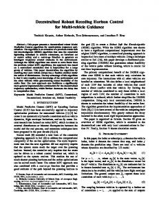
A Monte Carlo simulation was done to assess the effectiveness of the developed controller in each wind condition. Fourty flights, lasting 8 minutes each, were simulated through each Dryden wind scenario. The length of the flights was determined such that local variations in wind speed become negligible and an overall pattern for energy gain/loss becomes evident. For each flight the entire Dryden turbulence field was randomly generated. Table 1 shows a summary of the results. A positive value for ∆e/∆x indicates that the controller in question is able to gain energy on average over the course of the simulated flights. For obvious reasons, a greater value of ∆e/∆x is preferable. This value is also meaningful when compared between the controllers. The goal of this research is to provide the greatest energy gain over a baseline controller, in this case the constant speed controller. Figure 7 shows a comparison between the performance of the two controllers. It is clear from the data presented in Figure 7(b) that in the majority of simulations run in the higher energy gust fields, that the gust energy harvesting controller outperforms the baseline constant airspeed controller. It should be noted that in the low altitude, moderate turbulence wind case, in which the gust energy harvesting controller’s controlling variables were tuned, the aircraft performs the best relative to the constant airspeed controller. In the medium altitude, moderate turbulence wind field, the aircraft as modeled was often able to gain a significant amount of energy in the form of altitude and/or airspeed over the course of a flight as shown in Figure 14. In general, as the turbulence intensity increases the performance of the gust energy harvesting controller relative to the constant speed controller increases. Detailed results for each turbulence condition are shown in figures Figure 11 - Figure 14.


0.3 gust energy harvesting

constant va gust energy harvesting

medium/moderate

0.25

0.2 medium/light

∆(∆ e/∆ x)

∆ e/∆ x

0.55 0.5 0.45 0.4 0.35 0.3 0.25 0.2 0.15 0.1 0.05 0 −0.05 −0.1 −0.15 −0.2 −0.25 −0.3 −0.35 −0.4

low/light

0.15 medium/light 0.1

low/moderate

0.05

low/moderate

low/light 0 medium/moderate −0.05

altitude/turbulence conditions (a) energy change per distance traveled

altitude/turbulence conditions (b) improvement in energy change per distance traveled

Figure 7. A summary of controller performance across four Dryden turbulence conditions. Data was developed in a Monte Carlo simulation of 40 flights for each wind condition, each flight lasting 8 minutes. Subplot 7(a) shows energy change per distance flown for both the baseline constant airspeed controller and the developed gust energy harvesting controller. Subplot 7(b) shows the performance of the gust energy harvesting controller when compared to the constant airspeed controller across all turbulence cases. The star shows the mean value, de while the bars show minimum, maximum and ±1σ. The dotted black line in subfigure 7(a) shows dx for the L aircraft at best D in zero wind.

Figure 11 shows that very little improvement over the baseline constant airspeed controller is gained by utilizing the gust energy harvesting controller in the low altitude, low turbulence condition. The average etot follows a similar trend to that obtained by flight at best L/D airspeed through still air as shown in Figure 11(b). This is likely due to the lack of energy available for exploitation in this turbulence condition. In the more energetic turbulence conditions modeled, moderate to exceptional improvement over the baseline controller may be gained in the majority of simulations. In each of these cases, the input Q is often of a larger magnitude for the gust energy harvesting controller as compared to the constant airspeed controller. C.

Thermal Flight

The single thermal is modeled with vertical wind velocity only using a model presented in Gedeon,8 which is employed in other studies of optimal flight trajectories.14, 21 " 2 # 2 x−x x − x0 −( R 0 ) wz (x) = w0 e 1− (25) R where w0 is the maximum vertical wind speed, x0 is the center of the thermal, and R is the thermal radius. The advantage of this model is that it models a region of sinking air around the rising core of air, a phenomenon observed by glider pilots. The area that is affected by this sink is approximately three times the thermal radius. The profile of a typical thermal as well as a typical path generated by the controller though the thermal are shown in Figure 8 For each simulated flight a field of frozen thermals is generated. The thermal spacing, maximum vertical wind speed, and radius for each thermal are randomly generated according to table 2. The average vertical wind speed is then determined over the entire field, then a bias is applied to the field such that the mean vertical wind speed is zero. This is done to model what is known as environmental sink22 in the atmosphere, 12 of 21 American Institute of Aeronautics and Astronautics Paper 2010-8177

wind speed (m/s)

−4

Q (rad/s)

0

−2 wx

0

wx 2 1

−1

airspeed (m/s)

−2 12 10 8

z (m)

6 −20 0 20 40

0

50

100

150

200

250

300

350

400

x (m)

Figure 8. Typical thermal flight depiction.

Table 2. Parameters for thermal fields used in simulation

variable w0 R xi − xj

range [1 -5] [20 100] 2(Ri + Rj )

description (units) maximum vertical wind speed, positive downwards (m/s) thermal radius (m) inter-thermal spacing

where the amount of air traveling downwards is equivalent to the amount of air traveling upwards in a given region. The result is a slight downwards wind whenever the aircraft is not in an updraft. Through a single thermal,the gust energy harvesting controller slows the aircraft in the upwards moving air and increases airspeed in the downwards moving region. This variable airspeed allows for the controller to compare favorably with the constant airspeed controller. A typical flight is shown in Figure 15. In all cases, the gust harvesting controller is better able to take advantage of the wind speed variation than is the constant speed controller. In addition to the expected behavior, pitching upwards in upwards moving air and pitching nose down in downwards moving air, the controller is able to take advantage of the steep wind gradients when entering a thermal. This is evidenced by the aircraft’s tendency to pitch nose down, gaining airspeed and kinetic energy, as it enters each thermal. The constant speed controller is hindered because it remains at the speed for best L/D at all times. Note that best L/D results in maximum range is still air, but not in moving air. It is unable to increase airspeed to quickly traverse regions of sinking air, nor is it able to decrease airspeed in order to take advantage of bountiful regions of rising air. D.

Discussion

No knowledge of future wind conditions or models of atmospheric phenomenon are required for the presented gust energy harvesting controller to effectively fly through a realistic wind environment. All computations can be done with only local knowledge of wind conditions. This means, however, that an instrument or


wind speed (m/s)

−6 −4 −2 0

etot (m)

2 100

0

−100

−200 0

500

1000

1500

2000

2500

3000

3500

4000

4500

x (m) Figure 9. Flight through a thermal field. The upper plot shows wind velocity (longitudinal in red, and vertical in blue). The lower plot shows total specific energy etot , blue denoting the gust controller and red showing the constant speed controller.

process by which local wind speed may be measured is required. From this data wind speed gradients can be approximated and a sequence of pitch rate inputs calculated to carry the aircraft to the end of the plan horizon while maximizing the reward function presented. Table 3. Run-time data for different Dryden wind fields. Note that the more complex wind fields require more computation time.

Altitude / Intensity Low / Low Low / Moderate Medium / Low Medium / Moderate

mean 0.3588s 0.3318s 0.3201s 0.3916s

σ 0.2573s 0.1737s 0.1687s 0.1447s

To assess the feasibility of running the presented controller in close to real-time, the time to compute a solution for each plan horizon was tracked. The results detailed in Table 3 show that the mean time to compute a pitch-rate spline is on the same order as the length of the control horizon used (TC = 0.28s for all cases. There is not a significant difference in computation time required when turbulence intensity is varied at either altitude. The computations presented here are not on a time scale such that they may be run effectively on an aircraft in flight. What is presented is a simulation done in MATLAB that is not compiled nor necessarily optimized for fast run-times. With some modification, real-time implementation of the presented control method should be possible.

VI.

Conclusion

This paper has presented a method for atmospheric gust energy extraction by small Uninhabited Aerial Vehicles employing a receding horizon control method. The method uses instantaneous measurements of wind speed and gradient to assume wind speed and gradient over a limited time horizon and plans a sequence of pitch rate inputs to maximize a developed reward function over the time horizon. In addition to energy gain per horizontal distance traveled, the reward function includes terms designed to ensure that the aircraft does not compromise its ability to gain energy in later plan horizons. An evolutionary algorithm, CMA-ES, was used in tuning the controlling coefficients in the gust harvesting 14 of 21 American Institute of Aeronautics and Astronautics Paper 2010-8177

controller such that flights, on average, yielded the greatest energy gain. A constant airspeed controller was developed and utilized for comparison purposes. All gust harvesting results are shown in comparison to this controller. Performance was assessed using a longitudinal model of aircraft dynamics for flight through steady winds, randomly generated Dryden wind fields and a field of randomly generated Gedeon thermals. The effectiveness of energy harvesting is dependent on wavelength and magnitude of the gust fields.

References 1 Rayleigh,

J. W. S., “The Sailing Flight of the Albatross,” Nature, Vol. 40, 1889, pp. 34. C. J., “Gust Soaring as a Basis for the Flight of Petrels and Albatrosses (Procellariiformes),” Avian Science, Vol. 2, No. 1, 2002, pp. 1–12. 3 Sachs, G., “Minimum shear wind strength required for dynamic soaring of albatrosses,” Ibis, Vol. 147, 2005, pp. 1–10. 4 Boslough, M. B. E., “Autonomous Dynamic Soaring Platform for Distributed Mobile Sensor Arrays,” Tech. Rep. SAND2002-1986, Sandia National Laboratories, 2002. 5 Allen, M. J. and Lin, V., “Guidance and Control of an Autonomous Soaring Vehicle with Flight Test Results,” AIAA Aerospace Sciences Meeting and Exhibit, AIAA Paper 2007-867, American Institute of Aeronautics and Astronautics, Reno, Nevada, January 2007. 6 Phillips, W. H., “Propulsive Effects due to Flight through Turbulence,” Journal of Aircraft, Vol. 12, No. 7, July 1975, pp. 624–626. 7 Irving, F., “The Energy Loss in Pitching Manoeuvres,” Proceedings of the XVI OSTIV Congress, Organisation Scientifique et Technique Internationale du Vol ` a Voile, 1978. 8 Gedeon, J., “Dynamic Analysis of Dolphin Style Thermal Cross Country Flight,” Proceedings of the XIV OSTIV Congress, Organisation Scientifique et Technique Internationale du Vol a ` Voile, 1974. 9 Zhao, Y. J., “Optimal Patterns of Glider Dynamic Soaring,” Optimal Control Applications and Methods, Vol. 25, No. 2, 2004, pp. 67–89. 10 Zhao, Y. J. and Qi, Y. C., “Minimum Fuel Powered Dynamic Soaring of Unmanned Aerial Vehicles Utilizing Wind Gradients,” Optimal Control Applications and Methods, Vol. 25, No. 5, 2004, pp. 211–233. 11 Lissaman, P., “Wind Energy Extraction by Birds and Flight Vehicles,” 43rd AIAA Aerospace Sciences Meeting and Exhibit, AIAA Paper 2005-241, American Institute of Aeronautics and Astronautics, Reno, Nevada, January 2005. 12 Lissaman, P. B. S. and Patel, C. K., “Neutral Energy Cycles for a Vehicle in Sinusoidal and Turbulent Vertical Gusts,” 45th AIAA Aerospace Sciences Meeting and Exhibit, AIAA Paper 2007-863, American Institute of Aeronautics and Astronautics, Reno, Nevada, January 2007. 13 Patel, C. K. and Kroo, I., “Control Law Design for Improving UAV Performance using Wind Turbulence,” AIAA Aerospace Sciences Meeting and Exhibit, AIAA Paper 2006-0231, American Institute of Aeronautics and Astronautics, Reno, Nevada, January 2006. 14 Langelaan, J. W. and Bramesfeld, G., “Gust Energy Extraction for Mini- and Micro- Uninhabited Aerial Vehicles,” 46th AIAA Aerospace Sciences Meeting and Exhibit, AIAA Paper 2008-0223, American Institute of Aeronautics and Astronautics, Reston, Virginia, January 2008. 15 Lawrance, N. R. J. and Sukkarieh, S., “Wind Energy Based Path Planning for a Small Gliding Unmanned Aerial Vehicle,” AIAA Guidance, Navigation and Controls Conference, American Institute of Aeronautics and Astronautics, Reston, Virginia, August 2009. 16 Langelaan, J. W., “Biologically Inspired Flight Techniques for Small and Micro Unmanned Aerial Vehicles,” AIAA Guidance, Navigation and Control Conference, No. AIAA Paper 2008-6511, American Institute of Aeronautics and Astronautics, Reston, Virginia, August 2008. 17 Hansen, N., “The CMA-Evolution Strategy: A Comparing Review,” Studies in Fuzziness and Soft Computing, Vol. 192, 2006, pp. 75–102. 18 Hansen, N., “The CMA Evolution Strategy: A Tutorial,” Alogrithm Creator’s Website, December 2009, http://www.lri.fr/ hansen/cmatutorial.pdf. 19 “Domino Convergence, Drift, and the Temporal-Salience Structure of Problems,” 1998. 20 “Flying Qualities of Piloted Airplanes,” Military Specification MIL-F-8785C, November 1980. 21 Qi, Y. C. and Zhao, Y. J., “Energy-Efficient Trajectories of Unmanned Aerial Vehicles Flying Through Thermals,” Journal of Aerospace Engineering, Vol. 18, No. 2, April 2005, pp. 84–92. 22 Allen, M. J., “Updraft Model for Development of Autonomous Soaring Uninhabited Air Vehicles,” 44th AIAA Aerospace Sciences Meeting and Exhibit, Reno, Nevada, January 2006. 2 Pennycuick,


Appendix: Vehicle Properties Simulation results are based on the Northeast Sailplane Products Omega II 2M radio control glider. Parameters in Table 4 were obtained from a drag buildup computation, state limits in Table 5 were defined to limit states to “reasonable” bounds. Note that a fourth order polynomial is used to relate CD to CL : this provided a better fit to the computed data over the full speed range. Table 4. Parameters for Omega II 2M glider.

variable m b c S Iyy CL0 CLα CLQ fLD (ϕ)

value 1.31 kg 1.99 m 0.1538 m .3058 m2 .5483 kg.m2 0.1779 5.1681 /rad -2.2189 s/rad 0.1488ϕ4 − 0.2624ϕ3 + 0.1929ϕ2 −0.0511ϕ + 0.0228

description mass span MAC wing area pitch moment of inertia

ϕ = CL0 + CLα α

Table 5. State limits and control saturation for Omega II 2M glider.

state/control θ va α Q

range [−60◦ 60◦ ] [7.5m/s 20m/s] [−5◦ 15◦ ] [−πrad/s πrad/s]

0

description pitch airspeed angle of attack pitch rate

30

−0.5 25

−1

20

−2

CL / CD

h˙ (m/s)

−1.5

−2.5 −3

15 10

−3.5 −4

5

−4.5 −5

0 5

10

15

20

25

va (m/s)

5

10

15

20

25

va (m/s)

(a) Sink rate versus airspeed for the Omega II (b) L/D versus airspeed for the Omega II 2M 2M glider glider

Figure 10. Vehicle properties as modeled


wind speed (m/s)

−7.5 −5 −2.5 0 wx

2.5 5 7.5 −100

wx

z (m)

0 100

airspeed (m/s)

200 15

10

etot (m)

5 100 0 −100

Q (rad/s)

−200 2 1 0 −1 −2

0

500

1000

1500

2000

2500

3000

3500

4000

4500

5000

3500

4000

4500

5000

x (m) (a) Detail of a single run 120

average etot (m)

80 40 0 −40 −80

gust energy harvesting constant airspeed best glide, no wind

−120 −160 −200

0

500

1000

1500

2000

2500

3000

x (m) (b) Mean total energy

Figure 11. A comparison between the developed gust controller and a constant speed controller through a Dryden gust field at low altitude, low turbulence. Subfigure 11(a) shows a detail of a representative single run, 8 minutes in length. The gust energy harvesting controller is shown in blue while the baseline constant airspeed controller is shown in red. Subfigure 11(b) shows the mean total energy over all 40 runs in the Monte Carlo Simulation. Again, the gust energy harvesting controller is shown in blue, while the constant airspeed controller is shown in red. The dotted black line represents glide at best L/D in no wind.


wind speed (m/s)

−7.5 −5 −2.5 0 wx

2.5 5 7.5 −100

wx

z (m)

0 100

airspeed (m/s)

200 20 15 10

etot (m)

5 100 0 −100

Q (rad/s)

−200 2 1 0 −1 −2

0

500

1000

1500

2000

2500

3000

3500

4000

4500

5000

3500

4000

4500

5000


average etot (m)

80 40 0 −40 −80


−120 −160 −200

0

500

1000

1500

2000

2500

3000


Figure 12. A comparison between the developed gust controller and a constant speed controller through a Dryden gust field at low altitude, moderate turbulence. Subfigure 12(a) shows a detail of a representative single run, 8 minutes in length. The gust energy harvesting controller is shown in blue while the baseline constant airspeed controller is shown in red. Subfigure 12(b) shows the mean total energy over all 40 runs in the Monte Carlo Simulation. Again, the gust energy harvesting controller is shown in blue, while the constant airspeed controller is shown in red. The dotted black line represents glide at best L/D in no wind.


wind speed (m/s)

−7.5 −5 −2.5 0 wx

2.5 5 7.5 −200

wx

z (m)

0 200

airspeed (m/s)

400 15

10

etot (m)

5 200 0 −200

Q (rad/s)

−400 2 1 0 −1 −2

0

500

1000

1500

2000

2500

3000

3500

4000

4500

5000

3500

4000

4500

5000


average etot (m)

80 40 0 −40 −80


−120 −160 −200

0

500

1000

1500

2000

2500

3000




wind speed (m/s)

−7.5 −5 −2.5 0 wx

2.5 5 7.5 −1000

wx

z (m)

−500 0

airspeed (m/s)

500 30 20 10

0 1000

etot (m)

500 0

Q (rad/s)

−500 2 1 0 −1 −2

0

500

1000

1500

2000

2500

3000

3500

4000

4500

5000

3500

4000

4500

5000


average etot (m)

80 40 0 −40 −80


−120 −160 −200

0

500

1000

1500

2000

2500

3000




wind speed (m/s)

−6 −4 −2 wx

0

wx

2 −100

z (m)

0 100

airspeed (m/s)

200 15

10

etot (m)

5 100 0 −100

Q (rad/s)

−200 1 0 −1 −2

0

500

1000

1500

2000

2500

3000

3500

4000

4500

5000

x (m)

Figure 15. A comparison between the developed gust controller and a constant speed controller through a randomly generated thermal field. The upper plot shows wind velocity (longitudinal in red, and vertical in blue). The rest of the plots show the gust controller in blue, and the constant airspeed controller in red.
