CLIMATE RESEARCH Clim Res
Vol. 33: 159–169, 2007
Published February 22
Recent California climate variability: spatial and temporal patterns in temperature trends Steve LaDochy1,*, Richard Medina1, 3, William Patzert2 1
Department of Geography & Urban Analysis, California State University, 5151 State University Drive, Los Angeles, California 90032, USA 2
Jet Propulsion Laboratories, NASA, 4800 Oak Grove Drive, Pasadena, California 91109, USA
3
Present address: Department of Geography, University of Utah, 260 South Central Campus Drive, Salt Lake City, Utah 84112-9155, USA
ABSTRACT: With mounting evidence that global warming is taking place, the cause of this warming has come under vigorous scrutiny. Recent studies have lead to a debate over what contributes the most to regional temperature changes. We investigated air temperature patterns in California from 1950 to 2000. Statistical analyses were used to test the significance of temperature trends in California subregions in an attempt to clarify the spatial and temporal patterns of the occurrence and intensities of warming. Most regions showed a stronger increase in minimum temperatures than with mean and maximum temperatures. Areas of intensive urbanization showed the largest positive trends, while rural, non-agricultural regions showed the least warming. Strong correlations between temperatures and Pacific sea surface temperatures (SSTs) particularly Pacific Decadal Oscillation (PDO) values, also account for temperature variability throughout the state. The analysis of 331 state weather stations associated a number of factors with temperature trends, including urbanization, population, Pacific oceanic conditions and elevation. Using climatic division mean temperature trends, the state had an average warming of 0.99°C (1.79°F) over the 1950–2000 period, or 0.20°C (0.36°F) decade–1. Southern California had the highest rates of warming, while the NE Interior Basins division experienced cooling. Large urban sites showed rates over twice those for the state, for the mean maximum temperatures, and over 5 times the state’s mean rate for the minimum temperatures. In comparison, irrigated cropland sites warmed about 0.13°C decade–1 annually, but near 0.40°C for summer and fall minima. Offshore Pacific SSTs warmed 0.09°C decade–1 for the study period. KEY WORDS: Climate variability · California climate · Landuse change Resale or republication not permitted without written consent of the publisher
Most climatologists accept the concept that increasing greenhouse gases may lead to global warming. However, for explaining regional warming, many different causes are cited. Some studies have looked at the role of urbanization and land use changes in causing regional warming (Christy & Goodridge 1995, Dai et al. 1999, Kalnay & Cai 2003, Bereket et al. 2005, Diem et al. 2006). Christy & Norris (2004) argue that irrigation and soil moisture are major contributors, while others favor changes in cloudiness as a principal contributor to regional temperature variability (Henderson-Sellers 1992, Dai et al. 1999, Braganza et al. 2004).
Still others choose the largest geographic feature to the west of California, i.e. the Pacific Ocean. Bratcher & Giese (2002) contend that tropical Pacific sea surface temperatures (SSTs) and their changes precede global air temperatures. On a regional scale, North Pacific SSTs are highly correlated to California temperatures (Hannes & Hannes 1993, LaDochy et al. 2004). California has some of the most diverse microclimates in North America. Its complex topography and large latitudinal extent lead to the whole spectrum of climates, besides tropical. And yet, when speculating on how global warming would impact the state, climate change models and assessments often assume that the influence would be uniform (Hansen et al.
*Email:
[email protected]
© Inter-Research 2007 · www.int-res.com
1. INTRODUCTION
160
Clim Res 33: 159–169, 2007
1998, Hayhoe et al. 2004, Leung et al. 2004). However, uniformity is certainly not the case. In their study of the Central Valley, Christy & Norris (2004) noted that minimum temperatures increased much faster than for maxima in the irrigated farmlands around Fresno from 1930 to 2000. They believe higher moisture levels reduce longwave radiational cooling, while soil moisture and vegetation increase the thermal capacity of the surface. At the same time, enhanced evapotranspiration amounts also lower values of maximum temperatures. But in comparison, hillside and mountainous stations outside the croplands showed more uniform temperatures over time. The largest difference occurred with summer and fall minima when irrigated croplands warmed 0.40°C decade–1, with the annual rate at about 0.13°C decade–1. The rapid growth of the wine industry has added to the irrigated acreage, particularly in the Central Valley where it has nearly doubled since 1950 (Christy & Norris 2004). In the Napa and Sonoma Valleys of northern California, grape growers have benefited from modest warming of 1.13°C from 1951 to 1997 and a 20 d reduction in frost occurrence (Nemani et al. 2001). At the same time, the state’s population has more than doubled, with the fastest growth occurring along the central and southern coasts (US Census 2002). Christy & Goodridge (1995) noted that temperatures over the previous few decades were increasing fastest in counties with the highest population, slower in counties with lower urban populations, and slowest in rural counties. Bereket et al. (2005), in their study of Central Valley urban heat islands, found significant surface temperature increases in locations where rapid urbanization and population growth have taken place. Gallo et al. (1999) found land use differences did cause differences in temperature trends, by comparing rates of warming between urban, suburban and rural stations in the US Historical Climatology Network. Robeson (2004) noted that the lower percentiles of daily minimum temperatures over western and central North America had warmed over 3°C in the last 50 yr during January to March. The more rapid increase in minimum temperatures than maximum temperatures in the last 50 yr has led to decreased diurnal temperature range (DTR) over the USA (Braganza et al. 2004). However, the decrease in DTR is not spatially uniform (Easterling et al. 1997). The recent warming in many parts of North America, as well as elsewhere, is not consistent in time or space. Measuring trends in annual and seasonal temperatures is a common method to view climate variability and change. In the present study we use temperature trends in California climate records over the last 50 yr to measure the extent of warming in the various subregions of the state. By looking at human-induced
changes to the landscape, we attempt to evaluate the importance of these changes with regard to temperature trends, and determine their significance in comparison to those caused by changes in atmospheric composition.
2. METHODS AND DATA Unadjusted annual mean, maximum and minimum temperatures (Tmean, Tmax and Tmin) for 331 California weather stations were used to construct temperature trends from approximately 1950 to 2000. Only stations with long-term, continuous data were used in the analyses. This resulted in 226 stations being used for Tmean, 219 for Tmax and 233 for Tmin. Fig. 1 shows the locations of weather station sites used in the present study, which cover all regions of the state, but with higher representation in the more populous coastal areas and at lower elevations (climatic data were provided by the Western Regional Climate Center; www.wrcc.dri.edu). Although many stations moved over the 50 yr period, annual temperatures were not adjusted. In their analyses of the US Historical Climatology Network (USHCN) temperature database, Balling & Idso (2002) found that trends in unadjusted temperature records are not different from the trends of an independent satellite-based lower tropospheric temperature record or from trends of balloon-based nearsurface measurements. They also strongly suggested that adjustments to the USHCN data set spuriously increase the long-term trend (Balling & Idso 2002). Population data were downloaded by county from the US Census website at www.census.gov, and a population density Geographic Information Systems (GIS) shapefile was created by dividing each county’s population 2000 by the area (sq. mile). The area of each county was provided in a shapefile downloaded from the United States Geological Survey (USGS) website at www.usgs.gov. The California Urban Areas 2000 GIS data were also downloaded from the US Census website. The National Climatic Data Center, NCDC, collects climatic data by climate divisions for each state. Each division pools together stations that have comparable climatic controls, that is, stations are as near as possible climatically homogenous. For California, there are 7 recognized climatic divisions, each averaging several cooperative stations, including urban, suburban and rural sites (climatic division data available at www.cdc.noaa.gov/USclimate/USclimdivs.html). Annual Tmean by climatic divisions were used to calculate divisional temperature trends for the 1950–2000 period. Using an area-weighting technique in which we summed each division’s temperature trend,
LaDochy et al.: California climate variability
161
Fig. 1. Study area (California, USA) showing location of the 331 weather stations used
weighted (multiplied) by its proportional area of the state, we derived the state arithmetic Tmean trend. To create rates of change for California regions during the 1950–2000 period, we used simple linear regression for each of the long-term data stations, where the slope was assumed to be the rate of change. Rates of change were created in this fashion for the 3 temperature averages (Tmean, Tmax, Tmin). The slopes, or rates of change, for each station were then mapped and overlaid onto the ‘County population density 2000’, and ‘Urban areas 2000’ basemaps. Tmean
rates for stations falling into the urban areas for 2000 are compared with stations that are non-urban using a difference of means t-test. Monthly and seasonal rates of change were calculated for the Los Angeles Civic Center to investigate urban heat island patterns. Temperature rates of change were also classified into 3 groups by elevation: low (0 to 250 m), middle (251 to 500 m), and high (> 500 m). Most (237) stations fell into the low category, with 64 in the middle and 28 in the high group. Comparisons were made between the low category and the other groups.
162
Clim Res 33: 159–169, 2007
Fig. 2. Distribution of mean temperature (Tmean) trends (°C decade–1), California, 1950–2000
To look at the influence of oceanic or climatic indices, especially Pacific SSTs, annual Tmean, Tmax and Tmin were correlated with annual PDO (Pacific Decadal Oscillation), SOI (Southern Oscillation Index), NP (North Pacific Index) and AO (Arctic Oscillation) for the 50 yr period (available from www.cdc.noaa.gov/ ClimateIndices/). The strengths of the correlations were mapped to show the spatial distribution of correlation values.
3. RESULTS AND DISCUSSION 3.1. Mean temperature By testing the average Tmean of stations for significant change, it was established that approximately 59% or 129 of the 226 weather stations in California showed significant change at 95% confidence. The other 41% were assumed to have no significant
163
LaDochy et al.: California climate variability
Table 1. t-test for mean rates of temperature change decade–1 (urban and non-urban stations). SD: standard deviation, SE: standard error, diff.: difference
Urban Non-urban
N
Mean
SD
SE
99 121
0.1970 0.0764
0.1483 0.1499
0.0149 0.0136
t
Equal variance 5.963 assumed
df
218
p Mean (2-tailed) diff. 0.000
0.12056
SE diff. 0.02022
3.2. Maximum temperature Of the 219 stations tested for Tmax, 94 were found to have significant rates of change from 1950–2000, which is 43% of the total. Again the other 57% were mapped as ‘no change’. The portion of the 94 stations that had significant rates of change as positive is 66 or 70%, while 30% of those stations had negative rates of change. By looking at average Tmax draped over the urban-areas map (Fig. 4), the warming is not as apparent as it is with average (Fig. 2) and average Tmin (see Fig. 5) temperatures, with some urban areas even showing decreases. The majority of the stations shown in Fig. 4 have either no significant rate of change or negative values. In southern California, while none of the stations show decreasing Tmean, there are several stations showing decreases for Tmax. Several studies of urban heat islands show that maximum temperatures are either only slightly warmer than their surrounding rural environments, or even cooler (Mitchell 1961, Oke 1995).
Change (°C)
Div. 1 0.23
0.2
Div. 3 -0.12 Div. 2 0.12
N e v a
Div. 5 0.17
P
d
Div. 4 0.17
a
a
c i
Div. 7 0.29
f
i
change, and mapped as such. Of the 129 stations, 8 (6%) show a decrease in Tmean during the last 50 yr while 121 (94%) show an increase. In Fig. 2, these results are overlaid on an urban-areas map using graduated symbols to show the rate of temperature change per decade. We can see that the 8 negative stations are located in the center and northeast part of the state, mainly rural, while the majority of coastal stations (mostly urban) are positive. A majority of the stations in or surrounding the 2 most heavily populated areas (Los Angeles Basin and the Bay Area) also show some of the fastest rates. Differences in mean rates of temperature change between stations designated as urban and those outside urban areas were significantly different (Table 1). The urban stations had a significantly (p = 0.000) higher mean decadal rate of temperature change (0.20 to 0.08), with a t value of 5.96, than nonurban stations. With such a diversity of climate regions, one would expect large differences in temperature trends simply due to terrain/albedo differences. Fig. 3 shows the Tmean trends for climatic divisions during 1950–2000. The statewide rate of warming for the period of record is 0.20°C decade–1. That is about half of the 0.39°C decade–1 rate for North America surface temperatures calculated by Jones et al. (1999), using in situ data between 1981 and 2003, while AVHRR (advanced very high resolution radiometer) data for the same period recorded 0.79°C decade–1 warming (Comiso & Parkinson 2004). However, California values correspond more closely to rates calculated for US land use categories during 1950–1996 by Gallo et al. (1999). Only the NE Interior Basins division shows a decrease in temperatures. The 2 Central Valley divisions show the slowest increase in temperatures, with faster warming along the coast, and the fastest warming in the SE Desert Basin. The latter climatic division is dominated by some of the fastest growing inland urban areas, such as Riverside and San Bernardino, and resort areas such as Palm Springs. Of the coastal divisions, the heavily urbanized south coast has the highest warming
rates. In comparing Figs. 2 & 3, the notion that climatic divisions represent regions of uniform climatic controls may be questioned.
c
O
100 50
0
c
e
100
a 200
Div. 6 0.25
n 300
Kilometers
Fig. 3. Mean temperature trends (Tmean) (°C decade–1) by climatic division, California, 1950–2000. Source: National Climatic Data Center, NOAA
164
Clim Res 33: 159–169, 2007
Fig. 4. Distribution of maximum temperature trends (Tmax) (°C decade–1), California, 1950–2000
3.3. Minimum temperature and diurnal temperature range With respect to the stations’ average Tmin, 142 of the 233 selected stations (61%) have significant rates of change, which is higher than the other 2 categories. The other 39% were mapped as ‘no change’. Of the 142 stations with significant change, 129 or 91% are changing at a positive rate, while only 9% are nega-
tive. Overlaid on the urban-areas map, Fig. 5 shows the close relationship of increasing temperatures with urban land use, not just in populous counties. For example, San Diego, Riverside and San Bernardino counties all show high rates of temperature increase in urban areas, but insignificant change in the more rural eastern portions of their counties. In general, Tmin are increasing faster than Tmean and Tmax. California temperature trends, like the rest of North America,
LaDochy et al.: California climate variability
165
Fig. 5. Distribution of minimum temperature trends (Tmin) (°C decade–1), California, 1950–2000
show decreasing diurnal temperature range (DTR) for many of the stations. Of the 219 stations with sufficient DTR rate of change data, 102 (46.6%) have negative rates of change, only 30 (13.7%) have positive rates, while 87 (39.7%) have no significant change. Urbanization seems to be a major contributor to station temperature increases, with average Tmin often rising twice that of average Tmax, similar to other regions of the U.S. (Gallo et al. 1999). Los Angeles Civic Center
shows that Tmin have increased 5°C since 1878, while Tmax only about 2°C in the same period (Fig. 6). The largest increases in minimum temperatures occur in summer and fall, with lowest rates in winter (not shown). Los Angeles maximum temperatures increased fastest in winter and slowest in summer and fall, or nearly the opposite to minimum temperatures (not shown). Christy & Norris (2004) found similar results for the irrigated Central Valley. However, neg-
166
Clim Res 33: 159–169, 2007
30.0 Average maximum temperature (
)
y = 0.0141x + 22.338
Temperature change = +1.67°C
Average minimum temperature (
)
y = 0.0328x + 10.519
Temperature change = +4.00°C
Tmax minus Tmin temperature (
)
y = – 0.0187x + 11.819
Temperature change = –2.33°C
Temperature (°C)
25.0
20.0
15.0
10.0
1878 1882 1886 1890 1894 1898 1902 1906 1910 1914 1918 1922 1926 1930 1934 1938 1942 1946 1950 1954 1958 1962 1966 1970 1974 1978 1982 1986 1990 1994 1998 2002
5.0
Year ative DTR rates are not seen in less populated regions. Fig. 7 shows only a small number of rural stations with increases in DTR. Precipitation has not increased significantly for most California stations in the 1950–2000 period (not shown), although there were more wet El Niño years during the warm phase of the PDO from about 1977 to 1997 than in the previous cool phase, covering the 1950–1976 half of the study period. It does not seem as though precipitation and increases in cloudiness have contributed as much as urbanization to the decreases in DTR. In comparison to Tmean and Tmax, Tmin rates were also highest for each of the 3 elevation categories: low (≤ 250 m), middle (251–500 m), and high (> 500 m). The lowest elevation stations had the highest rates for Tmean, Tmin and Tmax. Oddly, the high elevation stations had higher rates than those of middle stations. However, the sample sizes for middle and high elevation stations were much lower, with only 17 high stations having long-term data for all 3 temperature categories. Combining the 2 higher elevation categories into one ‘high’ category, a comparison can be made between annual Tmean rates for low vs. high. Using a t-test for differences in means, there is a statistically significant difference between the stations at the 2 elevation categories. The test shows that the low category has a significantly higher mean decadal temperature rate (0.15) than the combined high category (0.08), with a t-value of 3.29 (p = 0.001) (Table 2). Table 2. t-test for differences in mean rates of temperature change for station elevations Elevation Low (< 250 m) High (> 250 m)
N
Mean
t
p (2-tailed)
154 66
0.15 0.08
3.294
0.001
Fig. 6. Los Angeles Civic Center trends in Tmax and Tmin and diurnal temperature range (‘DTR; Tmax– Tmin), 1878–2003
3.4. Temperatures and oceanic and climatic indices Bivariate correlation was utilized for each of the climate stations and the oceanic/atmospheric indices, using all long-term data stations in order to determine correlation between average annual air temperature and PDO (Jones, et al. 1999), NP, SOI, and AO. There is a significant positive correlation between average Tmean and PDO. This means that positive (negative) PDO, which is the warm (cold) phase, relates with higher (lower) air temperatures. Additionally, the analysis suggests a significant negative correlation between average Tmean and NP. Higher (lower) NP values, which occur when there is a stronger (weaker) North Pacific High, relate to lower (higher) air temperatures. Our analysis showed that only a handful of stations revealed a significant negative correlation between Tmean and the SOI, i.e. when positive (negative) SOI conditions — or those tending towards La Niña (El Niño) — occur, air temperatures are lower (higher). Correlations between Tmean and AO were mostly non-significant. These results match those found by LaDochy et al. (2004) and Alfaro et al. (2004) correlating temperatures for climatic divisions along the west coast with Pacific indices. They noted that the PDO was the best variable for explaining temperature variability along the California coast, and showed a significant positive correlation. Fig. 8 shows the spatial distributions of correlations between PDO values and mean temperature rates. It is apparent that the majority of the climate stations correlate positively with PDO values. While 168 of the 220 (76%) stations with sufficient data correlate significantly with PDO, only one station correlated negatively, South Entrance Yosemite National Park. For the correlation between average Tmax and PDO, the majority of stations do not correlate (not shown).
LaDochy et al.: California climate variability
167
Fig. 7. Distribution of diurnal temperature range trends (DTR) (°C decade–1), California, 1950–2000
Only 96 of 219 (44%) correlate significantly, and 3 of these stations, Calaveras Big Trees, Potter Valley PH, and South Entrance Yosemite National Park, correlate negatively. With the average Tmin and PDO, station values have the highest percentage of significantly correlated stations at 83% or 193 of 233 stations, all positively correlated (not shown). The highest concentration of correlated stations, and the strongest correlations, appears to be along the coast, in general.
Pacific SSTs also show a tendency of warming, especially near the California coast (not shown). These temperatures, while showing an upward trend, also reflect SOI extremes and PDO phase changes (LaDochy et al. 2004). Although not impressive, coastal SST rates are still over half the warming rate calculated for Central Valley irrigated agricultural land by Christy & Norris (2004). Nemani et al. (2001) show that warming coastal waters relate to increased humidity and nighttime cloud cover near the coast, which accounts for the
168
Clim Res 33: 159–169, 2007
Fig. 8. Distribution of correlations between minimum temperature (Tmean) and Pacific Decadal Oscillation (PDO) values, California, 1950–2000
faster warming of Tmin and decreasing DTR for the Napa and Sonoma Valleys.
4. CONCLUSIONS Temperatures increased during 1950–2000 for much of the state, with minimum temperatures increasing faster than maxima, leading to reduced DTR. However there are great variations in these patterns within
subregions that seem to point to land-use change as the main control. Some of the largest temperature increases occur in the vicinity of urban centers, particularly for minimum temperatures. Few rural stations show significant increases in minimum or maximum temperatures. An exception may be some agricultural sites, where minimum temperatures show increases comparable to some urban areas. While few stations showed temperature decreases for mean and minimum rates, there were substantial numbers of stations
LaDochy et al.: California climate variability
showing decreases in maximum temperatures, including some urban sites. If we assume that global warming affects all regions of the state, then the small increases seen in rural stations can be an estimate of this general warming pattern over land. Larger increases must then be due to local or regional surface changes. Using climatic division data, the fastest rates of warming were recorded in the southern California divisions, where urbanization has been greatest. The least warming occurred in the Central Valley, with the more irrigated south (San Joaquin drainage) having greater warming than the less irrigated north (Sacramento drainage). The NE Interior Basins division had cooling over the period of record, although most stations in the northern divisions had insignificant rates of change. It is unfortunate that the period of record is so short, especially since it practically overlays the switching from the cool phase to the warm phase of the PDO, which is highly correlated to temperatures statewide. Therefore, warming due to higher coastal sea surface temperatures since the shift around 1977 (Deser et al. 1996) should have increased temperatures, both minimum and maximum. SST rates offshore have increased at about half the rate of warming of the state, using climatic division data. The amount of this contribution interferes with calculating the background global warming signal and the magnitude of land-use change contributions.
169
Alfaro E, Gershunov A, Cayan D, Steinemann A, Pierce D, Barnett T (2004) A method for prediction of California summer air surface temperature. Eos Trans Am Geophys Union 85:553, 557–558 Balling RC Jr, Idso CD (2002) Analysis of adjustments to the United States Historical Climatology Network (USHCN) temperature database. Geophys Res Lett 29(10):25-1–25-3 doi:10.1029/2002GL014825 Bereket L, Fabris D, Gonzalez JE, Chiappari S, Zarantonello S, Miller NL, Bornstein R (2005) Climatology temperature mapping for California urban heat island study site selection. Paper 6.4, Am Meteorol Soc Atmos Sci Air Qual Conf, San Francisco, CA, 27–29 April Braganza L, Karoly DJ, Arblaster, JM (2004) Diurnal temperature range as an index of global climate during the twentieth century. Geophys Res Lett 31(13):doi:10.1029/ 2004GL019998 Bratcher AJ, Giese BS (2002) Tropical Pacific decadal variability and global warming. Geophys Res Lett 29(19):24-1– 24-4 doi:10.1029/2002GL015191 Christy J, Norris WB (2004) Irrigation-induced warming in central California? Proc Am Meteorol Soc 14th Conf
on Appl Climatol, Seattle, WA, January 12–16, American Meteorological Society, Boston Christy JR, Goodridge J (1995) Precision global temperatures from satellites and urban warming effects of non-satellite data. Atmos Environ 29:1957–1961 Comiso JC, Parkinson CL (2004) Satellite-observed changes in the arctic. Phys Today 57:38–44 Dai A, Trenberth KE, Karl TR (1999) Effects of clouds, soil moisture and water vapor on diurnal temperature range. J Clim 12:2451–2473 Deser C, Alexander MA, Timlin MS (1996) Upper ocean thermal variations in the North Pacific. J Clim 9:1840–1855 Diem JE, Ricketts CE, Dean JR (2006) Impacts of urbanization on land-atmosphere carbon exchange within a metropolitan area in the USA. Clim Res 30:201–213 Easterling DR, Horton B, Jones PD, Peterson TC and 7 others (1997) Maximum and minimum temperature trends for the globe. Science 277:364–367 Gallo KP, Owen TW, Easterling DR, Jamason PF (1999) Temperature trends of the US Historical Climatology Network based on satellite-designated land use/land cover. J Clim 12:1344–1348 Goodridge JD (1996) Comments on ‘Regional simulations of greenhouse warming including national variability’. Bull Am Meteorol Soc 77:1588–1589 Hannes PH, Hannes SM (1993) Pacific Ocean air interactions: California seasonal air temperatures versus ocean temperatures. Calif Geogr 33:3–13 Hansen J, Sato M, Glascoe J, Ruedy R (1998) A commonsense climatic index: Is climate change noticeable? Proc Nat Acad Sci 95:4113–4120 Hayhoe K, Cayan D, Field CB, Frumhoff PC and 15 others (2004) Emissions, pathways, climate change, and impacts on California. Proc Nat Acad Sci 101(34):12422–12427 doi:10.1073/pnas.0404500101 Henderson-Sellers A (1992) Continental cloudiness changes this century. GeoJournal 27:255–262 Jones PD, Horton EB, Folland CK, Hulme M, Parker DE, Barnett TA (1999) The use of indices to identify changes in climatic extremes. Clim Change 42:131–149 Kalnay E, Cai M (2003) Impact of urbanization and land-use change on climate. Nature 423:528–531 LaDochy S, Brown J, Selke M, Patzert W (2004) Can US West Coast climate be forecast? Proc Am Meteorol Soc Symp on Forecasting Weather and Clim of the Atmos and Ocean, Seattle, WA, Jan 11–14. American Meteorological Society, Boston. Available at: http://ams.confex.com/ams/pdfpapers/ 71130.pdf Leung LR, Qian Y, Bian X, Washington WM, Han J, Roads JO (2004) Mid-century ensemble regional climate change scenarios for the western United States. Clim Change 62:75–113 Mitchell JM, Jr (1961) The temperature of cities. Weatherwise 14:224–229 Nemani RR, White MA, Cayan DR, Jones GV, Running SW, Coughlan JC, Peterson DL (2001) Asymmetric warming over coastal California and its impact on the premium wine industry. Clim Res 19:25–34 Oke TR (1995) The heat island of the urban boundary layer: characteristics, causes and effects. In: Cermak JE, Davenport AG, Plate EJ, Viegas DX (eds) Wind climate in cities. Kluwer Academic, Dordrecht, p 81–107 Robeson SM (2004) Trends in time-varying percentiles of daily minimum and maximum temperature over North America. Geophys Res Lett 31(10): doi:1029/2003GL019019 US Census (2002) US census: historical-California population. Available at http://factfinder.census.gov
Editorial responsibility: Gregory Jones, Ashland, Oregon, USA
Submitted: April 27, 2005; Accepted: October 11, 2006 Proofs received from author(s): January 21, 2007
Acknowledgement. The authors appreciate the help of Cathy Smith, the Climate Diagnostics Center (CDC), Tom Peterson and the NCDC for providing data for this study, Jeff Brown, Peter Chu and Sona Sarian, for early data analyses, and the Jet Propulsion Laboratory NASA for support. We also appreciate the helpful suggestions of the reviewers. LITERATURE CITED