Reduced Size Harmony Search Algorithm for Optimization - Journal of ...

Journal of Electrical Engineering www.jee.ro

Reduced Size Harmony Search Algorithm for Optimization M. OMAR M. A.EBRAHIM [email protected] [email protected] A. M. ABDEL GHANY F.Bendary [email protected] [email protected] Faculty of Engineering at Shoubra, Benha University, Electrical Engineering Department, 108 Shoubra st, Cairo, Egypt. Abstract: This paper introduces a step towards enhancing the performance of an existing AI-technique known as Harmony Search (HS). The original HS suffers from some disadvantages and shortages which motivate the researchers to develop newest variants as will be seen later. Each variant tries to solve and overcome the shortages of the previous one but still leave some shortages behind it. Here, the research work had been devoted to merge all the advantages of HS variants together, and the disadvantages of them had been excluded to introduce a novel technique which is more effective in the optimization problems. The proposed novel optimization technique is applied to design local PID controller for Load Frequency Control (LFC) single area power system. Comparative study is carried out between the basic HS variants and the proposed one using diverse tests in case of linear and nonlinear systems to reveal the robustness and effectiveness of the proposed algorithm. Key words: Harmony search, Optimization, Objective Function, Load Frequency Control. Nomenclature: HM: Harmony memory HMS: Harmony memory size HMCR: Harmony memory consideration rate BW (i): Band width of generation i BWcompensative: Compensative band width PAR (i): Pitch adjusting rate of generation i UB, LB: Upper and lower bounds of variables NI : Number of iterations R: Speed regulation Kp: Power system gain Tg: Governor time constant Tt: Turbine time constant Tp: Power system time constant

1. Introduction. The harmony search (HS) algorithm is considered as a new population-based metaheuristic optimization technique. Itsimulates the improvisation process where musicians improvise their instruments pitch searching for a perfect state of harmony. The HS had attracted many researchers’ from various fields working on solving optimization problems. The improvements which had been applied to the HS algorithm had two ways:

(1) improvements in terms of parameters setting, and (2) improvements in terms of hybridizing HS components with other metaheuristic algorithms [1]. The first way focuses on the optimal selection of the HS parameters values and formulations; this way requires more mathematical and logical requirements in the researcher to be able to modify the algorithm of this optimization method. The second way focuses on hybridizing the HS with other artificial intelligence techniques, by mixing the advantages of each technique into a newest one. The paper is organized as follows: a brief description for HS variants is illustrated in Section 2. Section 3 will focus on the modeling and identification of the proposed novel technique. In Section 4, simulation and results obtained after the application of RSHS algorithm. The main conclusions are driven in section 5. 2. Harmony Search Algorithm HS was proposed by Zong Woo Geem in 2001[2]. It is well known that HS is a phenomenonmimicking algorithm inspired by the improvisation process of musicians. In the HS algorithm, each musician (decision variable) plays a note for finding a best harmony (global optimum) all together. The analogy between improvisation and optimization is likely as follows [2]: 1. Each musician corresponds to each decision variable. 2. Musical instrument’s pitch range corresponds to the decision variable’s value range. 3. Musical harmony at a certain time corresponds to the solution vector at certain iteration. 4. Audience’s aesthetics corresponds to the objective function to be minimized or maximized. In this section, a brief review of HS algorithm and its variants is given. 2.1 The Basic Harmony Search Algorithm In the basic HS algorithm each solution is called a harmony and represented by an n-dimension real vector. An initial population of harmony vectors is randomly generated and stored in a harmony memory (HM). Then a new candidate harmony is generated from all of the solutions in the HM by

1


using a memory consideration rule, a pitch adjustment rule and a random re-initialization. Finally, the HM is updated by comparing the new candidate harmony and the worst harmony vector in the HM. The worst harmony vector is replaced by the new candidate vector if it is better than the worst harmony vector in the HM. The above process is repeated until a certain termination criterion is met. The basic HS algorithm consists of three basic phases, namely, initialization, improvisation of a harmony vector and updating the HM [3]. The steps of the solution are illustrated in the flow chart given in Fig. (1) as follows: Step 1: initialize the HS parameters. Step 2: generate random vectors (X1,…., XHMS) as many as HMS (Harmony Memory Size), then store them in harmony memory (HM) in matrix form, and evaluate the fitness function corresponding to each solution vector:

X11 HM=

. . X1

. . .

Step 1 Initialize all algorithm parameters: HMCR, HMS, PAR, NI, BW, UB, LB

Step 2 Initialize and generate the HM and the corresponding fitness function.

Step 3 Improvise new solution vector based on 3 rules, memory consideration, pitch adjusting, and randomization. For i= 1:NI

Xn1

No rand˂HMCR

Random selection

Yes HMS

Xn

HMS

Memory consideration

Step 4: If Xi' is better than the worst vector X worst in HM, replace Xworst with Xi'. Step 5: Repeat from Step 2 to Step 4 until termination criterion (e.g. maximum iterations) is satisfied. 2.2 The Improved Harmony Search (IHS) The IHS algorithm addresses the shortcomings of the basic HS algorithm which uses fixed values for PAR and BW parameters [4]. The IHS algorithm applies the same memory consideration, pitch adjustment and random selection as the basic HS algorithm, but dynamically updates values of PAR and BW as shown below:

Do nothing

rand˂PAR

Yes

Step 3: Improvise a new harmony from the HM with probability HMCR (0 ≤ HMCR≤ 1), pick the stored value from HM, after that, and with probability of PAR (0 ≤ PAR≤ 1), adjust the selected solution with the band width value according to the following relation: (1)

No

Xi’= Xi’+ rand* BW

Step 4 Yes

Does the new solution is better than the worst one?

Replace the worst solution.

No

Step 5 Termination criteria satisfied?

Yes Stop

Fig.1. Optimization procedure of the Harmony Search algorithm.

2


()

(2)

by Eq. (6) in order to avoid getting trapped in a locally optimal solution.

() (

()

)

(3)

2.3 Global Best Harmony Search (GHS) Inspired by the particle swarm optimization [5], a GHS algorithm that modifies the pitch adjustment rule has been proposed [6]. Unlike the basic HS algorithm, the GHS algorithm generates a new harmony vector XB = {xB(1), xB(2),…., xB(n) } in the HM. The pitch adjustment rule is given as below:

()

( )

(4)

where k is a random integer between 1 and n. In addition, the GHS algorithm employs the dynamic updating procedure for the PAR parameter, Eq. (4). It is claimed that the modified pitch adjustment allows the GHS algorithm to work more efficiently on both continuous and discrete problems. The advantage of this algorithm is that it selects the global best solution every generation as it is without any adjustment to the values of the variables. 2.4 Self Adaptive GHS (SGHS) An extension of the GHS algorithm, a selfadaptive GHS (SGHS) algorithm is presented in this section. Unlike the GHS algorithm, the SGHS algorithm employs a new improvisation scheme and an adaptive parameter tuning method. The GHS algorithm takes advantage of the best harmony vector XB to produce a new vector Xnew. However, the modified pitch adjustment rule may break the building structures in XB, so that Xnew may become worse than Xb with a high probability when solving problems with a global optimum having different numerical values for different dimensions. Therefore, to better inherit good information from XB, a modified pitch adjusting rule is presented as:

()

()

(5)

It should be noted that, according to the modified pitch adjustment rule xnew(j),is assigned to the corresponding decision variable xB (j) in XB, while in the GHS algorithm, xnew(j) is determined randomly by selecting amongst any one of the decision variables of XB [7]. In addition, in the memory consideration phase, the equation in GHS is replaced

()

(6)

In the SGHS algorithm, four control parameters HMS, HMCR, PAR and BW are closely related to the problem being solved and the phase of the search process that may be either exploration or exploitation. These parameters are either learnt or dynamically adapted with respect to the favorable evolution of the search process [2]. These four types of HS are the most popular and commonly used in the different optimization problems, also, there are other types not listed here, had been worked out by researchers, all these types deal with the parameter setting and formulation. 3. Proposed Method (RSHS) All the above variants of HS technique suffers from common shortage when the condition of PAR doesn’t achieved, the algorithm do nothing, this may make the algorithm to generate a solution which is already existing before, so, this iteration will be valueless one. The solution to this problem had been introduced by adjusting the selected solution by a value of BW with probability of PAR, and adjusting it by a value of BWcompensative with probability of (1PAR), this is the first new addition and modification in the proposed algorithm. It will guarantee that there is no any solution will appear twice during the optimization process. The new parameter BWcompensative, had been selected to be a small value about (0.1* BW). The cause behind the selection of this value is that, the original HS type doesn’t give us the authority to adjust the solution vector when the condition of PAR doesn’t achieved, so, it had been decideded to make this value small relative to the BW value, after many trials it had been found that this is the optimal value for the BWcompensative. The second modification applied to the proposed algorithm is to make the HMS linearly decreasing with iterations after 50% of iterations had been completed, and starting from HMSmax until reaches HMSmin as shown in Fig. 2. In this study it is assumed that the number of iterations is 100 and the values of HMSmax and HMSmin are 40, 30 respectively. In the linearly decreasing period of the HMS, the algorithm performs two tasks, namely, replacing and removing, it replaces the worst solution with the current one if it is better, after doing this task the algorithm sorts the fitness function and the corresponding HM solution vectors.

3


Then it makes the removing process by eliminating the worst solution in the HM matrix, now the HMS will be reduced by 1 and it is ready to the next iteration. The elimination of two worst solutions in the same iteration rapids the solution process and makes the convergence of the solution takes place earlier. It had been found that the results are slightly affected by the value of HMSmin. The solution time required by using this method is expected to be less than any other HS variants. When using this proposed method, user should take care from two points: Firstly: The iterations number should be greater than the value of ½ iterations+(HMSmax- HMSmin), usually this is achieved. Secondly: if the fitness function (termination criterion) had been achieved before 50% of iterations number, then the reduction of the HMS will not be used, usually this is not achieved because the fitness function is adjusted to be a very small value.

40

HMS

Step 2: Initialize and generate the HM and the corresponding fitness function. Step 3: Initialize and generate the HM and the corresponding fitness function as follows: For i=1:NI if (rand < HMCR) ,where rand is a random number (0,1) xnew(j) = xB(j) if (rand< PAR) xnew (j) = xnew(j) ± rand*BW else xnew (j) = xnew(j) ± rand*BWcompensative end if else xnew(j) = LBj + r _ (UBj _ LBj) end if end for Step 4: If f(xnew) < f(xW), Update the HM as xnew.

50

HMSmax

Step 6: if (i >½ NI+(HMSmax-HMSmin) continue with HMS min else continue with HMS max, then go to step 3 endif

20 10

1/2 iterations 1/2iterations+(HMSmax- HMSmin) 10

20

30

40

50 60 iteration

70

xW =

Step 5: reduce the HMS as follows: If ( ½NI ≤ i ≤ ½NI+(HMSmax-HMSmin)) Remove the worst solution and corresponding fitness function else go to step 6

HMSmin

30

0 0

The Computational procedure of RSHS is shown in Fig.3 and can be summarized as follows: Step 1: initialize all parameters, HMCR, BW, BW compensative, NI, PAR, UB, LB.

80

90

100

Fig.2. HMS arrangement for the proposed method.

The name of this method came out from the concept of reduction of the HMS with iterations, so it is called RSHS. The new proposed method achieved two advantages, firstly avoiding the repetition of any solution vector during the iteration process, secondly rapids the convergence process by replacing and eliminating the worst solution from the HM matrix.

Step 7: If NI is completed, return the best harmony vector XB in the HM; otherwise go back to step3. 4. Simulation Results In this section, a simple load frequency control model, which is commonly used in the control applications and problems, was chosen to compare the performance of proposed method against the early discussed four variants of HS, namely basic HS, IHS, GHS, and SGHS. The model is realistic due to the presence of nonlinearities. The process is to optimize the three variables of PID controller, kp, ki and kd.

4


Step 1

Step 2

Initialize all algorithm parameters: HMCR, HMS, PAR, NI, BW, UB,LB, HMSmax, HMSmin, BWcompensative

Initialize and generate the HM and the corresponding fitness function.

Step 3 Improvise new solution vector based on 3 rules, memory consideration, pitch adjusting, and randomization. For i= 1:NI

No

Random selection

rand ˂ HMCR Yes

No

Memory consideration

rand ˂ PAR

Xi’= Xi’+ rand* BWcomp

Yes Xi’= Xi’+ rand* BW

Continue with HMSmax

Yes

Does the new solution is better than the worst one?

No

Step 6 i > ½ NI+ (HMSmax-HMSmin)

No

Step 4 Replace the worst solution.

No

Step 5

½ NI ≤ i ≤ ½ NI+ (HMSmax-HMSmin) Yes

Yes Continue with HMSmin

Remove the worst solution and corresponding fitness function

Step 7 Termination criteria satisfied?

No

Yes Stop Fig.3. Flow chart for the RSHS method

5


4.1 Model under Study The model is a nonlinear single area power system. The main target is to optimize the feedback PID controller with the following structure [8]:

( )

(7)

With certain fitness function (J) which is the integrated square error (ISE) of the frequency deviation as given below:

∫ ( ( ) )

(8)

The parameters of each type of HS variants had been listed in Table.1 [9].

For fair comparison, the parameters had been fixed for all algorithms. From the table it is shown that the proposed method has the same parameters values as the basic HS type, in addition to these parameters are BWcompensative, HMSmax and HMSmin. The PID parameters values for all types had been recorded in Table. 2, also the values of running time and fitness function values had been listed in the same table. From these results it is shown that the proposed method (RSHS) has greater fitness function over all other HS variants, and less running time at all. It was expected earlier that the running time will be reduced because the RSHS algorithm completes the optimization process with HMS equal to 30 starting from the iteration number ½ iterations + (HMSmax- HMSmin), rather than 40.

Table.1 parameters value for all HS variants parameter

HMCR

NI

PAR

PARmin

PARmax

BW

Bwcompensative

Bwmin

Bwmax

HMS

HMSmin

HMSmax

HS

0.98

100

0.3

NA

NA

0.1

NA

NA

NA

40

NA

NA

IHS

0.98

100

NA

0.01

0.99

NA

NA

0.001

0.01

40

NA

NA

GHS

0.98

100

0.3

NA

NA

NA

NA

NA

NA

40

NA

NA

SGHS

0.98

100

0.9

NA

NA

NA

NA

0.001

0.01

40

NA

NA

RSHS

0.98

100

0.3

NA

NA

0.1

0.01

NA

NA

NA

40

30

method

Table.2 parameters evaluation for all HS variants based PID parameter

PID gains

Fitness function

Running time (sec)

Reduction in algorithm running time will be significant and more effective in the large problems including large number of variables to be optimized; it is depending mainly on the formulas, loops and equations in the code of each type. The running time had been measured using the Matlab built in functions (tic toc).

method

kp

Ki

kd

HS

0.7957

0.4683

0.4414

0.0019

217

IHS

0.7351

0.5223

0.5984

0.0018

233

GHS

0.8351

0.5316

0.6422

0.0016

208

Case 1: 1% load increment for linear model.

SGHS

0.8442

0.7258

0.7324

0.0015

225

RSHS

0.9161

0.9382

0.9300

0.0015

195

The system had been tested for a step load increment ΔPL = 1%, as shown in Fig. 4 [10].

6


Table.3 response evaluation for all HS variants based PID

ΔPL

Method

HS

IHS

GHS

SGHS

RSHS

% Under shoot

0.779

0.652

0.617

0.572

0.474

Peak time

0.249

0.219

0.215

0.176

0.15

13

11.5

12.5

11.5

11.3

Parameter Turbine

Governor

Rotating Mass

1/R

PID

Settling time

PID Controller

Fig.4. Simulink model under study for case 1

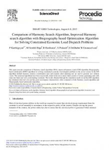
The frequency deviation response with time is shown Fig.5. It is obvious that the RSHS based PID has the best performance among the all HS variants based PIDs, where the system response has the smallest undershoot, peak time and settling time (in seconds) in the case of RSHS based PID as given in Table.3. The reduction in the undershoot between the basic HS and the proposed method is about 39%, this is a very large reduction from power system point of view.

Case 2: 2% load increment for nonlinear model. In this case the PID controller had been tested for a severe condition by increasing the disturbance to 2% and in case of nonlinear model as shown in Fig.6 by inserting the generation rate constraint nonlinearity (GRC). ΔPL

1/Tt GRC

Governor

Turbine

Rotating Mass

-3

1

x 10

frequency deviation (HZ)

1/R

RSHS Basic HS GHS IHS SGHS

0 -1 -2

PID PID Controller

-3 -4

Fig.6. Simulink model under study for case 2

-5 -6 -7 -8 0

2

4

6

8

10 12 time (sec)

14

16

18

20

Fig.5. system response with time for all HS types in case1

The system response for this case is shown in Fig.7. the results shows that the proposed method still has the best performance, smallest overshoot, settling time, peak time and less oscillations. This proves and insures the robustness and effectiveness of the proposed method in case of both linear and nonlinear systems, which makes it more reliable and applicable in control applications.

7


0.3

RSHS BASIC HS GHS IHS SGHS

frequency deviation (HZ)

0.2 0.1 0 -0.1 -0.2 -0.3 -0.4 -0.5 -0.6 0

10

20

30

40 50 60 70 80 time (sec) Fig.7. system response with time for all HS types in case 2

5. Conclusions In this paper, a new HS variant had been introduced and strongly recommended for the optimization problems, it has been applied to a simple power system model. The results proved the improvements achieved from the application of this type over all the other HS variants. The reduction in the running time between the basic HS and the proposed method is about 10%, this is a very large reduction from optimization point of view. The main advantages of this proposed method are: the removing of bad solution from the HM matrix, less running time, the guarantee of non-repetition of any solution vector during the optimization process, and finally the fast convergence of the solution with iterations.

References 1.

Osama Moh’d Alia, Rajeswari Mandava, The variants of the harmony search algorithm: an overview Springer Science+Business Media B.V. 2011. 2. Z. W. Geem, et al., A new heuristic optimization algorithm: harmony search simulation, vol. 76, 2001, pp. 60-68. 3. Geem, Z. W., Kim, J. H., & Loganathan, G. V. A new heuristic optimization algorithm: Harmony search. SIMULATION, 76(2), 2001, 60–68. 4. A. Ali, Control Schemes for Renewable Energy Conversion Systems Using Harmony Search, PhD thesis, Helwan University, Egypt, 2014. 5. M. Mahdavi, et al., An improved harmony search algorithm for solving optimization problems, Applied mathematics and computation, vol. 188, 2007, pp. 1567-1579. 6. M. G. Omran and M. Mahdavi, Global-best harmony search, Applied mathematics and computation, vol. 198, 2008, pp. 643-656. 7. Quan-K, Pan , P.N. Suganthan , M. Fatih Tasgetiren, J.J. Liang d, A self-adaptive global best harmony search algorithm for continuous optimization problems, Applied Mathematics and Computation 216 (2010) 830–848. 8. M.Omar, M.Soliman, A.M.Abdel ghany, F.Bendary, “ optimal tuning of PID controllers for hydrothermal load frequency control using ant colony optimization,” international journal on electrical engineering and informatics, Vol.5, No.3, 2013, pp.348-356. 9. Chia-Ming Wang, Yin-Fu Huang, Self-adaptive harmony search algorithm for optimization, Expert Systems with Applications 37 (2010) 2826–2837. 10. Ahmed bensenouci, A. M. Abdel Ghany, Performance Analysis and Comparative Study of LMI-Based Iterative PID Load-Frequency Controllers of a Single-Area Power System, WSEAS transactions on power systems, Issue 2, Volume 5, April 2010, ISSN: 1790-5060.

Appendix: System parameters [10]: R Kp Tg Tt Tp

= 2.4 Hz/p.u MW. = 120. = 0.08 sec. = 0.3 sec. = 20 sec.

8