Regularized Extended Skew-Normal Regression

Dr af t

Regularized Extended Skew-Normal Regression K. Shutes & C.J. Adcock February 12, 2018

Abstract

1

ar

y

This paper considers the impact of using regularization techniques for the analysis of the regression models in which the residuals follow the extended skew-normal distribution. The parameters of such models are estimated using the method of Maximum Likelihood and compared to OLS based LASSO and ridge regressions in addition to non-constrained estimation. the paper has four examples. The first, which is based on simulated data, illustrates the operation of the techique. The other example are based on real data. The LASSO is seen to shrink the model’s coefficients away from the unconstrained estimates and thus select variables in a non- Gaussian environment.

Introduction and Motivation

eli

m

in

Variable selection is an important issue for many fields. A number of approaches such as stepwise regression or best subset regression are widely used with metrics such Aikake’s Information Criteria (Akaike [1974]) or Mallows Cp (Mallows [1964]) employed as the decision criterion. There are well documented problems with these approaches. The use of regularized regressions mitigate these problems; the coefficients are shrunk towards zero, which creates a selection process. In the majority of cases, the use of the regularization techniques is based upon a linear model and Ordinary Least Squares (OLS henceforth). That is, it is assumed implicitly that the residuals in the model are normally or at least symmetrically distributed. There are, however, applications for which the residuals in a model are neither normally nor symmetrically distributed. Specifically, this paper addresses the issue raised by B¨ uhlmann [2013] of the lack of non-Gaussian distributions using regularization methods.

Pr

This paper adds to the regularization literature by applying the Least Absolute Shrinkage and Selection Operator (Tibshirani [1996]) to accommodate shrinkage when the residuals in a linear model follow the extended skew-normal (ESN) based distribution (Arnold and Beaver [2000], Adcock and Shutes [2001]). The procedures described in this paper provide regularization not only for the mean, but also for the parameters that regulate skewness, kurtosis and higher moments.

1

2

Dr af t

A number of datasets are used in this paper to demonstrate the ESN-LASSO in operation. First, a number of simulated datasets are used to demonstrate the behavior of the ESN LASSO with samples of varying sizes. The second data set examines bicylce hires in Washington DC. The paper is organized as follows. Section 3 presents necessary background material and summarizes the estimation procedures. Section 4 contains the examples based on simulated data. This is followed in Section 5 by an empirical study based on real data, namely that of bicycle hiring in Washington DC. Section 6 concludes. In general the paper uses standard notation.

Background

There are three sub-sections. The first presents a short summary of standard regularization methods. The second presents the skew-normal and extended skew-normal distributions and the third summarizes the estimation procedure.

Regularization

y

2.1

in

ar

Regularization has a substantial history and is widely used in many fields, often for problems which are ill-conditioned. Ridge regression is perhaps the best known example (see Hoerl & Kennard [1970], for example, for further details), where the problem of multicollinearity may be dealt with by the imposition of a penalty on the coefficients of the regressions. The resulting estimators of the parameters are biased, but have lower estimated standard errors than those obtained from the standard application of OLS. In the usual notation the penalized objective function to be minimised is n o βR = arg min (Y − Xβ)T (Y − Xβ) + νβ T β β

=

X T X + νI

−1

X T Y.

eli

m

This approach does not perform any form of variable selection. It reduces the magnitude of estimated coefficients, but does not shrink them to zero. The parameter ν acts as the shrinkage control with ν = 0 resulting in OLS. It may be compared to the least absolute shrinkage and selection operator, referred to universally as the LASSO, which was introduced by Tibshirani [1996]. In this case the penalty is based on the `1 norm rather than the `2 norm of used in ridge regression. The objective function to be minimized is

Pr

n o βL = arg min (Y − Xβ)T (Y − Xβ) + ν || β ||1 β

(1)

In general the intercept is not shrunk in which case the quadratic form in the above equations is 2

(Y − β0 1 − Xβ)T (Y − β0 1 − Xβ) ,

Dr af t

(2)

where 1 denotes a vector of ones.

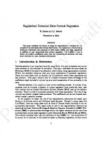
The variable selection property is clearly shown graphically in Figure 1, reproduced from Hastie et al. [2008], when considering two parameter estimates, with the LASSO (black) and ridge (red). The estimator loss functions are shown as ellipses. Figure 1: Differences Between the LASSO and Ridge Regressions 7.5

5.0

y

^ β

ar

β2

2.5

in

0.0

-2.5

0.0

2.5

5.0

β1

m

-2.5

eli

The point of tangency are the estimates for each technique. The LASSO shrinks β1 ˆ Fu to 0, whereas the ridge regression approaches it. The OLS estimator is given as β. and Knight [2000] show that under certain regularity conditions, the estimates of the coefficients are consistent and that these will have the same limiting distribution as the OLS estimates.

2.2

The Skew Normal Distribution

Pr

The skew-normal distribution (SN) has been applied to applications in several fields since the it was introduced in the modern era by Azzalini [1985] and [1986] following Del Helguero [1908]. The standard form of the distribution has the probability density function

3

f (y) = 2φ (y) Φ (λy) ; −∞ < λ < ∞, −∞ < y < ∞,

(3)

Dr af t

with λ controlling the degree of skewness and where φ and Φ are the standard normal probability density and distribution functions respectively. The case λ = 0 leads to a standard normal distribution. Azzalini [1985] and [1986] show that the SN distribution may be thought of as the convolution of a normally distributed variable and an independently distributed normal variable which has a mean of zero and which is truncated from below at zero. This is generalized in Arnold & Beaver [2000] and Adcock & Shutes [2001] where the truncated normal variable has a mean of τ , which may take any real value. Using what is normally referred to as the central parametrization1 , the probability density function of the extended skew-normal (ESN) distribution is p 1 y−µ y−µ f (y) = Φ τ 1 + λ2 + λ . (4) φ ωΦ (τ ) ω ω

−

n X

y

For a linear regression model µ = xT β. Using this notation, the objective function to be minimized for a random sample of size n from the distribution at Equation 4 is log f (yi ) + ν || β ||1 .

i=1

(5)

log f (yi ) + ν1 || β ||1 +ν2 | λ | +ν3 | τ | .

(6)

in

−

n X

ar

Under the ESN distribution, it is also possible to shrink estimates of the parameters λ and τ , which control skewness and other higher moments, using a different shrinkage parameter for each case. The objective function to be minimized is

i=1

eli

m

The number of applications of the LASSO in conjunction with the SN distribution is limited. Wu et al. [2012] consider the variable selection problem for the SN distribution, for which τ = 0. The skewness parameter λ is estimated but is then treated as fixed and omitted from the SN-LASSO; that is, Wu et al minimize the objective function at ˆ The penalized likelihood approach used both in Wu and (5) using a fixed value of λ. in this paper is found in Fan and Li [2001]. To the best of our knowledge there are no applications of the LASSO with the ESN distribution.

2.3

Estimation with Constrained Maximum Likelihood

Pr

The estimation procedure maximizes the value of the objective function at 5, with a grid of values for the penalty parameter ν. The value of the penalty parameter for ESN-LASSO is selected using a cross-validation procedure. The estimation of ν uses 10-fold cross-validation over an identical grid of ν parameter values. The mean squared cross validation (prediction) errors are calculated using the hold-out sample of each cross 1

A different parameterization is given in Adcock and Shutes [2001]. This form of ESN distribution is not considered in this paper.

4

Dr af t

validating sample, with the ν selected by the Min+1 S.E. rule suggested in Hastie et al. [2008], where Min indicates the estimated value of the nuisance parameter that minimizes the mean squared errors in the cross validation and where Min+1S.E. indicates the estimated value of the penalty parameter that has an mean squared error within 1 standard deviation of the minimum value2 .

Pr

eli

m

in

ar

y

In the following sections, results of the estimation procedures are generally presented graphically using the estimated penalty parameter with the estimated penalized parameters presented as a proportion of the unconstrained maximum likelihood estimate, taking the sign of the unconstrained maximum likelihood estimators (MLEs) into account. All estimations are performed using R Core Team [2016] and the packages bbmle (Bolker and Team [2016]), glmnet (Friedman et al. [2010]) and sn (Azzalini [2015]). The results for other data are also estimated using glmnet (Friedman et al. [2010]). The ridge regressions are performed using glmnet with the α = 0 rather than 1 as in the case of the LASSO. The stepwise algorithm is the method in base R. This minimises the AIC (Akaike [1974]).

2 Alternative approaches to estimation are available, such as BIC minimisation or cross-validation based on (minus) the log likelihood function as suggested in St¨ adler et al. [2010], although these are not used in this paper.

5

3

Properties of the ESN LASSO Using Simulated Data

3.1

Dr af t

This section presented the results of applying the ESN-LASSO to a number of simulated data sets, the purpose of which is to demonstrate the method in operation.

Simulation Setup

Results

in

3.2

ar

y

The results reported in this section are based on two linear regression models, referred to below as Model-I and Model-II, with residuals that are independently and identically distributed as extended skew-normal variates with parameters defined in Equation ?? set as follows: µ = 0, σ = 1, λ = −4 and τ = −3 for Model I and with µ = 0, σ = 1, λ = 1 and τ = 1 for Model II . Models-I and -II are both based on ten independent variables. These are randomly generated N(0,1) variates. Fifty different sets of data are used for each model to demonstrate the properties of the LASSO estimation procedure. The simulated data sets are based on 10,000, 1,000 and 100 observations, giving a total of 300 data sets or 6 sets each with 50 replications. In each replication the values of the independent variables are the same. In Model-I the regressions coefficients are set as follows: β1 = −3, β2 = −5, β3 = 0.5 and β5 = 2. The other six regression coefficients are set to zero. In Model-II the coefficients are β1 , β2 = -1, β3 , β5 = 1 , with the other six coefficients set to zero as in Model-I. For this demonstration, ten independent variables are used to reflect the analysis of the diabetes data in Section 4, which also has 10 independent variables. The two skewness parameters are selected to generate residuals that exhibit a significant degree of asymmetry, although by design Model II has less skewness, with γ = τ = 1.

eli

m

Simulation results are presented in detail for N = 10, 000, with corresponding results for N = 1, 000 and 100 reported in the appendix. The figures in this section report the median values of the regression model parameters taken over the 50 replications of each of the model sets. To illustrate the effect of increasing the value of the LASSO penalty ν these are shown as proportions of the unrestricted MLEs, taking the sign into account. The horizontal axis in each figure is log ν rather than ν. The first value on the log(ν) axis represents the unconstrained estimates. Figure 2 shows the impact of increasing the LASSO penalty ν on the values of the estimated regression coefficients for model-I. In general, the coefficients which are non-zero in the model specification (that is, β1,2,3,5 ) remain close the their unrestricted MLE estimates, whereas the estimated values of the remaining six model parameters show a decline towards zero.

Pr

Table 1 has six horizontal panels. Panels 1 through 4 show the medians of the estimated values of the four non-zero model coefficients, β1,2,3,5 , for Model-I at five selected values of log ν. Also shown in each panel of the table are estimated 5%, 25%, 75% and 95% values computed non-parametrically using results from the 50 replications. As these table entries show the estimated coefficients are stable around the unconstrained

6

Dr af t

Figure 2: Median LASSO Regression Coefficients (β) of Variables by ν (N=10000) for Model I 1

Sign(βESN)βi/βESN

0

β1

β6

β2(dotted)

β7(dashed)

β3

β8

β4

β9(dashed)

β5

β10(dashed)

−2

2

ν

4

6

ar

0

y

−1

in

Figure 3: Median Skewness Parameter Estimates of Simulation Data Model I (N=10000)

−0.3

−0.6

Pr

eli

Sign(γESN)γi/γESN and Sign(τESN)τi/τESN

m

0.0

−0.9

γ 0

τ 2

ν

7

4

6

Dr af t

Figure 4: Median LASSO Regression Coefficients (β) of Variables by ν (N=10000) for Model II 1


0

β1

β6

β2(dotted)

β7(dashed)

β3

β8

β4

β9(dashed)

β5

β10(dashed)

−2

2

ν

4

6

ar

0

y

−1

in

Figure 5: Median Skewness Parameter Estimates of Simulation Data Model II (N=10000)

−0.3

−0.6

Pr

eli


m

0.0

−0.9

γ 0

τ 2

ν

8

4

6

4 -1.0000 -0.9998 -0.9998 -0.9998 -0.9996 -1.0000 -0.9999 -0.9999 -0.9998 -0.9998 0.9980 0.9986 0.9986 0.9988 1.0001 0.9993 0.9996 0.9997 0.9997 1.0000 -0.5362 -0.3115 0.0000 113.1959 -0.0002 -0.0001 -0.0000 -0.0000 0.0000

y

2 -1.0000 -1.0000 -1.0000 -1.0000 -0.9999 -1.0001 -1.0000 -1.0000 -1.0000 -0.9999 0.9993 0.9997 0.9998 0.9999 1.0002 0.9999 0.9999 1.0000 1.0000 1.0001 -0.7409 -0.4467 0.0001 153.3652 -0.4985 -0.4123 -0.1341 -0.0000 0.3635

in

eli

Pr

1 -1.0000 -1.0000 -1.0000 -1.0000 -0.9999 -1.0001 -1.0000 -1.0000 -1.0000 -1.0000 0.9997 0.9999 0.9999 1.0000 1.0000 1.0000 1.0000 1.0000 1.0000 1.0001 -1.0000 -0.8796 0.0033 195.3219 -1.0000 -1.0000 -0.6927 -0.0000 0.6462

ar

0 -1.0000 -1.0000 -1.0000 -1.0000 -1.0000 -1.0000 -1.0000 -1.0000 -1.0000 -1.0000 0.9999 1.0000 1.0000 1.0000 1.0000 1.0000 1.0000 1.0000 1.0000 1.0000 -1.0000 -1.0000 0.9994 195.9941 -1.0000 -1.0000 -1.0000 -0.2851 1.0000

m

β1 β1 β1 β1 β1 β2 β2 β2 β2 β2 β3 β3 β3 β3 β3 β5 β5 β5 β5 β5 γ γ γ γ τ τ τ τ τ

ν= Q05 Q25 Q50 Q75 Q95 Q05 Q25 Q50 Q75 Q95 Q05 Q25 Q50 Q75 Q95 Q05 Q25 Q50 Q75 Q95 Q25 Q50 Q75 Q95 Q05 Q25 Q50 Q75 Q95

Dr af t

MLE. The final two rows present the proportions of the MLE estimates for λ and τ . Similar results for the regression coefficients in Model-II are shown in Figure 4 and panels 1 through 4 of Table 2. Figures 3 and 5 show the corresponding estimates for the skewness and truncation parameters, λ and τ , for Models-I and -II respectively. These are shrunk in the same manner to those for the estimated regression coefficients; the magnitude of estimates declines to zero as ν increases. The contraction of the λ andτ parameters are consistent with the convergence of the ESN to the Gaussian distribution as the constraint binds tighter. The corresponding results for 1,000 and 100 observations are shown in the appendix. 6 -0.9990 -0.9986 -0.9984 -0.9983 -0.9980 -0.9994 -0.9991 -0.9990 -0.9989 -0.9986 0.9875 0.9898 0.9907 0.9915 0.9941 0.9966 0.9975 0.9976 0.9979 0.9988 -0.0000 -0.0000 0.0000 0.0010 -0.0000 -0.0000 -0.0000 -0.0000 0.0000

Table 1: Table Showing Inter-Quantile Range for Estimates of β at selected values of ν (N=10000)

9

m eli

Dr af t

2 -0.9996 -0.9994 -0.9994 -0.9994 -0.9993 -0.9995 -0.9994 -0.9994 -0.9994 -0.9993 0.9993 0.9994 0.9994 0.9994 0.9995 0.9993 0.9994 0.9994 0.9994 0.9997 -0.0001 -0.0000 -0.0000 0.8571 0.9619 -0.0005 -0.0000 -0.0000 -0.0000 0.0004

4 -0.9965 -0.9960 -0.9957 -0.9955 -0.9948 -0.9965 -0.9959 -0.9956 -0.9954 -0.9948 0.9947 0.9955 0.9957 0.9958 0.9963 0.9950 0.9955 0.9957 0.9960 0.9969 -0.0009 -0.0001 -0.0000 0.0000 0.0000 -0.0000 -0.0000 -0.0000 -0.0000 0.0000

y

1 -0.9999 -0.9998 -0.9998 -0.9998 -0.9997 -0.9999 -0.9998 -0.9998 -0.9998 -0.9997 0.9997 0.9998 0.9998 0.9998 0.9999 0.9997 0.9998 0.9998 0.9998 0.9999 -0.0008 -0.0004 -0.0001 0.8737 0.9831 -0.0019 -0.0000 -0.0000 -0.0000 0.5985

ar

0 -1.0000 -0.9999 -0.9999 -0.9999 -0.9998 -1.0000 -0.9999 -0.9999 -0.9999 -0.9999 0.9998 0.9999 0.9999 0.9999 1.0000 0.9998 0.9999 0.9999 0.9999 1.0000 -0.9998 -0.9992 -0.1828 0.9503 0.9998 -1.0000 -0.9999 -0.6146 -0.0000 0.9977

in

β1 β1 β1 β1 β1 β2 β2 β2 β2 β2 β3 β3 β3 β3 β3 β5 β5 β5 β5 β5 γ γ γ γ γ τ τ τ τ τ

ν= Q05 Q25 Q50 Q75 Q95 Q05 Q25 Q50 Q75 Q95 Q05 Q25 Q50 Q75 Q95 Q05 Q25 Q50 Q75 Q95 Q05 Q25 Q50 Q75 Q95 Q05 Q25 Q50 Q75 Q95

6 -0.9732 -0.9702 -0.9690 -0.9675 -0.9662 -0.9733 -0.9704 -0.9685 -0.9674 -0.9651 0.9657 0.9677 0.9691 0.9707 0.9726 0.9667 0.9680 0.9690 0.9705 0.9727 -0.0004 -0.0001 -0.0000 0.0000 0.0000 -0.0000 -0.0000 -0.0000 -0.0000 0.0000

Pr

Table 2: Table Showing Inter-Quantile Range for Unit Estimates of β at selected values of ν (N=10000)

10

4

Bicycle Hire

Dr af t

This data set was acquired from the Capital Bikeshare System in Washington DC. The data set is based on 17379 hourly observations with the aggregation being created by Fanaee-T and Gama [2013]. This data reports the determinants of bicycle hire based on three sets of variables. These are (i) season of the year, (ii) whether the day is a public holiday or work day and (iii) weather. The six weather variables are wind speed, humidity, temperature (normalized to 41 degrees) and three binary general weather situation variables, referred to in the data set as clear, light rain and snow. The seasons are defined as the four quarters (months by quarter and observations in each month are given in Table 3). In the analysis these are dummy variables, with Q4 (September to early December) being the base observations per variable. The dependent variable in the regressions is logarithm of the number of hires. This is a large and interesting data set that to the best of our knowledge has not been studied in depth by statisticians previously. The summary statistics are presented in Table 5. All the variables exhibit high levels of skewness and excess kurtosis. The diurnal distribution of hires is shown in Table 4. Mar 949 524 0 0

Apr 0 1437 0 0

May 0 1488 0 0

June 0 960 480 0

Jul 0 0 1488 0

Aug 0 0 1475 0

Sep 0 0 1053 384

y

1 2 3 4

Feb 1341 0 0 0

ar

Q Q Q Q

Jan 1429 0 0 0

Oct 0 0 0 1451

Nov 0 0 0 1437

Dec 523 0 0 960

in

Table 3: Classification of Months By Quarter

m

Time of Day [0,6] (6,12] (12,18] (18,24]

Median(Number of Rentals) 16.00 204.00 281.00 155.00

Table 4: Rentals by 6 hour Period

Pr

eli

The paths of the coefficients of the independent variables with increasing penalty are shown in Figures 7 and 8. The estimated values,, based on 10 fold cross validation, of λ and τ are -2.984 and 0.0001 respectively. The ESN LASSO gives a more parsimonious model, at the expense of the R2 , though it must be remembered that the distributional parameters are not fully accounted for using the residuals. One thousand simulations based upon the estimated parameters in the ESN regression and the R2 associated with these. The range of the measures was 0.161 to 0.20, putting the ESN models’ R2 below that of the Gaussian approaches. It is noticeable that the intercepts of the ESN models are both higher than those of the Gaussian distribution; the mean of the distribution

11

Q1

Q2

Q3

Q4

1000 ● ● ●●

●

● ● ● ● ● ● ● ● ● ●● ● ● ●●

●

●

750

●● ● ● ● ●● ●● ●

●●●

●

● ●

Hires

●

500

● ● ● ● ● ● ● ● ● ● ● ● ● ● ● ● ● ● ● ● ● ● ● ● ● ●

250

0

● ● ● ● ● ● ● ● ● ● ● ● ● ● ● ● ● ● ● ● ● ● ● ● ●

0

● ● ● ● ● ● ● ● ● ● ● ● ● ● ● ● ● ● ● ● ● ●

● ● ● ● ● ● ● ● ● ● ● ● ● ● ● ● ● ● ●

● ● ● ● ● ● ● ● ● ● ● ● ● ● ● ● ● ● ● ● ● ●● ● ● ● ●● ● ● ● ● ● ● ● ● ●● ●● ●● ● ● ● ● ● ●● ● ● ● ● ●

5

● ● ● ● ● ● ● ● ● ● ● ● ● ● ● ● ● ● ● ● ● ● ● ● ● ● ● ● ● ● ● ● ● ● ● ● ●

● ● ● ● ● ● ● ● ● ● ● ● ● ● ● ● ● ● ● ● ● ● ● ● ● ● ● ● ● ●

● ● ●

● ●

●

● ● ● ● ●● ●

●

●

● ●

●

● ● ●

●

●● ●● ● ● ● ●● ● ●● ●● ● ● ● ● ●● ● ● ●● ● ● ● ●● ● ● ● ● ● ● ● ● ● ●● ● ● ● ● ● ● ●● ● ● ● ● ● ● ● ● ● ● ●● ● ● ● ●● ● ● ● ● ● ● ●● ● ●● ● ● ● ●● ● ● ● ● ● ●● ● ● ● ● ● ●● ● ● ● ● ● ● ● ● ● ● ● ●● ● ● ● ● ● ● ● ● ● ●● ● ● ● ● ●● ● ● ● ●

●

● ● ● ● ● ● ● ● ● ● ● ● ● ● ● ● ● ● ● ● ● ● ● ● ● ● ● ● ● ● ● ● ● ● ● ● ● ● ● ● ● ● ● ● ● ●

●● ● ●●● ●● ●● ● ● ● ●●●● ●● ●● ●●● ● ● ●● ● ●●●● ● ● ● ●●● ●● ●● ● ● ●● ● ●● ● ● ● ● ●● ● ●● ● ● ● ● ●● ●● ●● ●● ● ● ●● ● ●● ● ● ● ● ● ● ● ● ●● ●● ●● ● ●●● ●● ● ● ● ● ● ● ● ●● ●● ● ●● ● ● ● ● ● ●● ● ●● ● ● ● ●●● ●● ● ● ●●● ● ● ● ● ●● ●● ● ● ●● ● ● ● ●● ● ● ● ● ● ● ● ● ● ●● ● ● ● ● ● ● ●● ●● ● ● ● ● ● ● ●● ● ● ●● ●● ● ●● ● ●● ● ● ● ● ● ● ● ●●● ●● ● ● ● ● ● ● ●● ● ● ● ● ● ● ● ● ● ● ● ● ●● ●● ● ●● ● ● ● ●● ● ● ●●● ● ● ●●● ● ●● ● ● ● ● ● ●● ●●● ●

10

●

● ● ●● ● ● ●● ● ● ● ● ● ● ● ● ● ● ● ● ● ● ● ● ● ● ● ● ● ● ● ● ● ● ● ● ● ● ● ● ● ● ● ● ● ● ● ● ● ● ● ● ● ● ● ● ● ● ● ● ● ● ● ● ● ● ● ● ● ● ● ● ● ●

● ● ● ● ● ● ● ● ● ● ● ● ● ● ● ● ● ● ● ● ● ● ● ● ● ● ● ● ● ● ● ● ● ● ● ● ● ● ● ● ● ● ● ● ● ● ● ● ● ● ● ● ● ● ● ● ● ● ● ● ● ● ● ● ● ● ● ● ● ● ● ●

● ● ● ● ● ● ● ● ● ● ● ● ● ● ● ● ● ● ● ● ● ● ● ●

● ●● ●● ● ● ● ●

● ●● ● ● ●● ● ● ● ● ●● ● ● ● ● ●●● ●●● ●●●● ● ● ● ● ● ● ● ●●● ● ● ●●● ● ●● ●● ●● ● ● ●●● ● ●●●● ● ● ●● ● ● ● ● ● ●● ● ● ● ● ●●● ● ●● ●● ●●● ●● ● ● ● ●●● ●● ● ● ●● ●● ● ● ● ●● ● ● ● ● ● ● ● ● ●● ● ●● ● ● ●● ● ● ● ● ● ● ● ●● ● ● ●● ● ● ● ● ● ● ● ● ● ● ● ●● ● ●● ● ●● ●● ● ● ● ● ● ● ● ●● ●● ● ●● ● ● ● ● ●● ● ● ● ● ● ●● ● ● ● ●● ●● ● ● ● ● ● ● ●● ●● ● ●● ● ● ● ● ●● ● ● ●● ● ● ● ● ●●● ● ● ● ●● ●● ● ● ● ●● ● ● ● ● ●●● ● ●● ● ● ●● ● ● ●●● ● ● ● ● ●● ● ● ●● ●● ●●

15

● ● ● ● ● ● ● ● ● ● ● ● ● ● ● ● ● ● ● ● ● ● ● ● ● ● ● ● ● ● ● ● ● ● ● ● ● ● ● ● ● ● ● ● ● ● ● ● ●

20

● ● ●● ● ● ● ● ● ● ● ● ●● ● ● ●● ● ● ●● ● ● ● ● ● ●● ● ● ● ● ● ● ● ● ● ● ●● ● ● ● ● ● ●● ● ● ● ● ● ● ●● ● ● ●● ● ● ● ● ● ● ● ●● ● ● ● ●

● ● ● ● ● ● ● ● ● ● ● ● ● ● ● ● ● ● ● ● ● ● ● ● ● ● ● ● ● ● ● ● ● ● ● ● ● ● ● ● ●

0

● ● ● ● ● ● ● ● ● ● ● ● ● ● ● ● ● ● ● ● ● ● ● ● ● ● ● ● ● ● ● ●

● ● ● ● ● ● ● ● ● ● ● ● ● ● ● ● ● ● ● ● ● ● ●

● ● ● ● ● ● ● ● ● ● ● ● ● ● ● ● ● ● ● ● ● ● ● ● ● ● ● ● ● ● ● ● ● ● ● ● ● ●● ● ● ● ● ● ● ● ● ● ● ● ● ● ● ● ● ●● ● ● ● ● ● ● ● ● ●● ●● ● ● ●● ● ● ● ● ●● ●● ●●

5

● ● ● ● ● ● ● ● ● ● ● ● ● ● ● ● ● ● ● ● ● ● ● ● ● ● ● ● ● ● ●● ● ● ● ●● ●● ● ●● ● ● ● ● ●● ● ● ● ● ● ● ●● ● ●● ● ● ●● ●● ● ● ●● ● ●● ● ● ● ● ● ●● ● ● ●● ● ● ● ●● ● ●● ● ●● ● ● ● ● ● ●● ● ● ●● ● ● ● ● ●● ● ● ●● ● ●● ●● ● ● ● ●● ● ●● ● ●● ●● ● ● ●● ● ● ● ● ●● ●● ●● ● ● ● ● ●● ● ● ●● ● ● ● ●● ● ●● ● ● ● ● ●● ● ● ● ● ● ● ● ● ●● ● ● ● ● ● ●● ● ● ● ● ● ●● ● ● ● ● ● ● ● ●● ● ●

●

● ● ● ● ● ● ● ● ● ● ● ● ● ●● ●● ●● ●● ● ●● ● ●● ● ● ●● ●●● ●●● ● ●●● ● ● ●● ● ● ● ● ●●● ● ● ● ●●● ● ● ●● ● ●● ● ● ● ● ● ●● ● ●● ● ●●● ● ● ●●● ● ● ● ● ●● ● ● ● ●●● ● ●● ● ●● ●● ● ● ●● ●● ● ● ●● ● ● ●● ●● ● ● ● ●● ● ● ● ● ● ●● ● ● ●● ● ● ● ● ● ● ●● ●● ● ● ● ● ● ●● ● ● ● ● ●●● ● ● ● ● ● ●● ● ● ● ● ● ●● ●● ● ●● ● ● ● ● ● ● ●● ●● ● ● ● ● ●● ●● ● ● ● ● ● ●● ●● ● ●● ● ●●● ● ● ● ●● ●● ● ● ●●● ● ●● ● ● ●● ●● ●● ●

10

● ● ● ●● ●● ● ● ●● ●● ● ● ●● ● ● ●● ●● ● ●● ● ●● ●● ● ● ● ●●● ● ●●● ● ● ● ●● ● ●● ● ● ●●● ●●● ● ● ●● ●●● ● ●●● ●● ●● ● ●●● ● ● ● ● ●●● ●● ●● ● ●● ● ● ● ● ● ●● ● ●● ● ● ●● ● ● ●●● ● ● ● ●● ●● ●● ●● ● ●● ● ● ● ● ● ●● ●● ● ● ● ● ● ● ●● ●● ● ● ●● ● ● ● ●●● ● ● ● ●● ●● ● ● ●● ●● ● ● ● ● ●● ●● ● ● ● ● ● ● ●● ● ●● ● ● ● ● ● ● ● ●● ● ● ●● ● ● ●● ● ● ●● ● ●● ● ●● ●● ● ● ● ● ● ●● ●● ● ● ● ● ● ●● ● ● ● ●● ●● ● ● ●● ● ●●● ● ●● ● ●● ● ● ● ● ●● ● ● ● ● ● ●●● ● ● ●● ● ●● ●● ●● ● ●● ● ● ●

● ● ● ● ● ● ● ● ● ● ● ● ●

● ● ● ● ● ● ● ● ● ● ● ● ● ● ●

●● ● ●● ● ●● ● ●● ● ● ● ● ● ● ● ●● ● ● ●● ● ● ●● ● ● ●● ● ● ● ● ● ●● ● ● ● ● ● ●● ● ● ● ●● ● ● ● ●● ● ●● ● ● ●● ● ● ● ●● ● ●● ● ●● ● ● ● ● ● ● ● ●● ● ● ● ● ● ● ●● ● ● ● ● ●● ● ● ● ● ● ● ● ● ●● ● ● ● ●● ● ● ● ● ● ● ●● ● ● ●● ● ● ● ● ●● ●● ● ●● ● ● ● ● ● ●● ● ● ● ●● ●● ● ● ● ● ● ● ●●

● ● ● ● ● ● ● ● ● ● ● ● ● ● ● ● ● ● ● ● ● ● ● ● ● ● ● ● ● ● ● ● ● ● ●

● ● ● ● ● ● ● ● ● ● ● ● ● ● ● ● ● ● ● ● ● ● ● ● ● ● ● ● ● ● ● ● ● ● ● ● ● ● ● ● ● ● ● ● ● ● ● ● ● ● ● ● ● ● ● ● ● ● ● ● ● ● ● ● ● ● ● ● ● ● ● ● ● ● ● ● ● ● ● ● ● ● ● ● ● ● ● ● ● ● ● ● ● ● ● ● ● ● ● ● ● ● ● ● ● ● ● ●

●● ● ● ●

●● ●● ● ● ●

15

●

● ● ● ● ● ● ● ● ● ● ● ● ● ● ● ● ● ● ● ● ● ● ● ● ● ● ● ● ● ● ● ● ● ● ● ● ● ● ● ● ● ● ● ● ● ● ● ● ● ● ● ● ● ● ● ● ● ● ● ● ● ● ● ● ● ● ● ● ● ● ● ● ● ● ● ● ● ● ● ● ● ● ● ● ● ● ● ● ● ● ● ●

● ● ●● ●● ●

● ● ● ● ● ● ● ● ● ● ● ● ● ● ● ● ● ● ● ● ● ● ● ● ● ● ● ● ● ● ● ● ● ● ● ● ● ● ● ● ● ● ● ● ● ● ● ● ● ● ● ● ● ● ● ● ● ● ● ● ● ● ● ● ● ● ● ● ● ● ● ● ● ● ● ● ● ● ● ● ●

● ● ● ● ● ● ●● ● ● ● ● ● ● ● ● ● ●● ● ● ● ● ● ● ● ● ●● ● ● ● ● ● ● ● ●● ● ● ●● ● ● ● ● ●● ● ●● ● ●● ● ● ● ● ● ● ● ●● ● ● ● ● ● ● ● ● ● ● ●● ● ● ●● ● ● ●● ● ● ● ● ● ● ● ● ●● ● ● ● ●● ● ● ●● ● ● ● ● ● ●● ● ● ● ● ● ● ● ● ● ● ●● ● ● ● ●● ● ● ● ●● ●● ●

● ● ● ● ● ● ● ● ● ● ● ● ● ● ● ● ● ● ● ● ● ● ● ● ● ● ● ● ● ● ● ● ● ● ● ● ● ● ● ● ● ● ● ● ● ● ● ● ● ●

20

● ● ● ● ● ● ● ● ● ● ● ● ● ● ● ● ● ● ● ● ● ● ● ● ● ● ● ● ● ● ● ● ● ● ● ● ● ● ● ● ● ● ● ●

● ● ● ● ● ● ● ● ● ● ● ● ● ● ● ● ● ● ● ● ● ● ● ● ● ● ● ●

● ● ● ● ● ● ● ● ● ● ● ● ● ● ● ● ● ● ● ● ● ● ● ● ● ● ● ● ● ● ● ● ● ●

● ● ● ● ● ● ● ● ● ● ● ● ● ● ● ● ● ● ● ● ● ● ● ● ● ● ●

● ● ● ● ● ● ● ● ● ● ● ● ● ● ● ● ● ● ● ●● ●● ● ● ● ● ● ● ● ● ●● ● ● ● ●● ●●

0

5

● ● ● ● ● ● ● ● ● ● ● ● ● ● ● ● ● ●

● ● ● ● ● ● ● ● ● ● ● ● ● ● ● ● ● ● ● ● ● ● ● ● ● ● ● ● ● ● ● ● ● ● ● ● ● ●● ● ●● ● ● ●● ● ●● ● ● ● ● ● ● ● ●● ● ● ● ●● ●● ● ● ●● ● ● ●● ● ●● ● ● ● ● ● ● ●● ● ● ● ●● ● ● ● ● ●● ● ● ●● ●● ● ● ● ●● ●● ● ● ● ● ●● ● ● ● ● ● ● ● ●● ● ● ● ● ● ● ● ● ● ● ●● ● ● ● ● ● ●● ●● ● ● ● ● ●● ● ● ● ● ● ●● ● ● ● ● ●● ● ● ● ●● ● ● ● ● ● ● ● ● ● ● ● ● ● ●

●

● ● ● ● ●● ● ●● ● ●● ● ● ●

● ● ● ● ● ● ● ● ● ● ● ● ● ● ● ● ● ● ● ● ● ● ● ● ● ● ● ● ● ● ● ● ● ● ● ● ● ● ● ● ● ● ● ● ● ● ● ● ● ● ● ● ● ● ● ● ● ● ● ● ● ● ●

● ● ● ● ● ● ●● ● ●● ● ● ● ●● ● ● ● ● ● ● ● ●● ● ● ● ●● ● ●● ●● ● ● ● ● ● ●● ● ● ● ●● ● ● ● ● ● ●● ● ●● ● ●● ● ● ● ●● ● ● ● ● ●● ● ● ● ● ● ● ● ● ● ● ● ● ●● ● ●● ● ● ● ● ● ● ● ● ●● ● ● ● ● ● ●● ● ● ●● ● ● ● ● ● ● ● ● ● ●● ● ●● ● ● ●● ● ● ● ● ●● ● ● ● ● ● ● ●● ● ● ●● ● ● ●● ●● ● ● ● ● ●

10

● ● ● ● ● ● ● ● ● ● ● ● ● ● ● ● ● ● ● ● ● ● ● ● ● ● ● ● ● ● ● ● ● ● ● ● ● ● ● ● ● ● ● ● ● ● ● ● ● ● ● ● ● ● ● ● ● ● ● ● ● ● ● ● ● ● ● ● ● ● ● ● ● ● ● ● ● ● ●

● ● ● ● ● ● ● ● ● ● ● ● ● ● ● ● ● ● ● ● ● ●

●● ● ● ●● ●● ●● ●●

● ● ● ● ● ● ● ● ● ●

Dr af t

●

● ● ● ● ● ● ● ● ● ● ● ● ● ● ● ● ● ● ● ● ● ● ● ● ● ● ● ● ● ● ● ● ● ● ● ● ● ● ● ● ● ● ● ● ● ● ● ● ● ● ● ● ● ● ● ● ● ● ● ● ● ● ● ● ● ● ● ● ● ●

● ● ● ● ● ● ● ● ● ● ● ● ● ● ● ● ● ● ● ● ● ● ● ●● ● ● ● ● ● ● ● ● ● ● ● ● ● ● ●●● ● ● ● ● ● ●● ● ● ●● ● ● ● ● ●● ●●● ● ● ● ● ● ● ●● ●●● ● ● ● ● ●● ● ● ● ● ● ● ●● ● ● ●●● ● ● ● ● ● ● ●● ● ● ●● ● ● ●●●● ● ● ●● ● ●●●● ● ● ● ● ● ● ● ● ● ● ● ● ● ●● ● ●● ●●● ● ● ●● ● ● ●●●●● ● ● ●● ● ● ●●● ● ●● ●●● ● ● ●● ● ● ●●●● ●● ● ● ●●● ● ● ● ● ● ● ●●● ● ● ●●● ● ●● ● ● ● ● ● ●●● ● ●● ●● ●● ●● ● ● ● ●● ● ● ●● ●● ●● ● ● ●●● ● ● ● ● ● ● ● ● ● ●●●●● ● ● ●●● ●● ● ●● ● ● ● ● ●● ●● ● ●●● ● ● ● ● ● ● ● ● ● ● ● ● ● ●●● ● ●● ●● ● ● ●● ● ● ●● ● ● ● ● ●●● ●●● ● ● ● ●●● ● ● ● ●● ● ● ● ● ● ● ● ●●● ●● ●● ● ● ●● ●● ●● ● ● ● ●● ●● ●● ●● ● ● ●● ●● ●● ●● ● ● ●● ● ●● ● ●● ●● ●● ●● ●● ●● ●● ● ● ● ● ●● ● ● ● ● ●● ●● ●● ● ● ● ● ●●● ● ● ● ● ● ●● ● ● ● ●●● ●● ●● ● ● ● ● ● ● ● ●● ●● ● ●● ● ● ●● ●● ● ● ● ●●● ●● ●● ● ●● ●● ● ● ● ● ● ● ● ●●●● ● ●

●● ●● ● ● ●● ● ● ● ● ●● ● ● ● ● ●● ● ●● ●● ● ●● ●● ● ● ●● ● ●● ● ●● ● ● ● ●● ● ● ● ●● ● ● ● ●● ●● ● ● ● ● ●● ● ● ● ●● ● ●● ●● ● ●● ●● ● ●● ● ● ● ● ● ● ●● ● ●● ● ● ● ● ● ● ●● ● ● ●● ● ●● ● ● ● ●● ● ● ● ● ●● ●● ● ● ●● ● ● ● ●● ● ● ● ● ●● ● ● ● ●● ● ●● ● ● ● ●● ● ●● ●● ● ●● ● ●● ●● ● ●●

● ● ● ● ● ●

●

●

● ● ● ● ● ● ● ● ● ● ● ● ● ● ● ● ● ● ● ● ● ● ● ● ● ● ● ● ● ● ● ● ● ● ● ● ● ● ● ● ● ● ● ● ● ● ● ● ● ● ● ● ● ● ● ● ● ● ● ● ● ● ●

● ● ● ● ● ● ● ● ● ● ● ● ● ● ● ● ● ● ● ● ● ● ● ● ● ● ● ● ● ● ● ● ● ● ● ● ● ● ● ● ● ● ● ● ● ● ● ● ● ● ● ●● ● ●● ● ● ●● ● ●● ●

20

●

● ●

● ● ●● ●

● ● ● ●

●

● ● ● ● ● ● ● ● ● ● ● ● ● ● ● ● ● ● ● ● ● ● ● ● ● ● ● ● ● ● ● ● ● ● ● ● ● ● ● ● ● ● ● ● ● ● ● ● ● ● ● ● ● ● ● ● ● ● ● ● ● ● ● ●●● ● ● ●● ●● ● ● ●● ● ● ● ● ● ● ● ●●

15

●

● ● ● ● ● ● ● ● ● ● ● ● ● ● ● ● ● ● ● ● ●

● ● ●

●

● ● ● ● ● ● ● ● ● ● ● ● ● ● ● ● ● ● ● ● ● ● ● ● ● ● ● ● ● ● ● ● ● ● ● ● ● ● ● ● ● ● ● ● ● ● ●

●

● ● ● ● ● ● ● ● ● ● ● ● ● ● ● ● ● ● ● ● ● ● ● ● ● ● ● ● ● ● ● ●

● ● ● ● ● ● ● ● ● ● ● ● ● ● ● ● ● ● ● ● ● ● ● ● ● ● ● ● ● ● ● ● ● ●

● ● ● ● ● ● ● ● ● ● ● ● ● ● ● ● ● ● ● ● ● ● ● ● ●

0

●

● ● ● ● ● ● ● ● ● ● ● ● ● ● ● ● ● ● ● ● ● ● ● ● ● ●● ● ● ● ● ● ● ● ●● ●●

● ● ● ● ● ● ● ● ● ● ● ● ● ● ● ● ● ● ● ● ● ● ● ● ● ● ● ● ● ● ● ● ● ● ● ● ● ● ● ● ● ● ●

5

● ● ● ● ● ● ● ● ●● ●● ●● ● ●● ● ● ● ●● ● ● ● ● ● ● ●● ● ● ● ● ● ● ●● ● ● ● ● ● ● ● ●● ● ● ● ● ● ● ●● ● ● ● ● ● ●● ● ● ● ● ● ● ● ● ● ● ● ● ● ●● ● ● ● ● ● ● ● ● ● ● ●● ● ● ● ●● ● ● ● ●● ● ● ●● ●● ●● ● ●● ●● ● ● ● ● ● ●● ● ● ● ● ●● ● ● ● ● ● ● ● ● ●● ● ● ● ● ● ●● ● ● ● ● ● ● ●

●

● ● ● ● ● ● ● ● ● ● ● ● ● ● ● ● ● ● ● ● ● ● ● ● ● ● ● ● ● ● ● ● ● ● ● ● ● ● ● ● ● ● ● ● ● ● ● ● ● ● ● ● ● ● ● ● ● ● ● ● ● ● ● ● ● ● ● ● ● ● ● ● ● ●

●● ● ●● ●● ● ● ●

● ●● ● ●●● ● ●●● ●● ● ● ●●● ● ● ●● ● ● ● ●●● ●● ● ●● ● ●● ● ●● ●● ● ●● ● ● ● ● ● ●● ●● ●●● ● ● ●●● ● ●● ● ● ●● ● ●● ● ● ● ● ●● ●● ●● ● ● ● ●●● ● ● ●● ●● ● ● ● ● ● ●● ●● ● ● ● ● ● ● ●● ● ● ● ●● ● ● ●● ● ● ● ● ● ●● ● ● ●● ● ● ● ● ●● ● ● ●● ●● ● ● ● ● ● ● ● ● ● ● ● ●● ●● ● ●● ● ● ● ● ● ● ● ● ● ●● ●● ● ● ● ● ●● ●● ● ● ●● ● ● ● ● ●●● ● ● ● ● ● ● ● ●● ● ●●● ● ●●● ● ●●● ● ● ●● ● ●●●

10

●

● ●●

● ● ●●● ● ● ●●● ● ● ● ● ●● ● ●● ●● ● ●●●● ●●● ●● ● ●●● ● ●●● ● ● ●●●● ●● ● ● ●● ●● ● ●● ● ● ● ● ●●● ●● ● ● ●●● ●● ●● ● ● ● ● ●● ● ●● ● ● ●● ●●● ● ● ● ● ●●●●● ● ● ●●● ●● ● ●● ●● ● ●● ● ● ● ● ●● ● ●●● ●● ● ● ●● ● ● ●● ● ● ●● ●● ● ● ● ● ● ● ● ● ●●●●● ● ● ● ● ● ● ● ● ●● ● ● ● ●● ●● ●●● ● ●● ● ● ● ● ● ●● ● ●● ● ● ●●● ●●● ● ● ●● ● ● ●● ●● ●● ● ● ● ● ● ● ● ● ● ●● ●● ●● ● ●● ● ● ●● ●● ●● ● ● ● ●●● ●● ●● ● ● ● ● ●● ● ●● ● ●● ● ● ● ● ● ● ● ●● ●●● ●● ● ●● ● ● ● ● ● ● ● ● ●● ● ●● ●● ●● ● ● ● ● ●● ● ●● ●● ● ● ● ● ● ● ●● ●● ●● ● ● ●● ●● ●● ● ● ● ●● ●● ● ● ● ●● ● ● ● ●● ●● ● ● ● ● ● ●● ●● ● ●● ● ● ● ● ● ● ● ●●● ●● ● ●● ● ●● ●● ● ● ● ● ● ● ● ● ● ● ● ● ● ● ● ●● ●● ● ● ●● ● ● ● ● ● ●● ●●●● ● ● ● ● ●●● ●● ●● ●● ●●● ● ●● ● ●● ● ● ● ● ● ●● ● ●●● ●● ●● ●● ●● ● ●● ●●● ● ●● ●● ● ● ●

●

●

● ● ● ● ●

●

● ● ● ● ● ● ● ● ● ● ● ● ● ● ● ● ● ● ● ● ● ● ● ● ● ● ● ● ● ● ● ● ● ● ● ● ● ● ● ● ● ● ● ● ● ●

● ● ● ● ● ● ● ● ● ● ● ● ● ● ● ● ● ● ● ● ● ● ● ● ● ● ● ● ● ● ● ● ● ● ● ● ● ● ● ● ● ● ● ● ● ● ● ● ● ● ● ● ● ● ● ● ● ● ● ● ● ● ● ● ● ● ● ● ● ● ● ● ● ● ● ● ● ● ● ● ● ●

●

● ● ● ● ● ● ● ● ● ● ●● ● ● ● ● ● ● ● ● ● ● ● ● ● ● ● ● ● ●● ● ● ●● ● ● ● ● ● ●● ● ● ● ● ● ●● ● ● ● ● ●● ● ● ● ●● ● ● ● ● ● ● ● ● ● ●● ● ● ● ● ● ● ● ● ● ●● ● ● ● ● ● ● ● ● ● ● ● ● ● ●● ● ● ● ● ● ● ●● ● ● ● ●● ● ● ● ● ● ●● ● ● ● ● ● ●● ● ● ● ● ●● ● ● ● ● ● ● ● ● ●● ● ● ● ● ● ●● ● ● ● ● ● ●● ●● ● ● ●● ● ● ● ● ● ● ●● ●●● ● ● ●● ● ● ● ●● ●● ●

15

● ● ● ● ● ● ● ● ● ● ● ● ● ● ● ● ● ● ● ● ● ● ● ● ● ● ● ● ● ● ● ● ● ● ● ● ● ● ● ● ● ● ● ● ● ● ● ● ● ● ● ● ●

● ● ● ● ● ● ● ● ● ● ● ● ● ● ● ● ● ● ● ● ● ● ● ● ● ● ● ● ● ● ● ● ● ● ● ● ● ● ● ● ● ● ● ● ● ● ● ● ●

20

y

Hour of Day

ar

Figure 6: Bicycle Rentals By Hour of the Day

Pr

eli

m

in

is modified by the λ and τ estimates. Further the coefficients under the unconstrained estimation have similar characteristics with respect to significance, though the Working day variable does not bear the same sign. In both cases, the snow variable is the only insignificant variable. As in the case of the diabetes data, the LASSO models both shrink the coefficients for all variables that are selected in the regressions. Indeed, all variables except Ligth rain, Q3 and the intercepts are shrunk in magnitude by using the ESN model and LASSO, both Gaussian and ESN variants. There is significant skewness parameters, both λ andτ , though the τ parameter shrinks towards zero more than the λ parameter.

12

1.0

Work

Dr af t

Temp Wind

0.5

Humidity


Clear

0.0

Light Rain Snow

-0.5

Holiday Q1 Q2

-1.0

Q3

0

2

4

6

8

y

ν

ar

Figure 7: Path of Index Parameters for the Extended Skew Normal LASSO

m

Sign(λ ESN)λ i/λ ESN & Sign(τ

ESN)τ i/τ ESN

-0.25

in

0.00

τ

eli

-0.50

γ

-0.75

Pr

-1.00

0

2

4

6

8

ν

Figure 8: Path of Skewness Parameters λ & τ for the Extended Skew Normal LASSO

13

Snow

Humidity

Holiday

Dr af t Light rain

0.00 0.00 1.00 0.68 0.47 1.00 1.00 -0.79 -1.38 1785.76 1385.98 3171.74

0.00 0.00 1.00 0.66 0.47 1.00 1.00 -0.66 -1.56 1262.13 1771.86 3033.99

0.00 0.00 0.00 0.08 0.27 0.00 1.00 3.06 7.34 27042.50 38973.00 66015.49

0.00 0.00 0.00 0.00 0.01 0.00 1.00 76.09 5788.00 16770735.50 24258872521.25 24275643256.75

0.00 0.48 0.63 0.63 0.19 0.78 1.00 -0.11 -0.83 35.87 494.32 530.19

0.00 0.00 0.00 0.03 0.17 0.00 1.00 5.64 29.79 92072.85 642517.89 734590.74

y

0.02 0.34 0.50 0.50 0.19 0.66 1.00 -0.01 -0.94 0.10 642.45 642.56

Clear

Temp

0.00 0.10 0.19 0.19 0.12 0.25 0.85 0.57 0.59 957.17 252.33 1209.50

Working day

Windspeed

0.00 3.69 4.96 4.54 1.49 5.64 6.88 -0.94 0.17 2538.16 21.97 2560.13

in

ar

Log Cnt Min. 1st Qu. Median Mean Std Dev 3rd Qu. Max. Skewness Excess Kurtosis Skewness JB Kurtosis JB Jarque Bera

Pr

eli

m

Table 5: Summary Statistics for Bicycle Data

14

Dr af t

Table 6: Estimates of the Extended Skew Normal LASSO for Bicycle Data

ar

y

ESN OLS ESN OLS Coef SE LASSO LASSO Ridge Intercept 13.541 1.545 4.760 6.109 4.927 Windspeed 0.146 0.061 0.1740 - 0.511 Temp 2.441 0.063 3.085 1.181 2.833 Working day 0.118 0.0151 - -0.058 Clear -0.121 0.017 -0.120 - -0.191 Light rain -0.267 0.029 -0.025 - -0.208 Snow 0.258 0.539 - 0.731 Humidity -1.282 0.0465 -2.338 -1.048 -2.246 Holiday -0.160 0.0413 - -0.200 Q3 -0.534 0.026 -0.474 - -0.487 Q2 -0.329 0.021 -0.216 - -0.295 Q1 -0.390 0.021 -0.272 -0.291 -0.407 σ 3.716 0.266 1.898 1.265 λ -8.153 0.557 -2.984 τ -2.106 0.269 -0.0001 LogLik -28639.03 -26892.16 -12353.89 -30131.74 R2 0.284 0.182 0.251 0.123 0.247 Table showing the regression coefficients for the bicycle hire data from Fanaee-T and Gama [2013] for OLS and Extended Skew Normal regressions and LASSOs and OLS Ridge and Stepwise regressions. SE 0.070 0.084 0.082 0.021 0.023 0.039 0.727 0.059 0.059 0.030 0.029 0.035

m

in

OLS Coef 4.878 0.423 3.755 -0.081 -0.257 -0.199 0.978 -2.499 -0.250 -0.442 -0.535 -0.886 1.257

Key:

OLS: Gaussian regression ESN: Extended skew normal regression

eli

OLS LASSO: Gaussian LASSO (10 fold CV) ESN LASSO: Extended skew normal LASSO (10 fold CV) OLS Ridge: Gaussian Ridge (10 fold CV)

Pr

OLS Step: Gaussian Stepwise

15

OLS Step 4.877 0.424 3.754 -0.081 -0.258 -0.200 -2.50 -0.250 -0.886 -0.535 -0.441 1.257

-28639.94 0.284

5

Conclusions

Dr af t

The extended skew normal is an example of a well developed class of asymmetric distributions. This paper has shown that it is possible to adapt the estimation of regressions based on this distribution to include a LASSO type penalty. This is seen to shrink the estimates of regression coefficients and thus perform a variable selection role. There are issues with instability in certain situations, though other formulations of the various distributions might minimise these problems.

y

This therefore allows the analysis of data using a non- Gaussian toolbox and thus address the issue raised by B¨ uhlmann [2013]. Natural extensions from this work include a generalisation from the skew normal distribution to include other, spherically symmetric distributions. These, such as the skew Student distribution would increase the application of these approaches to situations where higher moments are critical such as finance. Further the extension of the LASSO to its generalisation of the elastic net is also possible as is the Bayesian estimation using double exponential priors on the regularised coefficients.

in

References

ar

The skew normal family of LASSOs will trade off the distribution complexity with the regression complexity relative to the Gaussian distribution. The skewness parameters act in the same manner fundamentally as the regression coefficients with the approach constraining them towards 0 as the penalty increases. Thus the Gaussian and the skewed variants will converge if the skewness parameters are driven towards 0 relatively soon in the process.

m

C. J. Adcock and K. Shutes. Portfolio Selection Based on The Multivariate Skew-Normal Distirbution. In A Skulimowski, editor, Financial Modelling. Progress and Business Publishers, 2001. H. Akaike. A new look at the statistical model identification. Automatic Control, IEEE Transactions on, 19(6):716 – 723, dec 1974. ISSN 0018-9286. doi: 10.1109/TAC.1974.1100705.

eli

B. C. Arnold and R. J. Beaver. Hidden Truncation Models. Sankhya, Series A, 62 (22-35), 2000. A. Azzalini. A Class of Distributions which Includes The Normal Ones. Scandinavian Journal of Statistics, 12:171–178, 1985.

Pr

A. Azzalini. Further Results on a Class of Distributions which Includes The Normal Ones. Statistica, 46(2):199–208, 1986. A. Azzalini. The R package sn: The Skew-Normal and Skew-t distributions (version 1.30). Universit` a di Padova, Italia, 2015. URL http://azzalini.stat.unipd.it/SN. 16

Dr af t

B. Bolker and R Development Core Team. bbmle: Tools for General Maximum Likelihood Estimation, 2016. URL https://CRAN.R-project.org/package=bbmle. R package version 1.0.18. P. B¨ uhlmann. Statistical Significance in High-Dimensional Linear Models. Bernoulli, 19 (4):1212–1242, 2013. F. Del Helguero. Sulla rappresentazione analitica delle statistiche abnormali. Atti Del IV Congresso Internazionale dei Matimatici, (III):288–299, 1908. B.

Efron, R. Tibshirani, I. Johnstone, and T. Hastie. Least Angle Regression. The Annals of Statistics, 32(2):407–499, April 2004. ISSN 0090-5364. doi: 10.1214/009053604000000067. URL http://projecteuclid.org/Dienst/getRecord?id=euclid.aos/1083178935/.

J. Fan and R. Li. Variable Selection via Nonconcave Penalized Likelihood and its Oracle Properties. Journal of the American Statistical Association, 96(456):1348–1360, 2001.

ar

y

H. Fanaee-T and J. Gama. Event labeling combining ensemble detectors and background knowledge. Progress in Artificial Intelligence, pages 1– 15, 2013. ISSN 2192-6352. doi: 10.1007/s13748-013-0040-3. URL http://dx.doi.org/10.1007/s13748-013-0040-3. J. Friedman, T. Hastie, and R. Tibshirani. Regularization Paths for Generalized Linear Models via Coordinate Descent. Journal of Statistical Software, 33(1):1–22, 2010. URL http://www.jstatsoft.org/v33/i01/.

in

W. Fu and K. Knight. Asymptotics for lasso-type estimators. Annals of Statistics, 28 (5):1356– 1378, 2000.

m

T. Hastie, R. Tibshirani, and J. Friedman. Elements of Statistical Learning; Data Mining, Inference & Prediction. Springer Verlag, 2008. A. E. Hoerl and R. W. Kennard. Ridge Regression: Biased Estimation for Nonorthogonal Problems. Technometrics, 12(1):55–67, 1970. doi: 10.1080/00401706.1970.10488634. URL http://www.tandfonline.com/doi/abs/10.1080/00401706.1970.10488634.

eli

C. L. Mallows. Choosing variables in a linear regression: a graphical aid. 1964. R Core Team. R: A Language and Environment for Statistical Computing. R Foundation for Statistical Computing, Vienna, Austria, 2016. URL https://www.R-project.org/.

Pr

Nicolas St¨ adler, Peter B¨ uhlmann, and Sara Van De Geer. regression models. Test, 19(2):209–256, 2010.

1-penalization for mixture

R. Tibshirani. Regression Shrinkage and Selection via the Lasso. Journal of the Royal Statistical Society. Series B (Methodological), pages 267–288, 1996. 17

6

Dr af t

L.-C. Wu, Z.-Z. Zhang, and D.-K. Xu. Variable Selection in Joint Location and Scale Models of the Skew-Normal Distribution. Journal of Statistical Computation and Simulation, pages 1–13, 2012. doi: 10.1080/00949655.2012.657198. URL http://www.tandfonline.com/doi/abs/10.1080/00949655.2012.657198.

Appendix

This appendix includes the results for the simulations for N = 1000 and N = 100. Model I is presented first with Model II subsequently. Figure 9: Paths of LASSO Coefficients for the Skew Family of Distributions for the Simulated Data

(a) Spread of LASSO Regression Coefficients (β) of Vari-(b) Spread of Skewness Parameter Estimates of ables by ν (N=1000) Simulation Data (N=1000) 1.0

y

1


0.5

−1

β1

β6

β2(dotted)

β7(dashed)

β3

β8

β4

β9(dashed)

β5

β10(dashed)

−0.5

−1.0

2

ν

4

γ

6

0

eli

m

0

in

−2

Pr

0.0

ar


0

18

τ

2

ν

4

6

Dr af t

Figure 10: Paths of LASSO Coefficients for the Skew Family of Distributions for the Simulated Data

(a) Spread of LASSO Regression Coefficients (β) of Vari-(b) Spread of Skewness Parameter Estimates of ables by ν (N=100) Simulation Data (N=100) 1

1.0


0.5


0

−1

β1

β6

β2(dotted)

β7(dashed)

β3

β8

β4

β9(dashed)

β5

β10(dashed)

0.0

−0.5

−1.0

γ 2

ν

4

6

τ

0

2

ν

4

6

in

ar

0

y

−2

Figure 11: Regression Parameter Estimates for Simulations with Unit Coefficients (b) Simulation Data (N=1000)

(a) Simulation Data (N=1000)


eli


0

0.0

m

1

−1

β1

β6

β2(dotted)

β7(dashed)

β3

β8

β4

β9(dashed)

β5

β10(dashed)

Pr

−2

0

2

−0.3

−0.6

−0.9

γ

ν

4

6

0

19

τ 2

ν

4

6

Dr af t

Figure 12: Skewness Parameter Estimates for Simulations with Unit Coefficients (a) Simulation Data (N=100)

(b) Simulation Data (N=100)

1.0

y

1


0.5


ar

0

β1

β6

β2(dotted)

β7(dashed)

β3

β8

β4

β9(dashed)

β5

β10(dashed)

−2

2

ν

4

γ 0

eli

Pr

−0.5

−1.0

6

m

0

in

−1

0.0

20

τ 2

ν

4

6

m eli

Dr af t

2 -1.0000 -0.9997 -0.9997 -0.9996 -0.9992 -1.0002 -0.9999 -0.9998 -0.9998 -0.9994 0.9948 0.9975 0.9980 0.9984 1.0005 0.9992 0.9995 0.9996 0.9996 1.0002 -0.6142 -0.4005 0.0000 0.0000 0.0004 -0.0001 -0.0000 -0.0000 -0.0000 0.0000

4 -0.9990 -0.9981 -0.9978 -0.9974 -0.9962 -1.0001 -0.9988 -0.9987 -0.9985 -0.9977 0.9714 0.9849 0.9869 0.9884 0.9926 0.9951 0.9966 0.9968 0.9975 0.9993 -0.0000 -0.0000 0.0000 0.0001 0.0017 -0.0000 -0.0000 -0.0000 -0.0000 0.0000

y

1 -1.0000 -0.9999 -0.9999 -0.9998 -0.9995 -1.0002 -1.0000 -0.9999 -0.9999 -0.9996 0.9971 0.9983 0.9993 0.9994 1.0014 0.9993 0.9998 0.9998 0.9999 1.0003 -0.6967 -0.4623 0.0000 0.0000 0.0002 -0.1293 -0.0073 -0.0000 -0.0000 0.0000

ar

0 -1.0001 -1.0000 -1.0000 -0.9999 -0.9997 -1.0001 -1.0000 -1.0000 -1.0000 -0.9998 0.9984 0.9993 0.9997 0.9998 1.0008 0.9995 0.9999 0.9999 1.0000 1.0002 -0.7814 -0.5642 0.0000 0.0000 0.5509 -0.7549 -0.3121 -0.0155 -0.0000 0.0000

in



6 -0.9853 -0.9839 -0.9827 -0.9809 -0.9790 -0.9921 -0.9907 -0.9897 -0.9882 -0.9870 0.8682 0.8832 0.8926 0.9031 0.9163 0.9698 0.9722 0.9747 0.9766 0.9798 -0.0000 -0.0000 0.0000 0.0001 0.0032 -0.0000 -0.0000 -0.0000 -0.0000 0.0000

Pr

Table 7: Table Showing Inter-Quantile Range for Scaled Estimates of β at selected values of ν (N=1000)

21

m eli

Dr af t

2 -1.0096 -0.9979 -0.9968 -0.9957 -0.9842 -1.0026 -0.9995 -0.9982 -0.9972 -0.9917 0.9057 0.9707 0.9795 0.9865 1.0443 0.9773 0.9933 0.9954 0.9980 1.0084 -0.0000 -0.0000 -0.0000 0.0000 0.0037 -0.0000 -0.0000 0.0000 0.0000 0.0000

4 -0.9901 -0.9811 -0.9757 -0.9690 -0.0000 -0.9925 -0.9870 -0.9855 -0.9799 -0.0001 0.0001 0.7648 0.8254 0.8735 0.9221 0.0000 0.9457 0.9634 0.9704 0.9845 -0.0000 -0.0000 -0.0000 0.0000 0.0084 -0.0000 -0.0000 0.0000 0.0000 0.0001

y

1 -1.0101 -0.9999 -0.9989 -0.9984 -0.9874 -1.0037 -0.9998 -0.9993 -0.9988 -0.9925 0.9328 0.9850 0.9921 0.9954 1.0386 0.9798 0.9970 0.9985 1.0000 1.0072 -0.2969 -0.0186 -0.0000 0.0000 0.0019 -0.0000 -0.0000 0.0000 0.0000 0.0000

ar

0 -1.0098 -1.0000 -0.9996 -0.9994 -0.9930 -1.0042 -1.0000 -0.9998 -0.9996 -0.9945 0.9346 0.9921 0.9973 0.9991 1.0370 0.9862 0.9988 0.9995 1.0002 1.0052 -0.7561 -0.0434 -0.0000 0.0000 0.0020 -0.0805 -0.0000 0.0000 0.0000 0.0006

in



6 -0.0000 -0.0000 -0.0000 -0.0000 -0.0000 -0.0000 -0.0000 -0.0000 -0.0000 -0.0000 0.0000 0.0000 0.0000 0.0000 0.0000 0.0000 0.0000 0.0000 0.0000 0.0000 -0.0000 -0.0000 -0.0000 0.0000 0.0006 -0.0000 -0.0000 0.0000 0.0000 0.0000

Pr

Table 8: Table Showing Inter- Quantile Range for Scaled Estimates of β at selected values of ν (N=100)

22

m eli

Dr af t

2 -0.9969 -0.9947 -0.9943 -0.9936 -0.9906 -0.9959 -0.9947 -0.9940 -0.9937 -0.9915 0.9922 0.9933 0.9941 0.9948 0.9957 0.9906 0.9934 0.9940 0.9950 0.9954 -0.0007 -0.0001 -0.0000 0.0000 0.0002 -0.0000 -0.0000 -0.0000 0.0000 0.0000

4 -0.9658 -0.9616 -0.9573 -0.9546 -0.9455 -0.9652 -0.9608 -0.9572 -0.9526 -0.9485 0.9482 0.9537 0.9577 0.9600 0.9662 0.9491 0.9534 0.9577 0.9621 0.9650 -0.0017 -0.0001 -0.0000 0.0000 0.0001 -0.0001 -0.0000 -0.0000 0.0000 0.0000

y

1 -0.9994 -0.9980 -0.9978 -0.9976 -0.9959 -0.9986 -0.9980 -0.9978 -0.9975 -0.9970 0.9969 0.9975 0.9978 0.9981 0.9984 0.9951 0.9975 0.9977 0.9982 0.9984 -0.0008 -0.0000 -0.0000 0.0001 0.8295 -0.0001 -0.0000 -0.0000 0.0000 0.0001

ar

0 -0.9998 -0.9993 -0.9992 -0.9991 -0.9986 -0.9994 -0.9992 -0.9992 -0.9991 -0.9982 0.9990 0.9991 0.9992 0.9993 0.9995 0.9985 0.9991 0.9992 0.9993 0.9997 -0.0008 -0.0000 -0.0000 0.0009 0.9206 -0.0005 -0.0000 -0.0000 0.0000 0.0003

in



6 -0.0005 -0.0001 -0.0001 -0.0000 -0.0000 -0.0005 -0.0002 -0.0001 -0.0000 -0.0000 0.0000 0.0000 0.0000 0.0001 0.0005 0.0000 0.0000 0.0001 0.0002 0.0005 -0.0014 -0.0001 -0.0000 0.0000 0.0003 -0.0001 -0.0000 -0.0000 0.0000 0.0000

Pr


23

m eli

Dr af t

2 -1.0268 -0.9605 -0.9365 -0.9136 -0.8789 -0.9708 -0.9526 -0.9396 -0.9183 -0.8655 0.8659 0.9230 0.9434 0.9630 1.0285 0.8618 0.9218 0.9480 0.9691 1.0460 -0.0007 -0.0000 0.0000 0.0000 0.0028 -0.0000 0.0000 0.0000 0.0000 0.0001

4 -0.0004 -0.0004 -0.0002 -0.0001 -0.0001 -0.0004 -0.0003 -0.0002 -0.0001 -0.0001 0.0001 0.0001 0.0002 0.0003 0.0004 0.0000 0.0001 0.0002 0.0003 0.0005 -0.0005 -0.0000 0.0000 0.0000 0.0003 -0.0000 0.0000 0.0000 0.0000 0.0000

y

1 -1.0547 -0.9836 -0.9766 -0.9668 -0.9066 -0.9972 -0.9839 -0.9759 -0.9573 -0.9047 0.8952 0.9670 0.9798 0.9917 1.0785 0.8910 0.9732 0.9788 0.9895 1.0862 -0.0007 -0.0000 0.0000 0.0000 0.0002 -0.0000 0.0000 0.0000 0.0000 0.0001

ar

0 -1.0455 -0.9969 -0.9912 -0.9861 -0.9151 -1.0065 -0.9938 -0.9903 -0.9781 -0.9193 0.9168 0.9822 0.9926 0.9981 1.0945 0.9056 0.9887 0.9922 0.9994 1.1020 -0.0000 -0.0000 0.0000 0.0000 0.0089 -0.0000 0.0000 0.0000 0.0000 0.0000

in



6 -0.0001 -0.0000 -0.0000 -0.0000 -0.0000 -0.0001 -0.0000 -0.0000 -0.0000 -0.0000 0.0000 0.0000 0.0000 0.0000 0.0001 0.0000 0.0000 0.0000 0.0000 0.0001 -0.0001 -0.0000 0.0000 0.0000 0.0003 -0.0000 0.0000 0.0000 0.0000 0.0000

Pr


24