Feb 1, 1987 - relaxation functions as well as some Brownian analogs of the generalized Langevin equation for a tagged spin S~" in these models, namely, ...
PHYSICAL REVIEW B
VOLUME 35, NUMBER 4
1
FEBRUARY 1987
Relaxation functions, memory functions, and random forces ' in the one-dimensional spin- —, XY and transverse Ising models Joao Florencio, Jr. and M. Howard Lee Department of Physics, Uniuersity of Georgia, Athens, Georgia 30602 (Received 7 June 1985; revised manuscript received 25 April 1986)
S= 2
We investigate the dynamics of the one-dimensional
isotropic XY model and transverse Is-
limit by using the method of recurrence relations. We obtain the ing model in the high-temperature relaxation functions as well as some Brownian analogs of the generalized Langevin equation for a tagged spin S~" in these models, namely, the memory functions and the random forces. We find that the realized dynamical Hilbert spaces of the two models have the same structure, which leads to similar dynamical behavior apart from a time scale.
I. INTRODUCTION The one-dimensional spin- —,' XY model has been of considerable theoretical interest in recent years as a solvable many-body system. ' The Hamiltonian of this model is
"
given by N
H = 2 g ( J"S, S,"+ ( + J~S~S~+
N
".
)
)
Bg S—
J
where S; are spin operators, are the coupling constants, and B is an external magnetic field. Periodic S &, boundary conditions are imposed, so that S~+ l — where N is the total number of spins and e=x, y, or z. In this paper we are concerned with two particular cases of this Hamiltonian, namely, the isotropic XY model = J, 8 =0, and the transverse Is(XI') for which ing model (TI) where J, J"=0, and 8&0. Although the equilibrium properties of these systems are well known, their dynamical behavior is less well understood. results are the Noteworthy nonequilibrium time-dependent longitudinal spin correlation functions at due to Niemeijer, and the timeany temperature dependent transverse spin correlation functions at infinite temperature obtained by Brandt and Jacoby and also by Capel and Perk. The infinite temperature transverse spin correlation functions for both the XY model and TI model with B are found to be
J"=J J"=
'
=J
( SJ"(r)SJ")= —,e '
Sz in both the XY and TI models in the high-temperature limit. We use the method of recurrence relations due to Lee, which allows one to obtain a detailed and rigorous That description of the dynamics in such systems. method has already been applied to some spin models, to ' an electron gas, to a classical harmonic oscillator chain, and to the study of velocity autocorrelation functions. In the method of recurrence relations, the time evolution of a dynamical variable, e.g. , SJ", is given an orthogonal expansion in a properly defined Hilbert space W, where the time dependence is placed in the expansion in W are obtained coefficients a„(t). The basis vectors successively by applying a recurrence relation (RR I). The ratios of the norms of consecutive vectors are then used in a second recurrence relation (RRII) to obtain the timedependent coefficients a (t), so-called relaxation functions. Finally the spin memory functions and the random forces are obtained from f„and a„(t). The arrangement of this paper is as follows. In Sec. II we review the method of recurrence relations as well as its connections to the generalized Langevin equation. In Sec. III that method is applied to the dynamical behavior of the isotropic XY model and the transverse Ising model. Correlation functions, relaxation functions, memory functions, and random forces are then obtained. In Sec. IV we summarize our results. Also two appendixes are provided. In Appendix A the solution for the relaxation function is derived. In Appendix 8 some additional progress that can be made by the method of recurrence relations is discussed, mainly to illustrate potential powers of the method.
(1.2)
J
where A=J for the XY model and /2 for the TI model. Brandt and Jacoby use only algebraic arguments to establish that these two models have the same Gaussian form. Capel and Perk obtain the same result by using an analogy between the transverse Ising chain with N sites and a XY chain in zero field but with twice that number of sites where the coupling constant J~ is replaced by —B. In both cases the mathematical details are too involved to allow a simple physical interpretation as to why the XY and TI models should have the same time dependence. In this paper we calculate the relaxation functions, the spin memory functions and spin random forces of the generalized Langevin equation for a tagged spin variable 35
f„
II. METHOD OF RECURRENCE RELATIONS Consider a one-dimensional N spin- —, system described by a Hamiltonian H. The time evolution of an operator is given formally by
6
G(t)=e" G(0), where by
(2. 1)
L is the Liouville operator for the system, defined
I.f =[H, f]=Hf fH . 1835
1987
— (2.2) The American Physical Society
JOAO FLORENCIO, JR. AND M. HOWARD LEE
1836
Equation (2. 1) can then be given an orthogonal sion, viz. ,
G(t)=
d
expan-
properties of the XY and
TI models at T = ~.
A. XY model
—1
ga
35
(t)f
(2.3)
v=O
where f„are basis vectors of a Hilbert space W of d dimensions. The positive definite scalar product in W is limit ( T = oo ) as defined in the high-temperature
TrAB", (A, B) = —
(2.4)
=2,
which is the partition function of the syswhere Z tem in this limit. By choosing fo ——G(0) it follows that the remaining can be generated by the following rebasis vectors currence relation (RR I):
f„+,=iLf +5
g
v=O
1
f
Consider first the XY model, taking Sz" as the dynamical variable of interest. The time evolution of S~ is given, according to Eq. (2.3), as d —1 a (t)f (3. 1) Sg (t)=
f,
,
v) 0,
SJ"(0)=SJ". By using where fo — lowing basis vectors:
f, =2J(Sf f2
(2.5)
]SJ +S~'Sj~+]
RRI
we obtain the fol-
),
(3.2a)
—4J~(Sg 2SJ' ]SJ' S~" ]— Sj~Sj~+]+2'~ —S~~ ]S)~SJ"+] + SJ'SJ'+ ]S~'+ ~ ),
——
f3 =2J
SJ
(
3S— J 2S~
]SgSj~+]
(3.2b)
]SJ +4SJ ~SJ ]S, S, +]
S,
—8S S',S. + 12S" S',S- S. + 3S,S', + 3S',S + 12S,'-, S, S,'-, S, , —8S, , S,'S,'-, S,
where
(2.6)
-
are the relative norms of the basis vectors referred to as — = 1. recurrants, and by definition ] = 0, bo— The coefficients a (t), which are the relaxation functions, satisfy a second recurrence relation (RR II):
f
5„+]a +, (t)= —a (t)+a where a (t) =da (t)ldt, —— G (0), itial choice o ao(0) =1, and a (0) =0 lution of G(t) can thus
f
](t), v&0,
(2.7)
= 0. Notice that with the ina ]— it follows from Eq. (2.3) that for v) 1. The complete time evobe determined by using RR I and
RR II. The generalized Langevin equation for the operator G (t), which is formally equivalent to the Heisenberg equation of motion, is given by
dG(t) dt
+
f
dt'P(t
t')G(t')=F(— t),
(2.g)
where P is the memory function and F the random force Both P and F can be readily obtained as follows. The random force is given by
F(t)=
(2.9)
1
a„(t) =
dt'b„(t
(3.2c)
etc. Although tedious, it is a straightforward matter to obtain the expression for the basis vector of any desired orusing the known expressions for the basis vecder, say ..., tors of lower orders fo, ] in RR I. We observe that as the order (v) increases, the basis vectors involve more and more spins which are farther and farther reThis feature indimoved from the original lattice point cates that in the thermodynamic limit (N~ op) the dimensions of the Hilbert space M will ultimately grow to infinity ( d oo ). The norms of the above vectors can be readily obtained limit ( T = ao ). By using the defiin the high-temperature nition of the scalar product, Eq. (2.4), we find for fo
f,
b„(t) satisfy the convolution equa-
—t')ao(t'),
v&
1
.
(2. 10) .
The memory function is given simply by P(t) =b, ]b](t). The remaining b 's, that is, b2, b3, . . . , are the second memory function, third memory function, . . . , etc. The of the reader is referred to the original formulation method of recurrence relations for the detailed derivations of the relations contained in this section.
III. DYNAMICS OF THE XY AND TI MODELS In this section we apply the method of recurrence relations described in Sec. II to investigate the dynamical
f],
f
j.
~
and for
g b, (t)f v=
where the coefficients tions
+4S~ ]SJSJ+]SJ+2 4SJS~+— ]S, +pS~+3),
f, ,
(fi, f ] ) =4J Proceeding
((Sj~ ]SJ'+ Sf S&~+ ] )(SJ'SJ
in the same manner
]
+ SJz++ ]SJ ) ) =
we obtain the norms
2
of
vs
etc. These calculations are simplified by the fact that the crossed-product terms vanish since they always contain unpaired spins which are traceless. The norms of these basis vectors are thus given by a trace over sums of the squares of each term of the basis vectors. The evaluations
RELAXATION FUNCTIONS, MEMORY FUNCTIONS, AND. . .
35
are elementary. Now using the definition of the relative — — b, 2 4J— norms or recurrants (2.6), we obtain h~ 2— , etc. We see that the recurrants satisfy 53 —6J 64 —8 the following simple form:
J,
J,
b,
where
=vh, v=1, 2, 3, . . . ,
2
Ao
——A 2 I
"" ". A 2
—
— O. (25
Since the recurrence relations are unique, the above form is sufficient for us to determine the time dependence of a„(t) from RRII. Alternatively it is possible to first obtain ao(t) and then the others via RR II. This is illustrated in Appendix A. We note that the recurrants for the transverse spin-correlation functions of high-temperature the spin van der Waals model give exactly the same linear relationship as above. Hence, we can immediately conclude that for the one-dimensional XY model at T = Oo
' Sg' ) = (S)"(t), ao(t) — (Sx Sx)
=4($"(t)S") J J (3.4)
This is precisely the same result first obtained by Brandt and Jacoby, and Capel and Perk, using very different methods. In normalized basis vectors terms of '/ F the time evolution of Sg (t) is given by )
f,
g A.(t)F. v=o
where 1 (g A„(t)= —
1/2t) ~
)1/2
exp(
—,' bt
)
—
.
(3.6)
—,
~~ "'.
~.
0
4
. .,
f„.
A„(t) are located at v =Et In th. e spin chain, that condition corresponds to the region with boundaries j+v over which the significant excitations are taking place. B. TI model Consider now the TI model. operator SJ" represented by d
SJ"(t)=
The time evolution of the
—1
g a„'(t)f',
(3.g)
SJ"(0)=SJ", and primed variables are used to where fo — distinguish the notation here from that of the XY model. By using RRI we obtain
f', =BS~~,
f
That is, the length of the vector SJ (t) in the dynamical Hilbert space is an invariant of time. In Fig. 1 we show the time-dependent probabilities A (t) (normalized ' to —,) in early stages where Si"(t) samples the space of the lower basis vectors. Notice that due to the preexponential factor in A (t), the basis vectors corresponding to the lower dimensions of W are more likely to be initially excited before those of higher dimensions. In addition, each of the probabilities A „(t) decays in a Gaussian manner, so that a somewhat localized, yet spreading, group of basis vectors are being excited as time progresses. This correto a propagation of the initial excitation sponds throughout the spin system. This propagation, however, is to be understood in a quantum mechanical context, since the Bessel equality (3.7) holds for all times. This is because actually all the f„'s are excited for t &0 due to the instantaneous nature of the coupling constant. However, at any given t the probability of excitation is significant only for a few of the f„'s. On the other hand, it can be seen from Eq. (3.6) that the maxima of the amplitudes
2
——
(3.9a)
2JB(SJ—)Sf +S&'Sg+, ),
f3 ——2J
(3.7)
.
~
FICs. 1. Probabilities A (t) versus time, S~"(t) samples the basis vectors The time is given in units of the basal frequency
This quantity satisfies the Bessel equality
g A'„(t)= v=0
2
'~
(3.5)
,
2
A 3
.—-A
a'".
= exp( J t — ) .
SJ"(t)=
0.25
(3.3)
6 =2J~.
=(f,f
1837
(3.9b)
".
(SJ )SJ+5$$~~+()
SJ BS~" — )S~~Sg+), (3.9c)
'"
f4 — 4J B (Si" 2$J'—, S)' 2$J )SJ"Sg+, — —3S, S,"S, —3S~,S~S, + Si S~'+, Si"+2 )
",
',
", (3.9d)
etc. We observe that the basis vectors are simpler than those for the XY model, reflecting the relatively simpler coupling in the Ising model. The Ising basis vectors contain one fewer spins than do the corresponding XY basis vectors. This difference originates from f'~ which is still bound to the original lattice point unlike &. As the order increases, the Ising basis vectors also involve more and more spins which are farther and farther removed from the original lattice point. The norms of the Ising basis vectors may be calculated directly. As in the calculations of the norms of the XY basis vectors, only the squares of each term of f' contribute to its norm. We then obtain
f
1838
JOAO FLORENCIO, JR. AND M. HOWARD LEE
B2 (fI,fl ) =B'&SJ'~f = ( f ~, f 2 ) = 4J B ( (SJ",Sg+ SJ'Sg+
35
bt
—-bp
—
&
~0 ~ ~ ~ ~ ~ ~ ~
(
)(S~'S~"
j
+ SJ"+)SJ ) )
b3
——bq -
J2B 2
-"—b 5
0.5
2
—2J, etc. The Ising recurrants are 6'1 — —12J B /(2J +B ), etc. WhenA2 B=J, 2J A4 bs — then 61 — Az — 2J, 6& —3J, h4 —4J, etc. These re-
B,
+B,
J,
currants are thus given by
6' = vA', v= 1, 2, 3, . . .
—~- ——~ ~ ~ n n i——AW~
(3. 10)
where 6'= . This linear form is identical to the one satisfied by the XY relative norms, differing only in the scaling factor. This means that the relaxation functions a' (t) have identically the same time dependent behavior as a, (t) with its scaling factor b, =2J replaced by b, '= . For instance, for the TI model we have
~
J
J
(SJ". (t)Sg )
= —, exp( —,' J t
)
.
—
J
C. Brownian analogs Consider now the Brownian analogs of the generalized Langevin equation, Eq. (2.8). The spin random forces for the XY and TI cases are given, respectively, by
F(r) = g b„(r)f
(3. 12a)
v=1
g b.'(r)f.', v=1
(3. 12b)
with f„and given by (3.2) and (3.9), respectively. memory functions b (t) can be expressed as
b(r)=
„'
' gb. m=0
~P
(
The
(3. 13)
C t
with a similar expression for b'(t) involving coefficients C are obtained recursively by
X X p=O r=O
b'. The
1)P +& 2P
I (
—1)"
2"n!v!
n
=0, 1, 2, . . .
(3.14)
The memory function P(t) of the XY model is found to be
p( r)
b =b,
t=l—2b, r' 1
103't'
746 t 6!
7066 t'
86126't '
8!
10
(3.15)
A similar expression for the memory function of the TI model is obtained from Eq. (3. 15) by the replacement b, ~A'. The remaining memory functions b (t) were first calculated by Lee et al. , and their results are reproduced here in Fig. 2. In that figure, 6 is taken to be unity. From the generalized Langevin equation one can see now that Sg(t) evolves in time modulated by the memory function P. The random force F, with components along the of the dynamical Hilbert space higher dimensions (v= ao ), acts to pull the time evolution away from the basal plane onto higher reaches of W.
1~
IV. CONCLUSIONS
and
f
be unity in both axes.
(3.11)
That both the XY model and the TI model with B=J have the same form for the time evolution of S~" may be understood as follows: The Hilbert spaces of SJ" for the XY and TI models have the same geometric structure. Hence when B = the TI model may be regarded as being dynamically equivalent to the XY model in so far as the time evolution of SJ is concerned.
F'(t) =
FIG. 2. Memory functions b (t) versus time for both XY and TI models. The basal frequencies 6' and (6')' ' are taken to
We investigated the time evolution of a tagged spin —, isotropic XY variable SJ (t) in the one-dimensional model and transverse Ising model at infinite temperature by using the method of recurrence relations. We obtained expressions for the transverse spin-correlation functions, relaxation functions, memory functions, and random forces for these systems. Thus a detailed description of the dynamical behavior of these systems is achieved either by looking at the propagation of an excitation along the spin chain or by examining the effects of the memory functions and the random forces of the generalized Langevin equation. The time evolution of S~" is given as an orthogonal expansion in a properly defined Hilbert space in each of these systems. The relative norms of the basis vectors in the XY model and the B = TI model have the same structure, resulting in similar dynamical behavior for Sg (t) in both cases. We also find that the XY and TI models studied are also dynamically equivalent to the spin van der Waals
S=
J
RELAXATION FUNCTIONS, MEMORY FUNCTIONS, AND. . .
35
There may also be other systems with similar model. dynamical behavior, which would be indicated by the same geometry of their respective dynamical Hilbert spaces, that is, same dimensionality and the same relationship for their recurrants. ACKNO% LEDGMENTS
This work was supported in part by the Department Energy and the Office of Naval Research.
of
Given the RR II (2.7), the explicit knowledge of a p(t) is sufficient to yield any of the a„(t), v& 1. Lee has shown that the formal solution for ap(t) is as follows:
ap(t)
=
2&l
dz e "ap(z),
=
+
~
~
~
z+ Z +
e
$2
z+i(2b, )'
(A3)
s
The above result follows from the integral tion' that for p &0
representa-
(A4)
p+ p+
'
and the identity
f
dQ
e ~
e
2v n
=
1
2+i
Now exchanging obtain ( t)
00
e
$2
c dz
zf e*'
—~ ds z+i(2g)&/2
the order of integration
4t2/2—
/2
Others may be obtained similarly. manner we obtain the solution
Proceeding
— 'e —"'".
in this
V
(A7)
These are the relaxation functions. It should be noted that the RRII is unique. Hence, if the RR II can be directly solved, it is not necessary to first solve for ap(t) to obtain the complete set of solutions.
"
at infinite temperature
—$
~~
a, (t)=te a'
A. XF and TI models in higher dimensions
— d$ p+is
of (A3) in (Al) gives
Substitution
ap(t)
"
Hence, we obtain immediately
The time-dependent properties of simple spin chain models such as the XY and TI models in one dimension have been first studied extensively by means of special or ad hoc mathematical techniques. ' To our knowledge these techniques cannot be applied to study onedimensional models of higher complexity, e.g. , the XYZ model. They cannot be generalized to study the XY and TI models in two or higher dimensions. Perhaps the most limiting is that they cannot be used to obtain approximate solutions. It is thus desirable to find some other, perhaps more general, approaches by which one may obtain exact or approximate time-dependent solutions in these problems. The method of recurrence relations, as noted earlier, is based on principles of Hilbert space theory. Other than the requirement of Hermiticity, the method itself is model unlike the ad hoc techniques referred to independent above. Specific properties of a model enter into the form of the recurrants which realizes the recurrence relation. This method has already been applied to a variety of ' In addition, it has many-body systems successfully. functions for the criteria for admissible given general The practical use of this velocity correlation function. method rests on one's ability to calculate the recurrants and to solve the attendant recurrence relation. Also this method can provide a systematic procedure for obtaining time evolution approximately. ' We shall provide in the following some examples to illustrate these possibilities. They will serve to indicate potential powers of this new method.
2A 3A
ds
.
(A2)
=
1
—ap(t)
APPENDIX B: FURTHER APPLICATIONS OF THE METHOD OF RECURRENCE RELATIONS TO RELATED SPIN MODELS
and C denotes a contour running along the right side of the imaginary axis. For b =vb, [see Eq. (3.3)], v & 1,
ap(z)
b, , a)(t)=
(Al)
where
ap(z)
Moreover, the RR II gives
= a„(t) V
APPENDIX A: SOLUTION FOR ao(t)
1839
we can readily
(A6)
The time evolution in the XY model is expected to be quite different from that in the TI model since two models are inequivalent. If, however, the strength of the external field B in the one-dimensional TI model is made to approach the coupling constant J, the time evolution XY becomes identical to that in the one-dimensional model. We have shown that when B =J, the geometric structures of the Hilbert spaces of SJ in the TI and XY
JOAO FLORENCIO, JR. AND M. HOWARD LEE
models become identical. The two structures are not identical at any other values of B. It has been established that the form of the time evolution is a unique function of the geometric structure of the realized Hilbert space. Hence, one can understand the origin of the coincidence in the time evolution of S~ at this particular value of B. In addition, the realized recurrence relation turns out to be simple enough to permit an analytic solution for the entire family of the relaxation functions. For the XY and TI models in higher dimensions, e.g. , D =2, one does not presently know anything about their time evolution. While the analytic solution for it poses a challenge to any method, there is a simpler, perhaps more immediate, problem. That is, whether the coincidence in the time evolution is unique to one dimension, or whether it also exists in higher dimensions, possibly with some Ddependent values for 8. This problem can be readily tackled by the method of recurrence relations, since the recurrants can be calculated in higher dimensions. According to the method of recurrence relations, it is then sufficient to compare the geometric structures of the realized Hilbert spaces and to find, if it exists, the value of B for which the two structures become identical to each other. ' It is also possible that the realized recurrence relation may be soluble for some values of B, enabling one to obtain an analytic solution for the family of the relaxation functions in the manner of the one-dimensional models. B. Approximate solution and the XYZ model at T= oo For some systems the method of recurrence relations can provide a systematic way of approximately calculat-
'
E. Lieb, T. Schultz, also see E. H. Lieb One Dimension
and D. Mattis, Ann. Phys. 16, 941 (1961); and D. C. Mattis, Mathematical Physics in (Academic, New York, 1966).
2S. Katsura, Phys. Rev. 127, 1508 (1962). 3Th. Niemeijer, Physica 36, 377 (1967). Also see S. Katsura, T. Horiguchi, and M. Suzuki, Physica 46, 67 (1970); D. L. Huber, Phys. Rev. B 10, 2955 (1974); A. J. Plascak, F. C. SaBarreto, A. S. T. Pires, and L. L. Goncalves, J. Phys. C 16, 49 (1983); C. E. SaMotta and A. S. T. Pires, ibid. 17, 5747
(1984). 4U. Brandt and K. Jacoby, Z. Phys. B 25, 181 (1976). 5H. W. Capel and J. H. H. Perk, Physica 87A, 211 (1977). The Gaussian form of Eq. (1.2) was first suggested by A. Sur, D. Jasnow, and I. Lowe, Phys. Rev. B 12, 3845 (1975), based on a finite moment expansion calculation for the XY model. Also see J. Oitmaa, M. Plishke, and T. A. Winchester, Phys. Rev. B 29, 1321 (1984). For T =0, see G. Muller and R. E. Schrock, Phys. Rev. B 29, 288 (1984). 7M. H. Lee, Phys. Rev. B 26, 2547 (1982); Phys. Rev. Lett. 49, 1072 (1982); J. Math. Phys. 24, 2512 (1983). Also see P. Grigolini, G. Grosso, G. Pastori Parravicini, and M. Sparpaglione, Phys. Rev. B 27, 7342 (1983); M. Giodano, P. Gri-
35
ing the correlation function (A(t)A(0)), where A is a dynamical variable for a system defined by H. Let H =Ho+ V, where [Ho, V] =Ho V —VHo&0. We may regard Ho as the ideal part of the interacting system H. If [ V, A]=0 and if the ideal response function XI '(t) is known, the interacting response function X(t) can be calculated, exact to certain orders. ' Here the response function is given by X(t) =(t)/t)t)(A (t)A(0)), t &0. The vais precisely formulated in lidity of this approximation terms of satisfying sum rules of the response function. ' To a given order the sum rules are exactly satisfied and to the rest of orders they are satisfied exactly but with respect to the ideal system. This process may be repeated until a convergent result is obtained. The XYZ model in one dimension is defined as
H
=
g (aS,"S;"+,+ bSfSf+, + cS,'S + ), i
where a, b, and c are coupling constants. To our knowledge, the time evolution of a single spin, e.g. , S~', is not known at all at infinite temperature. The approximate scheme based on the method of recurrence relations discussed briefly above is applicable to the XYZ model if we consider A =SJ' and define V= , cS,'S +i. The response function for the ideal system is deducible from the work of Niemeijer. Hence, it is possible to obtain the behavior of a single spin in the XYZ time-dependent model to some preassigned accuracy by this new method. '
g,
golini,
D. Leprini, and P. Marin, Phys. Rev. A 28, 2474
Approaches to Stochastic Problems in Condensed Matter, edited by M. V. Evans, P. Grigolini, and G. Pastori Parravicini, (Wiley, New York,
(1983), and in Memory Function
1985), Chap. VIII. 8M. H. Lee, I. M. Kim, and R. Dekeyser, Phys. Rev. Lett. 52, 1579 (1984); M. H. Lee, Can. J. Phys. 61, 428 (1983). M. H. Lee and J. Hong, Phys. Rev. Lett. 48, 634 (1982); Phys. Rev. B 30, 6755 (1984); 32, 7734 (1985); M. H. Lee, J. Hong, and N. L. Sharrna, Phys. Rev. A 29, 1561 (1984). J. Florencio, and M. H. Lee, Phys. Rev. A 31, 3231 (1985). M. H. Lee, Phys. Rev. Lett. 51, 1227 (1983). iiH. S. Wall, Analytica/ Theory of Continued Fractions (Chelsea, New York, 1973), p. 358. and M. H. Lee, Phys. Rev. Lett. 55, 2375 (1985) ~4J. Florencio and M. H. Lee (unpublished). '5The same idea would also apply to the one-dimensional XY The recurrants can be and TI models at finite temperatures. calculated as high-temperature expansions. One can examine them to see whether the coincidence in the time evolution remains or is removed as the temperature is lowered.
J. Hong
~