reliable cellular automata with self-organization - CiteSeerX

RELIABLE CELLULAR AUTOMATA WITH SELF-ORGANIZATION PETER GA CS Abstract. In a probabilistic cellular automaton in which all local transitions have positive prob-

ability, the problem of keeping a bit of information inde nitely is nontrivial, even in an in nite automaton. Still, there is a solution in 2 dimensions, and this solution can be used to construct a simple 3-dimensional discrete-time universal fault-tolerant cellular automaton. This technique does not help much to solve the following problems: remembering a bit of information in 1 dimension; computing in dimensions lower than 3; computing in any dimension with non-synchronized transitions. Our more complex technique organizes the cells in blocks that perform a reliable simulation of a second (generalized) cellular automaton. The cells of the latter automaton are also organized in blocks, simulating even more reliably a third automaton, etc. Since all this (a possibly in nite hierarchy) is organized in \software", it must be under repair all the time from damage caused by errors. A large part of the problem is essentially self-stabilization recovering from a mess of arbitrary size and content. The present paper constructs an asynchronous one-dimensional faulttolerant cellular automaton, with the further feature of \self-organization". The latter means that unless a large amount of input information must be given, the initial con guration can be chosen homogeneous.

Date : January 20, 1999. Key words and phrases. probabilistic cellular automata, interacting particle systems, renormalization, ergodicity, reliability, fault-tolerance, error-correction, simulation, hierarchy, self-organization. Partially supported by NSF grant CCR-920484. 1

2

PETER GA CS

Contents

1. Introduction 1.1. Historical remarks 1.2. Hierarchical constructions 2. Cellular automata 2.1. Deterministic cellular automata 2.2. Fields of a local state 2.3. Probabilistic cellular automata 2.4. Continuous-time probabilistic cellular automata 2.5. Perturbation 3. Codes 3.1. Colonies 3.2. Block codes 3.3. Generalized cellular automata (abstract media) 3.4. Block simulations 3.5. Single-fault-tolerant block simulation 3.6. General simulations 3.7. Remembering a bit: proof from an ampli er assumption 4. Hierarchy 4.1. Hierarchical codes 4.2. The active level 4.3. Major diculties 5. Main theorems in discrete time 5.1. Relaxation time and ergodicity 5.2. Information storage and computation in various dimensions 6. Media 6.1. Trajectories 6.2. Canonical simulations 6.3. Primitive variable-period media 6.4. Main theorems (continuous time) 6.5. Self-organization 7. Some simulations 7.1. Simulating a cellular automaton by a variable-period medium 7.2. Functions de ned by programs 7.3. The rule language 7.4. A basic block simulation 8. Robust media 8.1. Damage 8.2. Computation 8.3. Simulating a medium with a larger reach 9. Ampli ers 9.1. Ampli er frames 9.2. The existence of ampli ers 9.3. The application of ampli ers 10. Self-organization 10.1. Self-organizing ampli ers 10.2. Application of self-organizing ampli ers

4 4 5 8 8 9 11 12 12 14 14 15 16 18 20 20 24 25 25 35 36 38 38 41 45 45 48 51 53 53 55 55 57 59 62 67 67 69 73 75 75 79 80 84 84 85

RELIABLE CELLULAR AUTOMATA

11. General plan of the program 11.1. Damage rectangles 11.2. Timing 11.3. Cell kinds 11.4. Refreshing 11.5. A colony work period 11.6. Local consistency 11.7. Plan of the rest of the proof 12. Killing and creation 12.1. Edges 12.2. Killing 12.3. Creation, birth, and arbitration 12.4. Animation, parents, growth 12.5. Healing 12.6. Continuity 13. Gaps 13.1. Paths 13.2. Running gaps 14. Attribution and progress 14.1. Non-damage gaps are large 14.2. Attribution 14.3. Progress 15. Healing 15.1. Healing a gap 16. Computation and legalization 16.1. Coding and decoding 16.2. Refreshing 16.3. Computation rules 16.4. Finishing the work period 16.5. Legality 17. Communication 17.1. Retrieval rules 17.2. Applying the computation rules 17.3. The error parameters 18. Germs 18.1. Control 18.2. The program of a germ 18.3. Proof of self-organization 19. Some applications and open problems 19.1. Non-periodic Gibbs states 19.2. Some open problems References Notation Index

3

87 87 88 89 90 90 92 93 95 95 95 96 98 100 102 104 104 106 112 112 114 117 118 118 121 121 123 125 127 129 134 134 137 141 143 143 146 147 154 154 154 156 158 162

4

PETER GA CS

1. Introduction A cellular automaton is a homogenous array of identical, locally communicating nite-state automata. The model is also called interacting particle system. Fault-tolerant computation and information storage in cellular automata is a natural and challenging mathematical problem but there are also some arguments indicating an eventual practical signi cance of the subject since there are advantages in uniform structure for parallel computers. Fault-tolerant cellular automata (FCA) belong to the larger category of reliable computing devices built from unreliable components, in which the error probability of the individual components is not required to decrease as the size of the device increases. In such a model it is essential that the faults are assumed to be transient: they change the local state but not the local transition function. A fault-tolerant computer of this kind must use massive parallelism. Indeed, information stored anywhere during computation is subject to decay and therefore must be actively maintained. It does not help to run two computers simultaneously, comparing their results periodically since faults will occur in both of them between comparisons with high probability. The self-correction mechanism must be built into each part of the computer. In cellular automata, it must be a property of the transition function of the cells. Due to the homogeneity of cellular automata, since large groups of errors can destroy large parts of any kind of structure, \self-stabilization" techniques are needed in conjunction with traditional error-correction. 1.1. Historical remarks. The problem of reliable computation with unreliable components was addressed in [29] in the context of Boolean circuits. Von Neumann's solution, as well as its improved versions in [9] and [23], rely on high connectivity and non-uniform constructs. The best currently known result of this type is in [25] where redundancy has been substantially decreased for the case of computations whose computing time is larger than the storage requirement. Of particular interest to us are those probabilistic cellular automata in which all local transition probabilities are positive (let us call such automata noisy), since such an automaton is obtained by way of \perturbation" from a deterministic cellular automaton. The automaton may have e.g. two distinguished initial con gurations: say 0 in which all cells have state 0 and 1 in which all have state 1 (there may be other states besides 0 and 1). Let pi (x; t) be the probability that, starting from initial con guration i , the state of cell x at time t is i. If pi (x; t) is bigger than, say, 2=3 for all x; t then we can say that the automaton remembers the initial con guration forever. Informally speaking, a probabilistic cellular automaton is called mixing if it eventually forgets all information about its initial con guration. Finite noisy cellular automata are always mixing. In the example above, one can de ne the \relaxation time" as the time by which the probability decreases below 2=3. If an in nite automaton is mixing then the relaxation time of the corresponding nite automaton is bounded independently of size. A minimal requirement of fault-tolerance is therefore that the in nite automaton be non-mixing. (We hope to also explore the relation to quantitative indicators of mixing, like the second largest eigenvalue.) The diculty in constructing non-mixing noisy one-dimensional cellular automata is that eventually large blocks of errors which we might call islands will randomly occur. We can try to design a transition function that (except for a small error probability) attempts to decrease these islands. It is a natural idea that the function should replace the state of each cell, at each transition time, with the majority of the cell states in some neighborhood. However, majority voting among the ve nearest neighbors (including the cell itself) seems to lead to a mixing transition function, even in two dimensions, if the \failure" probabilities are not symmetric with respect to the interchange of 0's and 1's, and has not been proved to be non-mixing even in the symmetric case. Perturbations of the one-dimensional majority voting function were actually shown to be mixing in [16] and [17].


5

Non-mixing noisy cellular automata for dimensions 2 and higher were constructed in [27]. These automata are also non-ergodic: an apparently stronger property (see formal de nition later). All our examples of non-mixing automata will also be non-ergodic. The paper [14] applies Toom's work [27] to design a simple three-dimensional fault-tolerant cellular automaton that simulates arbitrary onedimensional arrays. The original proof was simpli ed and adapted to strengthen these results in [5]. Remark 1.1. A three-dimensional fault-tolerant cellular automaton cannot be built to arbitrary size in the physical space. Indeed, there will be an (inherently irreversible) error-correcting operation on the average in every constant number of steps in each cell. This will produce a steady ow of heat from each cell that needs therefore a separate escape route for each cell. } A simple one-dimensional deterministic cellular automaton eliminating nite islands in the absence of failures was de ned in [13] (see also [8]). It is now known (see [22]) that perturbation (at least, in a strongly biased way) makes this automaton mixing. 1.2. Hierarchical constructions. The limited geometrical possibilities in one dimension suggest that only some non-local organization can cope with the task of eliminating nite islands. Indeed, imagine a large island of 1's in the 1-dimensional ocean of 0's. Without additional information, cells at the left end of this island will not be able to decide locally whether to move the boundary to the right or to the left. This information must come from some global organization that, given the xed size of the cells, is expected to be hierarchical. The \cellular automaton" in [28] gives such a hierarchical organization. It indeed can hold a bit of information inde nitely. However, the transition function is not uniform either in space or time: the hierarchy is \hardwired" into the way the transition function changes. The paper [10] constructs a non-ergodic one-dimensional cellular automaton working in discrete time, using some ideas from the very informal paper [19] of Georgii Kurdyumov. Surprisingly, it seems even today that in one dimension, the keeping of a bit of information requires all the organization needed for general fault-tolerant computation. The paper [11] constructs a two-dimensional fault-tolerant cellular automaton. In the two-dimensional work, the space requirement of the reliable implementation of a computation is only a constant times greater than that of the original version. (The time requirement increases by a logarithmic factor.) In both papers, the cells are organized in blocks that perform a fault-tolerant simulation of a second, generalized cellular automaton. The cells of the latter automaton are also organized in blocks, simulating even more reliably a third generalized automaton, etc. Since all this organization is in software, it must be under repair all the time from breakdown caused by errors. In the twodimensional case, Toom's transition function simpli es the repairs. 1.2.1. Asynchrony. In the three-dimensional fault-tolerant cellular automaton of [14], the components must work in discrete time and switch simultaneously to their next state. This requirement is unrealistic for arbitrarily large arrays. A more natural model for asynchronous probabilistic cellular automata is that of a continuous-time Markov process. This is a much stronger assumption than allowing an adversary scheduler but it still leaves a lot of technical problems to be solved. Informally it allows cells to choose whether to update at the present time independently of the choice their neighbors make. The paper [5] gives a simple method to implement arbitrary computations on asynchronous machines with otherwise perfectly reliable components. A two-dimensional asynchronous fault-tolerant cellular automaton was constructed in [30]. Experiments combining this technique with the errorcorrection mechanism of [14] were made, among others, in [2]. The present paper constructs a one-dimensional asynchronous fault-tolerant cellular automaton, thus completing the refutation of the so-called Positive Rates Conjecture in [20].

6

PETER GA CS

1.2.2. Self-organization. Most hierarchical constructions, including ours, start from a complex, hierarchical initial con guration (in case of an in nite system, and in nite hierarchy). The present paper presents some results which avoid this. E.g., when the computation's goal is to remember a constant amount of information, (as in the refutation of the positive rates conjecture) then we will give a transition function that performs this task even if each cell of the initial con guration has the same state. We call this \self-organization" since the hierarchical organization will still emerge during the computation. 1.2.3. Proof method simpli cation. Several methods have emerged that help managing the complexity of a large construction but the following two are the most important. A number of \interface" concepts is introduced (generalized simulation, generalized cellular automaton) helping to separate the levels of the in nite hierarchy, and making it possible to speak meaningfully of a single pair of adjacent levels. Though the construction is large, its problems are presented one at a time. E.g. the messiest part of the self-stabilization is the so-called Attribution Lemma, showing how after a while all cells can be attributed to some large organized group (colony), and thus no debris is in the way of the creation of new colonies. This lemma relies mainly on the Purge and Decay rules, and will be proved before introducing many other major rules. Other parts of the construction that are not possible to ignore are used only through \interface conditions" (speci cations). We believe that the new result and the new method of presentation will serve as a rm basis for other new results. An example of a problem likely to yield to the new framework is the growth rate of the relaxation time as a function of the size of a nite cellular automaton. At present, the relaxation time of all known cellular automata either seems to be bounded (ergodic case) or grows exponentially. We believe that our constructions will yield examples for other, intermediate growth rates. 1.2.4. Overview of the paper. Sections 2, 3, 4 are an informal discussion of the main ideas of the construction, along with some formal de nitions, e.g. { block codes, colonies, hierarchical codes; { abstract media, which are a generalization of cellular automata; { simulations; { ampli ers: a sequence of media with simulations between each and the next one; Section 5 formulates the main theorems for discrete time. It also explains the main technical problems of the construction and the ways to solve them: { correction of structural damage by destruction followed by rebuilding from the neighbors; { a \hard-wired" program; { \legalization" of all locally consistent structures; Section 6 de nes media, a specialization of abstract media with the needed stochastic structure. Along with media, we will de ne canonical simulations, whose form guarantees that they are simulations between media. We will give the basic examples of media with the basic simulations between them. The section also de nes variable-period media and formulates the main theorems for continuous time. Section 7 develops some simple simulations, to be used either directly or as a paradigm. The example transition function de ned here will correct any set of errors in which no two errors occur close to each other.


7

We also develop the language used for de ning our transition function in the rest of the paper. A class of media for which nontrivial fault-tolerant simulations exist will be de ned in Section 8. In these media, called \robust media", cells are not be necessarily adjacent to each other. The transition function can erase as well as create cells. There is a set of \bad" states. The set of space-time points where bad values occur is called the \damage". The Restoration Axiom requires that at any point of a trajectory, damage occurs (or persists) only with small probability ("). The Computation Axiom requires that the trajectory obey the transition function in the absence of damage. It is possible to tell in advance how the damage will be de ned in a space-time con guration of a medium M2 simulated by some space-time con guration of a medium M1 . Damage is said to occur at a certain point (x; t) of if within a certain space-time rectangle in the past of (x; t), the damage of cannot be covered by a small rectangle of a certain size. This is saying, essentially, that damage occurs at least \twice" in . The Restoration Axiom for with " will then guarantee that the damage in also satis es a restoration axiom with with "2 . Section 9 introduces all notions for the formulation of the main lemma. First we de ne the kind of ampli ers to be built and a set of parameters called the ampli er frame. The main lemma, called the Ampli er Lemma, says that ampli ers exist for many dierent sorts of ampli er frame. The rest of the section applies the main lemma to the proof of the main theorems. Section 10 de nes self-organizing ampli ers, formulates the lemma about their existence and applies it to the proof of the existence of a self-organizing non-ergodic cellular automaton. Section 11 gives an overview of an ampli er. As indicated above, the restoration axiom will be satis ed automatically. In order to satisfy the computation axiom, the general framework of the program will be similar to the outline in Section 7. However, besides the single-error fault-tolerance property achieved there, it will also have a self-stabilization property. This means that a short time after the occurrence of arbitrary damage, the con guration enables us to interpret it in terms of colonies. (In practice, pieces of incomplete colonies will eliminate themselves.) In the absence of damage, therefore, the colony structure will recover from the eects of earlier damage, i.e. predictability in the simulated con guration is restored. Section 12 gives the rules for killing, creation and purge. We prove the basic lemmas about space-time paths connecting live cells. Section 13 de nes the decay rule and shows that a large gap will eat up a whole colony. Section 14 proves the Attribution Lemma that traces back each non-germ cell to a full colony. This lemma expresses the \self-stabilization" property mentioned above. The proof starts with Subsection 14.1 showing that if a gap will not be healed promptly then it grows. Section 15 proves the Healing Lemma, showing how the eect of a small amount of damage will be corrected. Due to the need to restore some local clock values consistently with the neighbors, the healing rule is rather elaborate. Section 16 introduces and uses the error-correcting computation rules not dependent on communication with neighbor colonies. Section 17 introduces and applies the communication rules needed to prove the Computation Axiom in simulation. These are rather elaborate, due to the need to communicate with not completely reliable neighbor colonies asynchronously. Section 18 de nes the rules for germs and shows that these make our ampli er self-organizing. The above constructions will be carried out for the case when the cells work asynchronously (with variable time between switchings). This does not introduce any insurmountable diculty but makes life harder at several steps: more care is needed in the updating and correction of the counter eld of

8

PETER GA CS

a cell, and in the communication between neighbor colonies. The analysis in the proof also becomes more involved. Acknowledgement. I am very thankful to Robert Solovay for reading parts of the paper and nding important errors. Larry Gray revealed his identity as a referee and gave generously of his time to detailed discussions: the paper became much more readable (yes!) as a result. 2. Cellular automata In the introductory sections, we con ne ourselves to one-dimensional in nite cellular automata. Notation. Let R be the set of real numbers, and Zm the set of remainders modulo m. For m = 1, this is the set Z of integers. We introduce a non-standard notation for intervals on the real line. Closed intervals are denoted as before: [a; b] = f x : a x b g. But open and half-closed intervals are denoted as follows: [a+; b] = f x : a < x b g; [a; b?] = f x : a x < b g; [a+; b?] = f x : a < x < b g: The advantage of this notation is that the pair (x; y) will not be confused with the open interval traditionally denoted (x; y) and that the text editor program will not complain about unbalanced parentheses. We will use the same notation for intervals of integers: the context will make it clear, whether [a; b] or [a; b] \ Z is understood. Given a set A of space or space-time and a real number c, we write cA = f cv : v 2 A g: If the reader wonders why lists of assertions are sometimes denoted by (a), (b), : : : and sometimes by (1), (2), : : : , here is the convention I have tried to keep to. If I list properties that all hold or are required (conjunction) then the items are labeled with (a),(b), : : : while if the list is a list of several possible cases (disjunction) then the items are labeled with (1), (2), : : : . Maxima and minima will sometimes be denoted by _ and ^. We will write log for log2 . 2.1. Deterministic cellular automata. Let us give here the most frequently used de nition of cellular automata. Later, we will use a certain generalization. The set C of sites has the form Zm for nite or in nite m. This will mean that in the nite case, we take periodic boundary conditions. In a space-time vector (x; t), we will always write the space coordinate rst. For a space-time set E , we will denote its space- and time projections by (2.1) s E; t E respectively. We will have a nite set S of states, the potential states of each site. A (space) con guration is a function (x) for x 2 C. Here, (x) is the state of site x. The time of work of our cellular automata will be the interval [0; 1?]. Our space-time is given by V = C [0; 1?]: A space-time con guration is a space-time function (x; t) which for each t de nes a space con guration. If in a space-time con guration we have (x; v) = s2 and (x; t) = s1 6= s2 for all t < v suciently close to v then we can say that there was a switch from state s1 to state s2 at time v.


9

For ordinary discrete-time cellular automata, we allow only space-time con gurations in which all switching times are natural numbers 0; 1; 2; : : : . The time 0 is considered a switching time. If there is an " such that (c; t) is constant for a ? " < t < a then this constant value will be denoted by (2.2) (c; a?): 0 The subcon guration (D ) of a con guration de ned on D D0 is the restriction of to D0 . Sometimes, we write (V ) for the sub-con guration over the space-time set V . A deterministic cellular automaton CA(Tr ; C): is determined by a transition function Tr : S3 ! S and the set C of sites. We will omit C from the notation when it is obvious from the context. A space-time con guration is a trajectory of this automaton if (x; t) = Tr((x ? 1; t ? 1); (x; t ? 1); (x + 1; t ? 1)) holds for all x; t with t > 0. For a space-time con guration let us write (2.3) Tr(; x; t) = Tr((x ? 1; t); (x; t); (x + 1; t)): Given a con guration over the space C and a transition function, there is a unique trajectory with the given transition function and the initial con guration (; 0) = . 2.2. Fields of a local state. The space-time con guration of a deterministic cellular automaton can be viewed as a \computation". Moreover, every imaginable computation can be performed by an appropriately chosen cellular automaton function. This is not the place to explain the meaning of this statement if it is not clear to the reader. But it becomes maybe clearer if we point out that a better known model of computation, the Turing machine, can be considered a special cellular automaton. Let us deal, from now on, only with cellular automata in which the set S of local states consists of binary strings of some xed length kSk called the capacity of the sites. Thus, if the automaton has 16 possible states then its states can be considered binary strings of length 4. If kSk > 1 then the information represented by the state can be broken up naturally into parts. It will greatly help reasoning about a transition rule if it assigns dierent functions to some of these parts; a typical \computation" would indeed do so. Subsets of the set f0; : : : ; kSk ? 1g will be called elds. Some of these subsets will have special names. Let All = f0; : : : ; kSk? 1g: If s = (s(i) : i 2 All)) is a bit string and F = fi1; : : : ; ik g is a eld with ij < ij+1 then we will write s:F = (s(i1 ); : : : ; s(ik )) for the bit string that is called eld F of the state. Example 2.1. If the capacity is 12 we could subdivide the interval [0; 11] into subintervals of lengths 2,2,1,1,2,4 respectively and call these elds the input, output, mail coming from left, mail coming from right, memory and workspace. We can denote these as Input, Output, Mailj (j = ?1; 1), Work and Memory. If s is a state then s:Input denotes the rst two bits of s, s:Mail1 means the sixth bit of s, etc. } Remark 2.2. Treating these elds dierently means we may impose some useful restrictions on the transition function. We might require the following, calling Mail?1 the \right-directed mail eld":

10

PETER GA CS

The information in Mail?1 moves always to the right. More precisely, in a trajectory , the only part of the state (x; t) that depends on the state (x ? B; t ? T ) of the left neighbor is the right-directed mail eld (x; t):Mail?1 . This eld, on the other hand, depends only on the right-directed mail eld of the left neighbor and the workspace eld (x; t ? T ):Work. The memory depends only on the workspace. Con ning ourselves to computations that are structured in a similar way make reasoning about them in the presence of faults much easier. Indeed, in such a scheme, the eects of a fault can propagate only through the mail elds and can aect the memory eld only if the workspace eld's state allows it. } Fields are generally either disjoint or contained in each other. When we join e.g. the input elds of the dierent sites we can speak about the input track, like a track of some magnetic tape. 2.2.1. Bandwidth and separability. Here we are going to introduce some of the elds used later in the construction. It is possible to skip this part without loss of understanding and to refer to it later as necessary. However, it may show to computer scientists how the communication model of cellular automata can be made more realistic by introducing a new parameter w and some restrictions on transition functions. The restrictions do not limit information-processing capability but limit the amount of information exchanged in each transition; limit the amount of change made in a local state in each transition; restrict the elds that depend on the neighbors immediately; A transition function with such structure can be simulated in such a way that only a small part of the memory is used for information processing, most is used for storage. For a xed bandwidth w, we will use the following disjoint elds, all with size w: (2.4) Inbuf = [0; w ? 1]; Outbuf ; Pointer : Let Buf = Inbuf [ Outbuf ; Memory = All r Inbuf : Note that the elds denoted by these names are not disjoint. For a transition function Tr : S3 ! S, for an integer dlog kSke w kSk, we say that Tr is separable with bandwidth w if there is a function (2.5) Tr (w) : f0; 1g7w ! f0; 1g5w determining Tr in the following way. For states r?1 ; r0 ; r1 , let a = r0 :Pointer, (a binary number), then with (2.6) p = Tr (w) (r?1 :Buf ; r0 :(Buf [ [a; a + w ? 1]); r1 :Buf ); we de ne (2.7) Tr(r?1 ; r0 ; r1 ):(Buf [ Pointer) = p:[0; 3w ? 1]: The value Tr(r?1 ; r0 ; r1 ) can dier from r0 only in Buf [ Pointer and in eld [n; n + w ? 1] where n = p:[4w; 5w ? 1] (interpreted as an integer in binary notation) and then Tr(r?1 ; r0 ; r1 ):[n; n + w ? 1] = p:[3w; 4w ? 1]: It is required that only Inbuf depends on the neighbors directly: (2.8) Tr(r?1 ; r0 ; r1 ):Memory = Tr(Vac ; r0 ; Vac):Memory ; where Vac is a certain distinguished state. Let ( Tr legal (u; v) = 1 if v:Memory = Tr(Vac ; u; Vac):Memory, 0 otherwise.


11

Thus, sites whose transition function is separable with bandwidth w communicate with each other via their eld Buf of size 2w. The transition function also depends on r0 :[a; a + w ? 1] where a = r0 :Pointer. It updates r0 :(Buf [ Pointer) and r0 :[n + w ? 1] where n is also determined by Tr (w) . Remark 2.3. These de nitions turn each site into a small \random access machine". } 2.3. Probabilistic cellular automata. A random space-time con guration is a pair (; ) where is a probability measure over some measurable space ( ; A) together with a measurable function (x; t; !) which is a space-time con guration for all ! 2 . We will generally omit ! from the arguments of . When we omit the mention of we will use Prob to denote it. If it does not lead to confusion, for some property of the form f 2 R g, the quantity f ! : (; ; !) 2 R g will be written as usual, as f 2 R g: We will denote the expected value of f with respect to by Ef where we will omit when it is clear from the context. A function f () with values 0, 1 (i.e. an indicator function) and measurable in A will be called an event function over A. Let W be any subset of space-time that is the union of some rectangles. Then A(W ) denotes the -algebra generated by events of the form f (x; t) = s for t1 t < t2 g for s 2 S, (x; ti ) 2 W . Let At = A(C [0; t]): A probabilistic cellular automaton PCA(P; C) is characterized by saying which random space-time con gurations are considered trajectories. Now a trajectory is not a single space-time con guration (sample path) but a distribution over space-time con gurations that satis es the following condition. The condition depends on a transition matrix P(s; (r?1 ; r0 ; r1)). For an arbitrary space-time con guration , and space-time point (x; t), let (2.9) P(; s; x; t) = P(s; ((x ? 1; t); (x; t); (x + 1; t))): We will omit the parameter when it is clear from the context. The condition says that the random space-time con guration is a trajectory if and only if the following holds. Let x0 ; : : : ; xn+1 be given with xi+1 = xi + 1. Let us x an arbitrary space-time con guration and an arbitrary event H 3 of positive probability in At?T . Then we require (

Prob

n \

i=1

f(xi ; t) = (xi ; t)g H \

n\ +1 i=0

f(xi ; t ? 1) = (xi ; t ? 1)g

)

=

n Y i=1

P(; (xi ; t); xi ; t ? 1):

A probabilistic cellular automaton is noisy if P(s; r) > 0 for all s; r. Bandwidth can be de ned for transition probabilities just as for transition functions.

PETER GA CS

12

Example 2.4. As a simple example, consider a deterministic cellular automaton with a \random number generator". Let the local state be a record with two elds, Det and Rand where Rand consists of a single bit. In a trajectory (; ), the eld :Det(x; t + 1) is computed by a deterministic transition function from (x ? 1; t), (x; t), (x + 1; t), while :Rand(x; t + 1) is obtained by \cointossing". } A trajectory of a probabilistic cellular automaton is a discrete-time Markov process. If the set of sites consists of a single site then P(s; r) is the transition probability matrix of this so-called nite Markov chain. The Markov chain is nite as long as the number of sites is nite. 2.4. Continuous-time probabilistic cellular automata. For later reference, let us de ne here (1-dimensional) probabilistic cellular automata in which the sites make a random decision \in each moment" on whether to make a transition to another state or not. These will be called continuoustime interacting particle systems. A systematic theory of such systems and an overview of many results available in 1985 can be found in [20]. Here, we show two elementary constructions, the second one of which is similar to the one in [16]. The system is de ned by a matrix R(s; r) 0 of transition rates in which all \diagonal" elements R(r0 ; (r?1 ; r0 ; r1 )) are 0. 2.4.1. Discrete-time approximation. Consider a generalization PCA(P; B; ; C) of probabilistic cellular automata in which the sites are at positions iB for some xed B called the body size and integers i, and the switching times are at 0; ; 2; 3; : : :Pfor some small positive . Let M = PCA(P; 1; ) with P(s; r) = R(s; r) when s 6= r0 and 1 ? s0 6=r0 R(s0 ; r) otherwise. (This de nition is sound when is small enough to make the last expression nonnegative.) With any xed initial con guration (; 0), the trajectories of M will converge (weakly) to a certain random process which is the continuous-time probabilistic cellular automaton with these rates, and which we will denote CCA(R; C): The process de ned this way is a Markov process, i.e. if we x the past before some time t0 then the conditional distribution of the process after t0 will only depend on the con guration at time t0 . For a proof of the fact that converges weakly to , see [20], [16] and the works quoted there. For a more general de nition allowing simultaneous change in a nite number of sites, see [20]. A continuous-time interacting particle system is noisy if R(s; r) > 0 for all s 6= r0 . 2.5. Perturbation. 2.5.1. Discrete time. Intuitively, a deterministic cellular automaton is fault-tolerant if even after it is \perturbed" into a probabilistic cellular automaton, its trajectories can keep the most important properties of a trajectory of the original deterministic cellular automaton. We will say that a random space-time con guration (; ) is a trajectory of the "-perturbation CA" (Tr ; C) of the transition function Tr if the following holds. For all x0 ; : : : xn+1 ; t with xi+1 = xi + 1 and events H in At?1 with (H) > 0, for all 0 < i1 < < ik < n, 8 k 0 such that for each string s 2 f0; 1gjFj there is a con guration s such that for an in nite C, for all trajectories (; ) of the "-perturbation CA" (Tr ; C) with (; 0) = s , for all x; t we have f (x; t):F = s g > 2=3: We de ne similarly the notions of remembering a eld for a probabilistic transition matrix P and a probabilistic transition rate matrix R. One of the main theorems in [10] says: Theorem 2.5 (1-dim, non-ergodicity, discrete time). There is a one-dimensional transition function that remembers a eld. One of the new results is the following Theorem 2.6 (1-dim, non-ergodicity, continuous time). There is a one-dimensional transition-rate matrix that remembers a eld.

14

PETER GA CS

3. Codes 3.1. Colonies. For the moment, let us concentrate on the task of remembering a single bit in a eld called Main bit of a cellular automaton. We mentioned in Subsection 1.2 that in one dimension, even this simple task will require the construction and maintenance of some non-local organization, since this is the only way a large island can be eliminated. This organization will be based on the concept of colonies. Let x be a site and Q a positive integer. The set of Q sites x + i for i 2 [0; Q ? 1] will be called the Q-colony with base x, and site x + i will be said to have address i in this colony. Let us be given a con guration of a cellular automaton M with state set S. The fact that is \organized into colonies" will mean that one can break up the set of all sites into non-overlapping colonies of size Q, using the information in the con guration in a translation-invariant way. This will be achieved with the help of an address eld Addr which we will always have when we speak about colonies. The value (x):Addr is a binary string which can be interpreted as an integer in [0; Q ? 1]. Generally, we will assume that the Addr eld is large enough (its size is at least log Q). Then we could say that a certain Q-colony C is a \real" colony of if for each element y of C with address i we have (y):Addr = i. In order to allow, temporarily, smaller address elds, let us actually just say that a Q-colony with base x is a \real" colony of the con guration if its base is its only element having Addr = 0. Cellular automata working with colonies will not change the value of the address eld unless it seems to require correction. In the absence of faults, if such a cellular automaton is started with a con guration grouped into colonies then the sites can always use the Addr eld to identify their colleagues withing their colony. Grouping into colonies seems to help preserve the Main bit eld since each colony has this information in Q-fold redundancy. The transition function may somehow involve the colony members in a coordinated periodic activity, repeated after a period of U steps for some integer U , of restoring this information from the degradation caused by faults (e.g. with the help of some majority operation). Let us call U steps of work of a colony a work period. The best we can expect from a transition function of the kind described above is that unless too many faults happen during some colony work period the Main bit eld of most sites in the colony will always be the original one. Rather simple such transition functions can indeed be written. But they do not accomplish qualitatively much more than a local majority vote for the Main bit eld among three neighbors. Suppose that a group of failures changes the original content of the Main bit eld in some colony, in so many sites that internal correction is no more possible. The information is not entirely lost since most probably, neighbor colonies still have it. But correcting the information in a whole colony with the help of other colonies requires organization reaching wider than a single colony. To arrange this broader activity also in the form of a cellular automaton we use the notion of simulation with error-correction. Let us denote by M1 the fault-tolerant cellular automaton to be built. In this automaton, a colony C with base x will be involved in two kinds of activity during each of its work periods.

Simulation: Manipulating the collective information of the colony in a way that can be in-

terpreted as the simulation of a single state transition of site x of some cellular automaton M2. Error-correction: Using the collective information (the state of x in M2) to correct each site within the colony as necessary.

Of course, even the sites of the simulated automaton M2 will not be immune to errors. They must also be grouped into colonies simulating an automaton M3 , etc.; the organization must be a hierarchy of simulations.


15

Reliable computation itself can be considered a kind of simulation of a deterministic cellular automaton by a probabilistic one. 3.2. Block codes. 3.2.1. Codes on strings. The notion of simulation relies on the notion of a code, since the way the simulation works is that the simulated space-time con guration can be decoded from the simulating space-time con guration. A code, ' between two sets R; S is, in general, a pair (' ; ' ) where ' : R ! S is the encoding function and ' : S ! R is the decoding function and the relation ' (' (r)) = r holds. A simple example would be when R = f0; 1g, S = R3 , ' (r) = (r; r; r) while ' ((r; s; t)) is the majority of r; s; t. This example can be generalized to a case when S1; S2 are nite state sets, R = S2, S = SQ1 where the positive integer Q is called the block size. Such a code is called a block code. Strings of the form ' (r) are called codewords. The elements of a codeword s = ' (r) are numbered as s(0); : : : ; s(Q ? 1). The following block code can be considered the paradigmatic example of codes. Example 3.1. Suppose that S1 = S2 = f0; 1g12 is the state set of both cellular automata M1 and M2 . Let us introduce the elds s:Addr and s:Info of a state r = (s0 ; : : : ; s11 ) in S1. The Addr eld consists of the rst 5 bits s0 ; : : : ; s4 , while the Info eld is the last bit s11 . The other bits do not belong to any named eld. Let Q = 31. Thus, we will use codewords of size 31, formed of the symbols (local states) of M1 , to encode local states of M2. The encoding funcion ' assigns a codeword ' (r) = (s(0); : : : ; s(30)) of elements of S1 to each element r of S2. Let r = (r0 ; : : : ; r11 ). We will set s(i):Info = ri for i = 0; : : : ; 11. The 5 bits in s(i):Addr will denote the number i in binary notation. This did not determine all bits of the symbols s(0); : : : ; s(30) in the codeword. In particular, the bits belonging to neither the Addr nor the Info eld are not determined, and the values of the Info eld for the symbols s(i) with i 62 [0; 11] are not determined. To determine ' (r) completely, we could set these bits to 0. The decoding function is simpler. Given a word s = (s(0); : : : ; s(30)) we rst check whether it is a \normal" codeword, i.e. it has s(0):Addr = 0 and s(i):Addr 6= 0 for i 6= 0. If yes then , r = ' (s) is de ned by ri = s(i):Info for i 2 [0; 11], and the word is considered \accepted". Otherwise, ' (s) = 0 0 and the word is considered \rejected". Informally, the symbols of the codeword use their rst 5 bits to mark their address within the codeword. The last bit is used to remember their part of the information about the encoded symbol.

}

For two strings u; v, we will denote by (3.1) utv their concatenation. Example 3.2. This trivial example will not be really used as a code but rather as a notational convenience. For every symbol set S1, blocksize Q and S2 = SQ1 , there is a special block code Q called aggregation de ned by Q ((s(0); : : : ; s(Q ? 1))) = s(0) t t s(Q ? 1); and Q de ned accordingly. Thus, Q is essentially the identity: it just aggregates Q symbols of S1 into one symbol of S2. We use concatenation here since we identify all symbols with binary strings. }

16

PETER GA CS

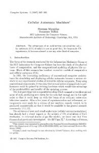
Age Addr Worksp Info Program Figure 3.1. Three neighbor colonies with their tracks

The codes ' between sets R; S used in our simulations will have a feature similar to the acceptance and rejection of Example 3.1. The set R will always have a special symbol called Vac, the vacant symbol. An element s 2 S will be called accepted by the decoding if ' (s) 6= Vac, otherwise it is called rejected. 3.3. Generalized cellular automata (abstract media). A block code ' could be used to de ne a code on con gurations between cellular automata M1 and M2 . Suppose that a con guration of M2 is given. Then we could de ne the con guration = ' ( )of M1 by setting for each cell x of and 0 i < Q, (Qx + i) = ' ( (x))(i): The decoding function would be de ned correspondingly. This de nition of decoding is, however, unsatisfactory for our purposes. Suppose that is obtained by encoding a con guration via ' as before, and is obtained by shifting : (x) = (x ? 1). Then the decoding of will return all vacant values since now the strings ( (Qx); ; (Qx + Q ? 1)) are not \real" colonies. However, it will be essential for error correction that whenever parts of a con guration form a colony, even a shifted one, the decoding should notice it. With our current de nition of cellular automata, the decoding function could not be changed to do this. Indeed, if is the con guration decoded from then (0) corresponds to the value decoded from ( (0); ; (Q ? 1)), and (1) to the value decoded from ( (Q); ; (2Q ? 1)). There is no site to correspond to the value decoded from ( (1); ; (Q)). Our solution is to generalize the notion of cellular automata. Let us give at once the most general de nition which then we will specialize later in varying degrees. The general notion is an abstract medium AMed(S; C; Configs; Evols; Trajs): Here, Configs is the set of functions : C ! S that are con gurations and Evols is the set of functions : C [0; 1?] ! S that are space-time con gurations of the abstract medium. Further, Trajs is the set of random space-time con gurations (; ) that are trajectories. In all cases that we will consider, the set Trajs will be given in a uniform way, as a function Traj(C) of C. The sets S, C, Configs and Evols are essentially super uous since the set Trajs de nes them implicitly|therefore we may omit them from the notation, so that eventually we may just write AMed(Trajs): Given media M1 ; M2 for the same S; C, we will write M1 M2


17

if Trajs1 Trajs2 . Let

M1 \ M2 be the medium whose trajectory set is Trajs1 \ Trajs2 . Let us now consider some special cases. 3.3.1. Cellular abstract media. All abstract media in this paper will be cellular: the sets Configs and Evols will be de ned in the way given here. The set S of local states will always include a distinguished state called the vacant state Vac. If in a con guration we have (x) 6= Vac then we will say that there is a cell at site x in . We will have a positive number B called the body size. In ordinary cellular automata, B = 1. For a site x, interval [x; x + B ?] will be called the body of a possible cell with base x. A function : C ! S is a con guration if the cells in it have non-intersecting bodies. Remark 3.3. Since not each site will be occupied by a cell, it is not even important to restrict the set of sites to integers; but we will do so for convenience. } A function : C [0; 1?] ! S is a space-time con guration if (a) (; t) is a space con guration for each t; (b) (x; t) is a right-continuous function of t; (c) Each nite time interval contains only nitely many switching times for each site x; A dwell period is a tuple (x; s; t1 ; t2 ) such that x is a site, s is a nonvacant state, and 0 t1 < t2 are times. The rectangle [x; x + B ?] [t1 ; t2 ?] is the space-time body of the dwell period. It is easy to see that the dwell periods in a space-time con guration have disjoint bodies. This completes the de nition of the sets Configs and Evols in cellular abstract media, the only kind of media used in this paper. Therefore from now on, we may write AMed(C; Trajs; B ): We may omit any of the arguments if it is not needed for the context. We will speak of a lattice con guration if all cells are at sites of the form iB for integers i. We can also talk about lattice space-time con gurations: these have space-time bodies of the form [iB; (i + 1)B ?] [jT; (j + 1)T ?] for integers i; j . A special kind of generalized cellular automaton is a straightforward rede nition of the original notion of cellular automaton, with two new but inessential parameters: a deterministic cellular automaton

CA(Tr ; B; T; C) is determined by B; T > 0 and a transition function Tr : S3 ! S. We may omit some obvious arguments from this notation. A lattice space-time con guration with parameters B; T is a trajectory of this automaton if (x; t) = Tr((x ? B; t ? T ); (x; t ? T ); (x + B; t ? T )) holds for all x; t with t T . For a space-time con guration let us write (3.2) Tr(; x; t; B ) = Tr((x ? B; t); (x; t); (x + B; t)): We will omit the argument B when it is obvious from the context. Probabilistic cellular automata and perturbations are generalized correspondingly as PCA(P; B; T; C); CA" (Tr ; B; T; C):

18

PETER GA CS

From now on, whenever we talk about a deterministic, probabilistic or perturbed cellular automaton we understand one also having parameters B; T . We will have two kinds of abstract medium that are more general than these cellular automata. We have a constant-period medium if in all its trajectories, all dwell period lengths are multiples of some constant T . Otherwise, we have a variable-period medium. 3.3.2. Block codes between cellular automata. In a cellular abstract medium with body size B , a colony of size Q is de ned as a set of cells x + iB for i 2 [0; Q ? 1]. Thus, the union of the cell bodies of body size B in a colony of size Q occupies some interval [x; x + QB ?]. A block code will be called overlap-free if for every string (s(0); : : : s(n ? 1)), and all i n ? Q, if both (s(0); : : : ; s(Q ? 1)) and (s(i + 1); : : : ; s(i + Q ? 1)) are accepted then i Q. In other words, a code is overlap-free if two accepted words cannot overlap in a nontrivial way. The code in Example 3.1 is overlap-free. All block-codes considered from now on will be overlap-free. Overlap-free codes are used, among others, in [18]. 3.3.3. Codes on con gurations. A block code ' of block size Q can be used to de ne a code on con gurations between generalized abstract media M1 and M2 . Suppose that a con guration of M2 , which is an AMed(QB ), is given. Then we de ne the con guration = ' ( ) of M1 , which is an AMed(B ), by setting for each cell x of and 0 i < Q, (x + iB ) = ' ( (x))(i): Suppose that a con guration of M1 is given. We de ne the con guration = ' ( ) of M2 as follows: for site x, we set (x) = ' (s) where (3.3) s = ( (x); (x + B ); : : : ; (x + (Q ? 1)B )): If is a con guration with = ' ( ) then, due to the overlap-free nature of the code, the value (x) is nonvacant only at positions x where (x) is nonvacant. If is not the code of any con guration then it may happen that in the decoded con guration ' ( ), the cells will not be exactly at a distance QB apart. The overlap-free nature of the code garantees that the distance of cells in ' ( ) is at least QB even in this case. 3.4. Block simulations. Suppose that M1 and M2 are deterministic cellular automata where Mi = CA(Tr i ; Bi ; Ti ), and ' is a block code with B1 = B; B2 = QB: The decoding function may be as simple as in Example 3.1: there is an Info track and once the colony is accepted the decoding function depends only on this part of the information in it. For each space-time con guration of M1 , we can de ne = ' () of M2 by setting (3.4) (; t) = ' ((; t)): We will say that the code ' is a simulation if for each con guration of M2 , for the trajectory (; ) of M1, such that (; 0; !) = ' ( ) for almost all !, the random space-time con guration (; ) is a trajectory of M2 . (We do not have to change here since the ! in (x; t; !) is still coming from the same space as the one in (x; t; !).) We can view ' as an encoding of the initial con guration of M2 into that of M1 . A space-time con guration of M1 will be viewed to have a \good" initial con guration (; 0) if the latter is ' ( ) for some con guration of M2 . Our requirements say that from every trajectory of M1 with good initial con gurations, the simulation-decoding results in a trajectory of M2 .


19

Let us show one particular way in which the code ' can be a simulation. For this, the function Tr 1 must behave in a certain way which we describe here. Assume that T1 = T; T2 = UT for some positive integer U called the work period size. Each cell of M1 will go through a period consisting of U steps in such a way that the Info eld will be changed only in the last step of this period. The initial con guration (; 0) = ' ( ) is chosen in such a way that each cell is at the beginning of its work period. By the nature of the code, in the initial con guration, cells of M1 are grouped into colonies. Once started from such an initial con guration, during each work period, each colony, in cooperation with its two neighbor colonies, computes the new con guration. With the block code in Example 3.1, this may happen as follows. Let us denote by r? ; r0 ; r+ the value in the rst 12 bits of the Info track in the left neighbor colony, in the colony itself and in the right neighbor colony respectively. First, r? and r+ are shipped into the middle colony. Then, the middle colony computes s = Tr 2 (r?1 ; r0 ; r1 ) where Tr 2 is the transition function or M2 and stores it on a memory track. (It may help understanding how this happens if we think of the possibilities of using some mail, memory and workspace tracks.) Then, in the last step, s will be copied onto the Info track. Such a simulation is called a block simulation. Example 3.4. Let us give a trivial example of a block simulation which will be applied, however, later in the paper. Given a one-dimensional transition function Tr(x; y; z ) with state space S, we can de ne for all positive integers Q an aggregated transition function Tr Q (u; v; w) as follows. The state space of of Tr Q is SQ. Let rj = (rj (0); : : : ; rj (Q ? 1)) for j = ?1; 0; 1 be three elements of SQ. Concatenate these three strings to get a string of length 3Q and apply the transition function Tr to each group of three consecutive symbols to obtain a string of length 3Q ? 2 (the end symbols do not have both neighbors). Repeat this Q times to get a string of Q symbols of S: this is the value of Tr Q (r?1 ; r0 ; r1 ). For M1 = CA(S; Tr; B; T ) and M2 = CA(SQ; Tr Q ; QB; QT ), the aggregation code Q de ned in Example 3.2 will be a block simulation of M2 by M1 with a work period consisting of U = Q steps. If along with the transition function Tr, there were some elds FS; G; : : : All also de ned then we de ne, say, the eld F in the aggregated cellular automaton as iQ=0?1 (F + ikSk). Thus, if r = r(0) t t r(Q ? 1) is a state of the aggregated cellular automaton then r:F = r(0):F t r(1):F t t r(Q ? 1):F. } 0 A transition function Tr is universal if for every other transition function Tr there are Q; U and a block code ' such that ' is a block simulation of CA(Tr 0 ; Q; U ) by CA(Tr ; 1; 1). Theorem 3.5 (Universal cellular automata). There is a universal transition function. Sketch of proof: This theorem is proved somewhat analogously to the theorem on the existence of universal Turing machines. If the universal transition function is Tr then for simulating another transition function Tr 0 , the encoding demarcates colonies of appropriate size with Addr = 0, and writes a string Table that is the code of the transition table of Tr 0 onto a special track called Prog in each of these colonies. The computation is just a table-look-up: the triple (r? ; r0 ; r+ ) mentioned in the above example must be looked up in the transition table. The transition function governing this activity does not depend on the particular content of the Prog track, and is therefore independent of Tr 0 . For references to the rst proofs of universality (in a technically dierent but similar sense), see [4, 26] Note that a universal cellular automaton cannot use codes similar to Example 3.1. Indeed, in that example, the capacity of the cells of M1 is at least the binary logarithm of the colony size, since

20

PETER GA CS

each colony cell contained its own address within the colony. But if M1 is universal then the various simulations in which it participates will have arbitrarily large colony sizes. The size Q of the simulating colony will generally be very large also since the latter contains the whole table of the simulated transition function. There are many special cellular automata M2 , however, whose transition function can be described by a small computer program and computed in relatively little space and time (linear in the size kS2k). The universal transition function will simulate these with correspondingly small Q and U . We will only deal with such automata. 3.5. Single-fault-tolerant block simulation. Here we outline a cellular automaton M1 that block-simulates a cellular automaton M2 correctly as long as at most a single error occurs in a colony work period of size U . The outline is very informal: it is only intended to give some framework to refer to later: in particular, we add a few more elds to the elds of local states introduced earlier. For simplicity, these elds are not de ned here in a way to make the cellular automaton separable in the sense de ned in 2.2.1. They could be made so with a few adjustments but we want to keep the introduction simple. The automaton M1 is not universal, i.e. the automaton M2 cannot be chosen arbitrarily. Among others, this is due to the fact that the address eld of a cell of M1 will hold its address within its colony. But we will see later that universality is not needed in this context. The cells of M1 will have, besides the Addr eld, also a eld Age. If no errors occur then in the i-th step of the colony work period, each cell will have the number i in the eld Age. There are also elds called Mail, Info, Work, Hold, Prog. The Info eld holds the state of the represented cell of M2 in three copies. The Hold eld will hold parts of the nal result before it will be, in the last step of the work period, copied into Info. The role of the other elds is clear. The program will be described from the point of view of a certain colony C . Here is an informal description of the activities taking place in the rst third of the work period. 1. From the three thirds of the Info eld, by majority vote, a single string is computed. Let us call it the input string. This computation, as all others, takes place in the workspace eld Work; the Info eld is not aected. The result is also stored in the workspace. 2. The input strings computed in the two neighbor colonies are shipped into C and stored in the workspace separately from each other and the original input string. 3. The workspace eld behaves as a universal automaton, and from the three input strings and the Prog eld, computes the string that would be obtained by the transition function of M2 from them. This string will be copied to the rst third of the Hold track. In the second part of the work period, the same activities will be performed, except that the result will be stored in the second part of the Hold track. Similarly with the third part of the work period. In a nal step, the Hold eld is copied into the Info eld. The computation is coordinated with the help of the Addr and Age elds. It is therefore important that these are correct. Fortunately, if a single fault changes such a eld of a cell then the cell can easily restore it using the Addr and Age elds of its neighbors. It is not hard to see that with such a program (transition function), if the colony started with \perfect" information then a single fault will not corrupt more than a third of the colony at the end of the work period. On the other hand, if two thirds of the colony was correct at the beginning of the colony work period and there is no fault during the colony work period then the result will be \perfect". 3.6. General simulations. The main justi cation of the general notion of abstract media is that it allows a very general de nition of simulations: a simulation of abstract medium M2 by abstract


medium M1 is given by a pair

21

(' ; ) where is a mapping of the set of space-time con gurations of M1 into those of M2 (the decoding), and ' is a mapping of the set of con gurations of M2 to the set of con gurations of M1 (the encoding for initialization). Let us denote = (): We require, for each trajectory for which the initial con guration has the encoded form (; 0) = ' ( ), that is a trajectory of M2 with (; 0) = . A simulation will be called local, if there is a nite space-time rectangle V = I [?u; 0] such that ()(w; t) depends only on ((w; t) + V ). Together with the shift-invariance property, the locality property implies that a simulation is determined by a function de ned on the set of con gurations over V . All simulations will be local unless stated otherwise. Corollary 7.3 gives an example of non-local simulation. If u = 0 then the con guration (; t) depends only on the con guration (; t). In this case, the simulation could be called \memoryless". For a memoryless simulation, the simulation property is identical to the one we gave at the beginning of Subsection 3.4. Our eventual simulations will not be memoryless but will be at least non-anticipating: we will have u > 0, i.e. the decoding looks back on the space-time con guration during [t ? u; t], but still does not look ahead. In particular, the value of (; 0) depends only on (; 0) and therefore the simulation always de nes also a decoding function ' on space-con gurations. From now on, this decoding function will be considered part of the de nition of the simulation, i.e. we will write = (' ; ' ; ): Suppose that a sequence M1 ; M2 ; : : : of abstract media is given along with simulations 1 ; 2 ; : : : such that k is a simulation of Mk+1 by Mk . Such a system will be called an ampli er. Ampli ers are like renormalization groups in statistical physics. Of course, we have not seen any nontrivial example of simulation other than between deterministic cellular automata, so the idea of an ampli er seems far-fetched at this moment. 3.6.1. Simulation between perturbations. Our goal is to nd nontrivial simulations between cellular automata M1 and M2 , especially when these are not deterministic. If M1 ; M2 are probabilistic cellular automata then the simulation property would mean that whenever we have a trajectory (; ) of M1 the random space-time con guration decoded from would be a trajectory of M2 . There are hardly any nontrivial examples of this sort since in order to be a trajectory of M2 , the conditional probabilities of ' () must satisfy certain equations de ned by P2 , while the conditional probabilitiees of satisfy equations de ned by P1 . There is more chance of success in the case when M1 and M2 are perturbations of some deterministic cellular automata since in this case, only some inequalities must be satis ed. The goal of improving reliability could be this. For some universal transition function Tr 2 , and at least two different initial con gurations i (i = 0; 1), nd Tr 1 ; Q; U; c with B1 = B , B2 = BQ, T1 = T , T2 = TU and a block simulation 1 such that for all " > 0, if "1 = ", "2 = c"2 and Mk is the perturbation CA"k (Tr k ; Bk ; Tk ; Z) then 1 is a simulation of M2 by M1 . The meaning of this is that even if we have to cope with the fault probability " the simulation will compute Tr 2 with a much smaller fault probability c"2 . The hope is not unreasonable since in Subsection 3.5, we outlined a single-fault-tolerant block simulation while the probability of several faults happening during one work period is only of the order of

22

PETER GA CS

(QU")2 . However, it turns out that the only simply stated property of a perturbation that survives noisy simulation is a certain initial stability property (see below). 3.6.2. Error-correction. Even if the above goal can be achieved, the reason for the existence of the simulated more reliable abstract medium is to have feedback from it to the simulating one. The nature of this feedback will be de ned in the notion of error-correction to whose de nition now we proceed. Let us call the set (3.5) 0 = f0; 1; #; g the standard alphabet. Symbol # will be used to delimit binary strings, and will serve as a \don'tcare" symbol. Each eld F of a cell state such that the eld size is even, can be considered not only a binary string but a string of (half as many) symbols in the standard alphabet. If r; s are strings in (0 )n then rs will mean that s(i) = r(i) for all 0 i < n such that r(i) 6= . Thus, a don't-care symbol r(i) imposes no restriction on s in this relation. There will be two uses of the don't-care symbol. The more important use will come in de ning the code used for error-correction in a way that it requires the correction of only those parts of the information in which correction is desirable. The less important use is in de ning the notion of \monotonic output": namely, output that contains more and more information as time proceeds. This is convenient e.g. for continuoustime cellular automata, where it is dicult to say in advance when the computation should end. For codes ' ; , we will write ' if for all s we have (s) ' (s). Let us de ne the notion of error-correction. Let = (' ; ' ; ) be a simulation whose encoding ' is a block code with block size Q, between abstract cellular media Mi (i = 1; 2). Let Ti > 0 (i = 1; 2) be some parameters, and ' ' a block code of blocksize Q. We say that has the "-error-correction property with respect to ' ; T1; T2 if the following holds for every con guration of M2 and every trajectory (; ) of M1 with (; 0) = ' ( ). Let = () and let x1 ; x2 be sites where x1 has address a in the Q-colony with base x2 , let t0 be some time. Let E be the event that (x2 ; ) is nonvacant during [t0 ? T2 =3; t0] and let E 0 be the event that for each t in [t0 ? T1 =3; t0] there is a t0 in [t0 ? T2 =3; t] with ' ( (x2 ; t0 ))(a) (x1 ; t): Then Probf E \ :E 0 g < ". Informally, this means that for all x1 ; x2 ; a in the given relation, the state (x1 ; t) is with large probability what we expect by encoding some (x2 ; t0 ) via ' and taking the a-th symbol of the codeword. Error-correction is only required for a code ' ' since ' determines the value of many elds as a matter of initialization only: these elds need not keep their values constant during the computation, and therefore ' will assign don't-care symbols to them. The code ' will thus generally be obtained by a simple modi cation of ' . Example 3.6. Let B1 = 1; B2 = Q; T1 = 1; T2 = U


t0

xs2

x1 = x2 + aB

' }|

z

6

t ? T1 =3

q

23

q

q

q

q

q

q

q

q

q

>

s

t t0 ? T1=3 {

q

q

q

q

q

t0 x2 + QB q

time

t0 ? T2 =3 Figure 3.2. Error correction

for some U > Q. Assume that for k = 1; 2, our media Mk are cellular generalized media with body sizes Bk and state spaces Sk. Assume further that M2 has at least a eld F 2 with jF 2 j Q=3 and M1 has at least the elds F 1 ; Addr ; Age, with jF 1 j = 2. For a state s 2 S2, let the string

s0 = ' (s) 2 SQ1 be de ned as follows. Take the binary string s:F 2 , repeat it 3 times, pad it with 's to a string of size Q of the standard alphabet: let this be a string (f (0); : : : ; f (Q ? 1)). Now for each address b, let s0 (b):F 1 = f (b); s0 (b):Addr = b; s0 (b):Age = 0; and let all other elds of s0 (b) be lled with 's. The de nition of s00 = ' (s) starts as the de nition of s0 with the only dierence that set s00 (b):Age = . Thus, the code ' (s) encodes a redundant version of s:F 2 onto the F 1 track of the block s0 and initializes the Addr and Age tracks to the values they would have at the beginning of a work period. The code ' (s) leaves all tracks other than F 1 and Addr undetermined, since it will have to be compared with the state of the colony also at times dierent from the beginning of the work period. }

PETER GA CS

24

Suppose that an ampli er (Mk ; k )k1 is given along with the sequences 'k ; Tk ; "00k . We will call this structure an error-correcting ampli er if for each k, the simulation k has the "00k - error correction property with respect to 'k , Tk , Tk+1 . 3.7. Remembering a bit: proof from an ampli er assumption. The following lemma will be proved later in the paper. Lemma 3.7 (Initially Stable Ampli er). We can construct the following objects, for k = 1; 2; : : : . (a) Media Mk over state space Sk, simulations P k = ('k ; 'k ; k ) and sequences 'k , "00k , Tk 00 forming an "k - error correcting ampli er P with k "00k < 1=6. (b) (Initial stability) Parameters "k ; B1 with k "k < 1=6, transition function Tr 1 and two con gurations 0 ; 1 such that, de ning u1 = u , uk+1 = 'k (uk ) for u = 0; 1, we have M1 = CA"1 (Tr 1 ; B1 ; T1 ; Z): Further, for each k; u, for each trajectory of Mk with (; 0) = uk , for all t < Tk , for each site x, we have Probf (x; t) 6= (x; 0) g < "k : (c) Parameters Qk such that the codes 'k are block codes with block size Qk . (d) (Broadcast) Fields F k for the state spaces Sk such that for each k, for each address a 2 [0; Qk ? 1] and state s 2 Sk+1, for each u 2 f0; 1g and site x we have (3.6) uk (x):F k = u; (3.7) s:F k+1 'k (s)(a):F k : Equation (3.6) says for the con gurations uk , (obtained by decoding from the initial con guration u ) in each cell of medium Mk , eld F k has value u. Equation (3.7) says the following. Assume for symbol s 2 Sk+1 we have s:F k+1 = u 6= . Then the encoding function ' encodes s into a colony of Qk symbols r0 ; : : : ; rQk ?1 such that for each a, we have sa :F k = u. Thus, the F k+1 eld of s gets \broadcast" into the F k eld of each symbol of the code of s. This way, even if property (3.6) were assumed only for a xed level k, property would (3.7) imply it for all i < k. Let us use this lemma to prove the rst theorem. Proof of Theorem 2.5. Let us use the ampli er de ned in the above lemma. Let 1 be a trajectory of the medium M1 with initial con guration u . Let k be de ned by the recursion k+1 = k (k ). Let (x1 ; t1 ) be a space-time point in which we want to check (x1 ; t1 ):F 1 = u. There is a sequence of points x1 ; x2 ; : : : such that xk+1 is a cell of k+1 (; 0) containing xk in its body with some address bk . There is a rst n with t1 < Tn=3. Let Fk P be the eventPthat k (xk ; t):F k = u for t in [t1 ? Tk =3; t1]. The theorem follows from the bounds on k "k and k "00k and from Probf :(F1 \ \ Fn) g "n +

(3.8) To prove this inequality, use

:(F1 \ \ Fn) = :Fn [

n[ ?1 k=1

nX ?1 k=1

"00k :

(:Fk \ Fk+1 ):

By the construction, n (xn ; 0):F n = u. Since the duration of [0; t1] is less than Tn we have Probf n(xn ; t1 ) 6= n (xn ; 0) g < "n by the initial stability property, proving Probf :Fn g "n . The error-correction property and the broadcast property imply Probf Fk+1 \ :Fk g "00k .


25

Age Addr Worksp Prog

Info

Worksp Addr

Age

Info Prog

Figure 4.1. Fields of a cell simulated by a colony

4. Hierarchy 4.1. Hierarchical codes. The present section may seem a long distraction from the main course of exposition but many readers of this paper may have diculty imagining an in nite hierarchical structure built into a con guration of a cellular automaton. Even if we see the possibility of such structures it is important to understand the great amount of exibility that exists while building it. Formally, a hiearchy will be de ned as a \composite code". Though no decoding will be mentioned in this subsection, it is still assumed that to all codes ' mentioned, there belongs a decoding function ' with ' (' (x)) = x. 4.1.1. Composite codes. Let us discuss the hierarchical structure arising in an ampli er. If '; are two codes then ' is de ned by (' ) ( ) = ' ( ( )) and (' ) ( ) = (' ( )). It is assumed that and are here con gurations of the appropriate cellular automata, i.e. the cell body sizes are in the corresponding relation. The code ' is called the composition of ' and . For example, let M1 ; M2; M3 have cell body sizes 1; 31; 312 respectively. Let us use the code ' from Example 3.1. The code '2 = ' ' maps each cell c of M3 with body size 312 into a \supercolony" of 31 31 cells of body size 1 in M1. Suppose that = '2 ( ) is a con guration obtained by encoding from a lattice con guration of body size 312 in M3 , where the bases of the cells are at positions ?480 + 312i. (We chose -480 only since 480 = (312 ? 1)=2 but we could have chosen any other number.) Then can be broken up into colonies of size 31 starting at any of those bases. Cell 55 of M1 belongs to the colony with base 47 = ?480 + 17 31 and has address 8 in it. Therefore the address eld of (55) contains a binary representation of 8. The last bit of this cell encodes the 8-th bit the of cell (with base) 47 of M2 represented by this colony. If we read together all 12 bits represented by the Info elds of the rst 12 cells in this colony we get a state (47) (we count from 0). The cells with base ?15 + 31j for j 2 Z with states (?15 + 31j ) obtained this way are also broken up into colonies. In them, the rst 5 bits of each state form the address and the last bits of the rst 12 cells, when put together, give back the state of the cell represented by this colony. Notice that these 12 bits were really drawn from 312 cells of M1 . Even the address bits in (47) come from dierent cells of the colony with base 47. Therefore the cell with state (55) does not contain information allowing us to conclude that it is cell 55. It only \knows" that it is the 8-th cell within its own colony (with base 47) but does not know that its colony has address 17 within its supercolony (with base ?15 31) since it has at most one bit of that address. 4.1.2. In nite composition. A code can form composition an arbitrary number of times with itself or other codes. In this way, a hierarchical, i.e. highly nonhomogenous, structure can be de ned using cells that have only a small number of states. A hierarchical code is given by a sequence (4.1) (Sk; Qk ; 'k )k1

26

PETER GA CS

where Sk is an alphabet, Qk is a positive integer and 'k : Sk+1 ! SQk k is an encoding function. Since Sk and Qk are implicitly de ned by 'k we can refer to the code as just ('k ). We will need a composition '1 '2 of the codes in a hierarchical code since the the de nition of the initial con guration for M1 in the ampli er depends on all codes 'i . What is the meaning of this? We will want to compose the codes \backwards", i.e. in such a way that from a con guration 1 of M1 with cell body size 1, we can decode the con guration 2 = '1 ( 1 ) of M2 with cell body size B2 = Q1 , con guration 3 = '2 ( 2 ), of M3 with body size B3 = Q1 Q2 , etc. Such constructions are not unknown, they were used e.g. to de ne \Morse sequences" with applications in group theory as well in the theory of quasicrystals ([18, 24]). Let us call a sequence a1 ; a2 ; : : : with 0 ak < Qk non-degenerate for Q1 ; Q2 ; : : : if there are in nitely many k with ak > 0 and in nitely many k with ak < Qk ? 1. The pair of sequences (4.2) (Qk ; ak )1 k=1 with non-degenerate ak will be called a block frame of our hierarchical codes. All our hierarchical codes will depend on some xed block frame, ((Qk ; ak )), but this dependence will generally not be shown in the notation. Remarks 4.1. 1. The construction below does not need the generality of an arbitrary non-degenerate sequence: we could have ak = 1 throughout. We feel, however, that keeping ak general makes the construction actually more transparent. 2. It is easy to extend the construction to degenerate sequences. If e.g. ak = 0 for all but a nite number of k then the process creates a con guration in nite in right direction, and a similar construction must be added to attach to it a con guration in nite in the left direction.

}

For a block frame ((Qk ; ak )), a nite or in nite sequence (s1 ; a1 ); (s2 ; a2 ); : : : will be called tted to the hierarchical code ('k ) if 'k (sk+1 )(ak ) = sk holds for all k. For a nite or in nite space size N , let B1 = 1; (4.3) Bk = Q1 Qk?1 for k > 1; (4.4) K = K (N ) = sup k + 1; Bk i 1. We have +1 (ok+1 ))(ak ) = k (ok ) (4.10) kk+1 (ok ) = 'k (kk+1 k where the rst equation comes by de nition, the second one by ttedness. The encoding conserves this relation, so the partial con guration ki +1 (ok+1 +[0; Bk+1 ? 1]) is an extension of ki (ok +[0; Bk ? 1]). Therefore the limit i = limk ki exists for each i. Since (ak ) is non-degenerate the limit extends over the whole set of integer sites. Though 1 above is obtained by an in nite process of encoding, no in nite process of decoding is needed to yield a single con guration from it: at the k-th stage of the decoding, we get a con guration k with body size Bk . 4.1.3. Controlling, identi cation. The need for some freedom in constructing in nite tted sequences leads to the following de nitions. For alphabet S and eld F let S:F = f w:F : w 2 S g: Then, of course, kS:Fk = jF j. Let D = fd0 ; : : : ; djDj?1 g [0; Q ? 1] be a set of addresses with di < di+1 . For a string s, let s(D):F be the string of values (s(d0 ):F ; : : : ; s(djDj?1 ):F) so that s:F = s([0; Q ? 1]):F : Field F controls an address a in code ' via function : S1:F ! S1 if (a) For all r 2 S1:F there is an s with ' (s)(a):F = r; in other words, ' (s)(a):F runs through all possible values for this eld as s varies. (b) For all s we have ' (s)(a) = (' (s)(a):F); in other words, the eld ' (s)(a):F determines all the other elds of ' (s)(a). From now on, in the present subsection, whenever we denote a eld by F k and a code by 'k we will implicitly assume that F k controls address ak in 'k unless we say otherwise. (The index k in F k is not an exponent.) Suppose that elds F 1 ; F 2 are de ned for cellular automata M1 and M2 between which the code ' with blocksize Q is given. Suppose that set D satis es jDj = jF 2 j=jF 1 j. We say that in ' , eld F 1 over D is identi ed with F 2 if in any codeword w = ' (s), the string w(d0 ):F 1 t t w(djDj?1 ):F 1 is identical to s:F 2 . Conversely, thus w(di ):F 1 = s:F 2 ([ijF 1 j; (i + 1)jF 1 j ? 1]). The identi cation of F 2

PETER GA CS

28

Age 1 Addr 1 1 Worksp Prog 2

Info 2 0

Worksp2 Addr 2

Age 2

Info 1 Prog 1

Figure 4.2. Assume that in the code of this gure, Addr, Age and Worksp are

constant and Prog 1 has always 0 in its position 4. Then address 4 is controlled by Info 1 , and Info 2 is identi ed with Info 1 over the addresses 4-17.

with F 1 over D implies that if a simulation has error-correction in F 1 over D then the information restored there is s:F 2 . Example 4.3. Consider the simulation outlined in Subsection 3.5, and let us call the encoding ' . Let F 1 be the Info eld of M1 : we denote it by Info 1 . Assume further that the simulated medium M2 is of a similar type, so it has an Info 2 eld. Assume for simplicity 6 j Q; jInfo 1 j = 2; jInfo 2 j = Q=3: The Info 1 eld of cells in interval [0; Q=3 ? 1] of a simulating colony represents the whole state of a simulated cell of M2 . The Info 1 eld on [Q=3; Q ? 1] is only used for redundancy. Only a segment of the Info 1 eld of [0; Q=3 ? 1], say the one on [0; Q=6 ? 1] is used to represent Info 2 of the simulated cell. The rest is used for encoding the other elds. Hence Info 1 on [0; Q=6 ? 1] is identi ed with Info 2 in our code ' . Let s0 = ' (s)(1) be the state of the cell with address 1 of a colony of M1 which is the result of encoding state s of M2 . Let s0 :Info 1 be the third and fourth bits of s:Info 2 , s0 :Addr = 1, and s0 :F = 0 for all elds dierent from these two. Then Info 1 controls address 1 in the code ' . } If for each address a, the eld F 1 over fag is identi ed with F 2 then we say that F 2 is broadcast to F 1 (since this means that the code copies the value of s:F 2 into the F 1 eld of each cell of ' (s)). Let us be given (4.11) = ((Sk; Qk ; 'k ; F k ; k ; ak ) : k 1) where 1 ak Qk ? 2, such that in code 'k , (a) F k over fak g is identi ed with F k+1 ; (b) F k controls address ak for 'k via k ; Such a system of elds F k will be called a primitive shared eld for the hierarchical code ('k ). If also each code 'k , broadcasts F k+1 into F k then we will say that the elds F k form a broadcast eld. Note that the eld still controls only a single address ak . The Main bit eld mentioned in Subsection 3.1 would be an example. Proposition 4.4. For any hierarchical code with primitive shared eld given as in (4.11) above, for all possible values u1 2 S1:F 1 the in nite sequence (sk ; ak )k1 with sk = k (u1 ) is tted. The proof is immediate from the de nitions.


29

Let us denote the con gurations 1 ; k1 that belong to this tted in nite sequence according to Proposition 4.2 (and its proof) by 1 = ?(u1 ; ) = ?(u1 ); (4.12) k1 = ?(u1 ; k; ) = ?(u1; k): 4.1.4. Coding an in nite sequence. Let us show now how a doubly in nite sequence of symbols can be encoded into an in nite starting con guration. Let us be given (4.13) = (Sk; Qk ; 'k ; F k ; qk ; k ; ak )k1 where 2 qk Qk and the sequence ak is non-degenerate, such that in code 'k , (a) F k over [0; qk ? 1] is identi ed with F k+1 ; (b) F k controls address ak for 'k via k ; Such a system will be called a shared eld for the elds F k , and the hierarchical code ('k ), and the elds F k will be denoted as F k ( ): The identi cation property implies that for all 0 a < qk , we have (4.14) 'k (s)(a):F k = s:F k+1 ([ajF k j; (a + 1)jF k j ? 1]): Example 4.5. Let us show some examples of codes 'k in which F k over [0; qk ? 1] is identi ed with F k+1 . A code = ( ; ) with : RQ ! S will be called d-error-correcting with blocksize Q if for all u; v, if u diers from (v) in at most d symbols then (u) = v. Assume that both R and S are of the form f0; 1gn (for dierent n). A popular kind of error-correcting code are codes such that is a linear mapping when the binary strings in S and RQ are considered vectors over the eld f0; 1g. These codes are called linear codes. It is sucient to consider linear codes which have the property that for all s, the rst jS j bits of the codeword (s) are identical to s: they are called the information bits. (If a linear code is not such, it can always be rearranged to have this property.) In this case, the remaining bits of the codeword are called error-check bits, and they are linear functions of s. Applying such linear codes to our case, for s 2 Sk+1, let w = 'k (s): Then we will have t0a 0, for any trajectory of Tr over Z with (; 0) of the form Init(%) (see (5.4)), satisfying 2jSupp(; t)j s, for any nite K h0 (t) and possibly in nite N satisfying Supp(; t) Visible(K; N ), for any trajectory of CA" (Tr 0 ) over C = ZN with initial con guration ?(%; K; ), for all y 2 Supp(; t), we have Probf (y; t):Output 6 (X (y; K; ); h1(t)):Output1 g < d1 ": The code can be chosen to have X (y; K; ) = y and jVisible(K; N )j = N . Thus, to nd a computation result (y; u) of CA(Tr), from some input, we must do the following. Find a bound s on 2jSupp(; t)j (the amount of space required by the computation if we put the origin somewhere into the input), then the level K h0 (t) on which the trajectory of the faulttolerant automaton CA" (Tr 0 ) carries out the computation to the desired stage u with the desired reliability until step t. Embed the input into a con guration % whose support contains 0. Encode % into an initial con guration ?( (; 0); K ) in a space whose size N is large enough to have Supp(; t) Visible(K; N ). \Run" the trajectory until time h1 (t), (it will be programmed to keep the active level at K ), and nally look up the result in site X (y; K ). Due to monotonic output, it is always possible to look up the result later. If you look at it too early the worst thing that can happen is that it will still be unde ned. The function h1 (t)=t measures time redundancy while X (y; h0(t))=y measures space redundancy (which, as the theorem says, can be made constant). The above theorem strengthens the result of [10] by eliminating the need for the decoding of the computation result: we just have to look in the right place for it. In two dimensions such a construction was given in [11]. The time redundancy in that paper is O(log2+ (NL)) where N; L are the upper bounds on the space and time requirements of the computation. We believe that this two-dimensional time redundancy can be reduced to log1+ (NL).

44

PETER GA CS

5.2.1. Adaptive encoding. Theorem 5.8 is not entirely satisfactory since its initial encoding (the active level) depends on the knowledge of a time and space bound on the whole computation. It is possible to remove this limitation. Instead of formulating the theorem, we just describe the idea of the construction. The initial encoding populates the space with cells of Mk for all k < K (N ) where N is the space size. Chose a level k1 of encoding for the computation input depending only on the size of the input. For an appropriately chosen (universal) increasing sequence (Lk ), after Lk computation steps have been simulated, the active level will be raised from k to k + 1. The parameters k1 and (Lk ) are chosen to guarantee with high probability that none of level k cells involved in the actual computation will fail before the level will be raised to k + 1. 5.2.2. Self-organization. In the just-discussed hierarchical fault-tolerant computations, the initial con guration is highly non-uniform since it encodes the hierarchy of simulations described above. If we forgo this initialization then the hierarchy must apparently be built up spontaneously. Initially, all sites in the media M2 ; M3 ; : : : could be vacant but cells could emerge spontaneously, as lower-level cells organize themselves (with the help of some randomness) into colonies simulating higher-level cells. We call this feature self-organization , but postpone its formal de nition a few sections later.


45

6. Media An abstract medium has been de ned in 3.3 as essentially a set of stochastic processes called its trajectories. Let us narrow this category somewhat. The kind of abstract medium considered in this paper will simply be called a medium. We will also restrict the kind of simulations among media to such mappings that by their very form will obviously be simulations: they will be called canonical simulations. 6.1. Trajectories. Here, we will show in what form the set of trajectories of a medium will be given. 6.1.1. Weak trajectories. In de ning the conditions making up a medium we will make use of inequalities of the form Eg b where g is an event function (as de ned in Subsection 2.3), measurable in A(V ) for some rectangle V. Example 6.1. Let V = [a1 +; a2] [t+; u], B < d = 0:2(a2 ? a1 ). Suppose that we are given some r 2 S3, s 2 S. Let g = 1 if there is a space-time point (x; t0 ) in V , and an " < d such that (x + iB; t) = ri for i = ?1; 0; 1 during [t0 ? "; t0?] and (x; t0 ) = s. Thus, the event g = 1 marks a certain kind of transition in the window. } A medium will be given by many such conditions. Let us x an arbitrary countable set T which will be called the set of condition types. A medium is given as (6.1) M = Med(S; C; g(; ; ); b()): Here, S is the set of possible local states and C is the set of possible cell sites. The space C can also be omitted whenever it is clear from the context. For all types 2 T and rational rectangles V , the medium assigns an event function g(; V; ) and a bound b() 2 [0; 1]. (We do not insist that g(; V; ) be measurable in A(V ) though usually this will be the case.) Therefore from now on, a local condition will be de ned as a pair (; V ): The set S is determined by g implicitly. Also, generally local conditions will only be de ned for small V , and in a translation-invariant way (in space, but only almost so in time since the time 0 is distinguished). Therefore one and the same pair g; b can serve for all suciently large nite spaces C as well as the in nite space, just like with deterministic cellular automata, where the same transition function determines trajectories in nite spaces as well as the in nite space. When we are given media M1 ; M2; : : : then gi (); bi () automatically refer to Mi . Two local conditions are disjoint when their rectangles are. A random space-time con guration will be called a weak trajectory if for each time u 0, for each set of disjoint local conditions (i ; Vi )iN with mini t Vi u, if h is an event function over Au then Y Y (6.2) E(h g(i; Vi ; )) Eh b(i ): i

i

This says that we can multiply the probabilities of violating local conditions in disjoint windows, i.e. that these violations happen \independently".

PETER GA CS

46

6.1.2. Trajectories. The media we are going to be interested in have these three types of condition. (1) One type recognizes in V a certain kind of value called \damage", and has b = " for some small "; (2) One type recognizes if there is no damage in V and the transition does not occur according to a certain transition function. This has b = 0. (3) One type corresponds to some \coin tossing" event, and has b = 0:5 + "0 for a suitable "0 . If we need coin-tossing (we need it only for the results on self-organization) then we must also consider certain sets of conditions that are chosen randomly. A random local condition is a (measurable) function (; V ()) assigning a local condition to each space-time con guration . We recall the de nition of stopping times from the theory of stochastic processes, specialized to our present needs. A real random variable with values in [0; 1?] is a stopping time derived from if for each t the event t is in At . Let A be the algebra of events A with the property that A \ f tg 2 At . Assume that for each t in [0; 1?] there is random variable V t () measurable in At with values that are rational rectangles with t V t () [t; 1] and such that with probability 1 the function V t () is right semi-continuous in t. This will be called a rectangle process derived from . We mention the following well-known fact from the theory or stochastic processes: Theorem 6.2 (see [21]). V is a random variable measurable in A . We will omit the words \derived from " when they are clear from the context. A random-stopping local condition is given by a triple (6.3) (; V t (); ) where is a type, V t () is a rectangle process and is a stopping time, both derived from . This condition is supposed to express the bound Eg(; V ; ) b(): For some nite set N of indices, let us now be given a sequence (6.4) (i ; Vit ; i )i2N of random-stopping local conditions. It is is called a system of disjoint random local conditions if (for almost all ) all the rectangles Vii () are disjoint, and there is a constant upper bound on the i and a constant segment containing all s Vit . A random space-time con guration will be called a trajectory if for each set of disjoint random local conditions as in (6.4) with i u, if h is an event function over Au then (6.5)

Y

Y

i

i

E(h g(i; )) Eh b(i )

where ? (6.6) g(i; ) = g i ; V i () (); : This also says that we can multiply the probabilities of violating local conditions in disjoint windows, but requires that this be even true if the windows are chosen by random stopping rules.


time

47

6

V11 1

V22

V33

2 3

Figure 6.1. A system of disjoint random local conditions

6.1.3. Examples of simple media. Example 6.3. The rst example will show how a PCA ts into this framework. Let us be given a probabilistic cellular automaton PCA(P; B; T ). For each state vector r 2 S3 and state s, let us form type (s; r).This condition type says that the transition rules are obeyed at times of the form nT . Then for cell x, time t of the form nT with n > 0, let ? g (s; r); fxg [t ? T +; t]; = f(x + iB; t ? T ) = ri (i = ?1; 0; 1); (x; t) = sg; (6.7) b((s; r)) = P(s; r): For all cells x and rational times u we de ne some new type = (x; u)by b( (x; u)) = 0 and ? g (x; u); f(x; u)g; = f (x; u) 6= (x; T bu=T c) g: This condition says that (x; u) = (x; T bu=T c) with probability 1. For all other combinations ; V we set g(; V; ) = 0. It is easy to see that the trajectories of PCA(P; B; T ) are trajectories of the medium de ned this way. } Example 6.4. The new conditions introduced below are \loosened-up" versions of the above ones since it is not always desirable to be as restrictive. Let us be given a probabilistic cellular automaton PCA(P; B; T ). For each set of states E , and state vector r = (r?1 ; r0 ; r1 ) let

P(E; r) =

X

q2E

P(q; r):

Let K be the set of functions K : S3 ! 2S such that (6.8) K (r) f s 6= r0 : P(s; r) > 0 g: For a space-time trajectory and a K 2 K let us write K (x; t; ) = K ((x ? B; t); (x; t); (x + iB; t)):

48

PETER GA CS

For all K 0 ; K 00 2 K with K 0 K 00 (i.e. K 0 (r) K 00 (r) for all r), let 00 (r); r) _ c(K 0 ; K 00 ) = PP((K K 0 (r); r) r be the least upper bound, over r, on the conditional probability of getting into the set K 00 (r) provided we get into the set K 00 (r). For each pair of such functions K 0 K 00 let us form the type = (K 0 ; K 00 ): For each cell x and u v of the form nT , let us form the rectangle V = fxg [u+; v]. For each such pair ; V let g(; V; ) = 1 if there is a rst t 2 [u+; v] with (x; t) 2 K 0(x; t ? T; ) and in it, we have (x; t) 2 K 00 (x; t ? T; ). Also, let b() = c(K 0; K 00 ). } Proposition 6.5. If M is the medium de ned by the conditions above then PCA(P; B; T ) M . Proof sketch. The statement follows by a standard argument from the strong Markov property of the Markov process PCA(B; B; T ) (see [21]). Example 6.6. Consider a continuous-time cellular automaton CCA(R; B ). For any functions K; K 0; K 00 2 K as in Example 6.4, let X R(K; r) = R(q; r); q2K

c(K 0; K 00 ) =

_ r

R(K 00(r); r) : R(K 0(r); r)

We de ne each (K 0 ; K 00 ), V = fxg [u+; v] and g(; V; ) as before, but now for all rational

u < v.

}

Theorem 6.7. Every trajectory of CCA(R; B) is a trajectory of the medium de ned in the above example. Proof sketch. As P in 2.4.1, for a small > 0, let M = PCA(P; B; ) with P(s; r) = R(s; r) when s 6= r0 and 1 ? s0 6=r0 R(s0 ; r) otherwise. Then a transition to the limit ! 0 in Proposition 6.5 completes the proof. The transition uses the fact that trajectories of M () converge in distribution to trajectories of CCA(R; B ). Remark 6.8. Of course in both Proposition 6.5 and in Theorem 6.7, instead of the rst time with switching into K 0 we could have asked about the second time, or the third time, etc. } 6.2. Canonical simulations. 6.2.1. De nition of canonical simulations. Let us introduce a special kind of simulation, that establishes certain relations between the local conditions of the media and thus makes it easier to prove it is a simulation. Let M1 ; M2 be media and let ' be a mapping from the space-time con gurations of M1 into the evolutions of M2: we will write = ' (). We say that ' is the map for a canonical simulation if the following holds. Let (; V ) be any local condition for M2 . Then there is a system of random local conditions ? (6.9) (; i; j ); W t (; i; j; V; ); (; i; j; V; ) with i = 1; : : : ; n(), j = 1; : : : ; k(; i), (6.10) inf t V (; i; j; V; );


49

such that for each xed i, the subsystem containing elements for that i forms a system of disjoint random local conditions with W t (; i; j; V; ) V , and, de ning W (; i; j; V; ) = W (;i;j;V;)(; i; j; V; ); (6.11) g1 (; i; j; V; ) = g1 ( (; i; j ); W (; i; j; V; ); ); we have XY g1 (; i; j; V; ); g2 (; V; ) i j (6.12) XY b1 ( (; i; j )): b2 () i

j

A simulation map will be called a deterministic canonical simulation when the system in (6.9) is deterministic: neither (; i; j; V; ) nor W t (; i; j; V; ) depends on . Under the condition mentioned in the de nition of weak trajectories (see (6.2)), we will be able to provide deterministic canonical simulations and this is why weak trajectories are sucient. Canonical simulations are \cooked up" to make the following theorem true. Theorem 6.9 (Canonical Simulation). If ' is a canonical simulation map then for each trajectory of M1, the expression ' () de nes a trajectory of M2. Proof. Let be a trajectory of M1 and (l ; Vlt ; l )l2N a system of disjoint random local conditions in M2 . Let u be some time such that l u for each l, and let h be an event function measurable in Au . We must show Y Y E? h g2(l; ) Eh b2(l ); l

l

where g2 (l; ) is de ned as in (6.6). By the assumption, for each l; V there is a system of disjoint random local conditions ? (l ; i; j ); W t (l ; i; j; V; ); (l ; i; j; V; ) for i = 1; : : : ; n(l ) j = 1; : : : ; k(l ; i) with the properties de ned for canonical simulations. Since V has a countable range, we obtain measurable functions even if we substitute Vll ( ) into V here. Let Vl = Vll ( ) and recall (6.11). t 1. W = W t (l ; i; j; Vl ; ) is a rectangle process and (l ; i; j; Vl ; ) is a stopping time. t t Proof . It is easy to see that t W [t; 1] and that the process W is upper semicontinuous almost everywhere. Let us show that for each t it is measurable in At . We write _? W t (l ; i; j; Vl ; ) = W , W t (l ; i; j; V; ) = W ^ V = Vl : V

Now (6.10) and (l ; i; j; V; ) t implies inf t V t. On the other hand by the de nition of random-stopping local conditions, V = Vl (= Vll ) implies l inf t V . Hence we can write the above expression as _? W t (l ; i; j; V; ) = W ^ V = Vll ^ l t: By Theorem 6.2, (6.13)

V

l t ^ V = Vll 2 At :

PETER GA CS

50

By the de nition of the rectangle process W t , also t W (l ; i; j; V; ) = W 2 At ; t hence indeed f W = W g 2 At . Finally, we have to show

As above,

(l ; i; j; Vl ; ) t 2 At :

_? (l ; i; j; Vl ; ) t , (l ; i; j; V; ) t ^ V = Vl

V

which again can be written as _?

V

(l ; i; j; V; ) t ^ V = Vll ^ l t:

We have (l ; i; j; V; ) t 2 At since (l ; i; j; V; ) is a stopping time; combining this with (6.13) completes the proof. By (6.12) we have XY (6.14) g1 (l ; i; j; Vl ; ): g2(; Vl ; ) i

and

Y

l

b2 (l )

YXY

l

i

j

j

b1 ( (l ; i; j )) =

XY

i() l;j

b1 ( (l ; i(l); j ))

where the last sum is over all functions i() with i(l) 2 [1; n(l )]. Similarly, by (6.14) XY g2 (; Vl ; ) g1 (l ; i(l); j; Vl ; ): i() l;j

Therefore it is sucient to show Y Y E? h g1(l ; i(l); j; Vl; ) Eh b1( (l ; i(l); j )): l;j

l;j

Let us x a function i(l). Recall that by (6.11), g1 (; i; j; Vl ; ) = g1( (; i; j ); W (l ; i; j; Vl ; ); ): For any l; i, the rectangles W (l ; i; j; Vl ; ) are all disjoint and belong to Vl . Also the sets Vl are disjoint, therefore all rectangles W (l ; i(l); j; Vl ; ) are disjoint. Recall that also by (6.11), W (; i; j; Vl ; ) = W (;i;j;Vl ;) (; i; j; Vl ; ); therefore the system

?

(l ; i(l); j ); W (; i; j; Vl ; ); (; i; j; Vl ; ) taken for all l; j , is a system of disjoint random local conditions with u (; i; j; Vl ; ), and hence the proof is nished by the trajectory property of .


51

6.2.2. Frequency of switching times. Adding certain conditions does not really change some media. Let us call a canonical simulation injective if the mapping ' is the identity, and the functions b2 (); g2 (; ; ) dier from b1 ; g1 only in that they are de ned for some additional types , too. Proving a certain probability bound for the behavior of 1 within some window does not create a canonical simulation yet: the bount must be formulated in such a way that this type of probability bound can be multiplied with itself and all the other bounds over a system of disjoint windows (and these windows can even be chosen via stopping times). Let us illustrate canonical simulations on the the following example. The simulating medium M1 is the CCA of Example 6.6. The conditions to add impose lower and upper bounds on the frequency of switching times of M1 . Namely, for some function K 2 K let ^ a?1 (K ) = R(K (r); r);

a1 (K ) =

r

_ r

R(K (r); r):

Let us call a time u of the space-time con guration a K -switching-time of a cell x if for all t < u suciently close to u we have (x; u) 2 K (x; t; ), i.e. we have just jumped into the target set determined by K (). For some rational constant D > 0, integers l 0 and j = ?1; 1 let ? (6.15) g (K; D; k; j ); fxg [u+; u + D]; be the event function of type (K; D; k; j ) for j = ?1 [j = 1] for the event that site x has at most [at least] k times during [u+; u + D], that are K -switching times. Proposition 6.10. For each transition rate matrix R and function K 2 K there is a function (") > 0 such that for all k > 0, de ning, with aj = aj (K ) b((K; D; (aj + j")D; j )) = e?(")D unless j = 1 and (a1 + ")D = 1; ? ( " ) D (6.16) b((K; D; 1; 1)) = e ^ a1 D (and de ning b((K; D; k; j )) = 1 for all other choices of k) the trajectories of CCA(R; B ) are also trajectories of the medium obtained by adding all these conditions. The proof proceeds by rst estimating the event in question by sums of products of single switching events and using then a standard large-deviation estimate. 6.3. Primitive variable-period media. We say that T > 0 is a dwell period lower bound of a space-time con guration if no dwell period of is shorter than T . A continuous-time cellular automaton has no such lower bound. In the ampli er M0; M1 ; : : : we will construct eventually on top of a continuous-time probabilistic cellular automaton M0 , all abstract media M1 ; M2; : : : will have a dwell period lower bound, only M0 will not have one. M1 will be a so-called primitive variable-period medium: these can be considered the continuous-time extension of the notion of an "-perturbation of a deterministic cellular automaton with coin-tossing. On the other hand, M2 ; M3 ; : : : will only t into a more general framework (nonadjacent cells). Let us thus proceed to the de nition of medium Prim var(S; C; Tr; B; T ; T ; "): The set S of states is implicit in the transition function therefore from now on, it will be omitted. We have dwell period lower and upper bounds T T and a failure probability bound " > 0. The

PETER GA CS

52

local state, as in Example 2.4, is a record with two elds, Det and Rand where Rand consists of a single bit which is, say, always the rst bit. To simplify the upper-bounding of dwell periods, we assume that the transition function has the property (6.17) Tr(r?1 ; r0 ; r1 ):Det 6= r0 :Det: For a space-time con guration , site x and rational number a > 0 let 1 = 1 (x; a; ), and 2 be the rst and second switching times t > a of in x. Let us list the dierent types of local condition. (a) Conditions of type (dw p lb) imposing T as a dwell period lower bound. We have b((dw p lb)) = ", and ? g (dw p lb); fxg [a; a + T ]; is the event function saying that (x; t) has two switching times closer than T to each other during [a+; a + T?]. (b) Conditions of type (dw p ub) imposing T as a dwell period upper bound. We have b((dw p ub)) = ", and ? g (dw p ub); fxg [a+; a + T ]; is the event function saying that (x; t) has no switching times in [a+; a + T ]. (c) Conditions of type (comput) saying that the new value of the Det eld at a switching time obeys the transition function. We have b((comput)) = ", and ?

g (comput); fxg [a; a + 2T ]; = f(x; 2 ):Det 62 f Tr(; x; t; B ):Det : t 2 [1 ; 2 ? T =2] gg: Here we used the notation (3.2). (d) Conditions of type (coin; j ) for j = 0; 1 saying that the new value of the Rand eld at a switching time is obtained nearly by a fresh coin-toss: b((coin; j )) = 0:5 + "; ? g (coin; j ); fxg [a; a + T ]; = f(x; 2 ):Rand = j g: Condition (c) says that unless an exceptional event occurred, whenever a state transition takes place at the end of a dwell period [1 ; 2 ] it occurs according to a transition made on the basis of the states of the three neighbor cells and the random bit at some time in the observation interval [1 ; 2 ? T=2]. Since the observation interval does not include the times too close to 2 , information cannot propagate arbitrarily fast. Example 6.11. All trajectories of the ordinary deterministic cellular automaton CA(Tr ; B; T ) are } also trajectories of Prim var(Tr ; B; T; T; 0). Theorem 6.12 (Simulation by CCA). For medium M = Prim var(Tr ; 1; T; 1; ") with (6.17) and T < 1 there is a noisy transition rate R(s; r) over some state space S0 and a function : S0 ! S such that ((x; t)) is a trajectory of M for each trajectory of CCA(R; 1). The proof is a straightforward application of Proposition 6.10.


53

6.4. Main theorems (continuous time). The rst publication showing the possibility of reliable computation with a continuous-time medium (in two dimenstions) is [30]. Here, we formulate the new results for variable-period one-dimensional information storage and computation. The following theorems are just like Theorems 2.5, 5.6 and 5.8 except that they have a variable-period medium Prim var(Tr 0 ; 1; T; 1; ") with T = 0:5 in place of the perturbed discrete-time automaton CA" (Tr 0 ). See the Corollary below for continuous-time interacting particle systems. Theorem 6.13 (1-dim non-ergodicity, variable-period). There is a one-dimensional transition function such that its primitive variable-period perturbations remember a eld. Theorem 6.14 (FCA, 1-dim, storage, variable-period). There is a transition function Tr ; a hierarchical code with a shared eld (F k ) as in (4.13); constants d1 ; c2 > 0; such that for h2 (n) = nc2 = log log n , all " > 0, t > 0, for T = 0:5, any con guration % with states in S:F1 , trajectory of Prim var(Tr ; 1; T; 1; "), over C = ZN (for nite or in nite N ) with initial con guration ?(%; ), for all for all y in Visible(K (N ); N ), we have Probf %(y) 6= (X (y; ); t):F 1 g < d1 " + t"h2 (N ) : The code can be chosen to have X (y; K; ) = y. The main result of the present paper is the following one, asserting the existence of a onedimensional fault-tolerant variable-period cellular automaton: Theorem 6.15 (FCA, 1-dim, variable period, known bounds). This theorem says the same as Theorem 5.8, with again Prim var(Tr 0 ; 1; 0:5; 1; "), replacing CA" (Tr 0 ). For the interpretation of this theorem, see the comment after Theorem 5.8. The construction indicated in 5.2.1 has a similar variable-period counterpart. Theorem 6.12 implies the following. Corollary 6.16 (Interacting particle system construction). In Theorems 6.13, 6.14, 6.15, we can replace Tr 0 with a rate matrix R and Prim var(Tr 0 ; 1; T; 1; "), with a CCA with rates coming from an arbitrary "-perturbation of R. This proves, in particular, Theorem 2.6. 6.5. Self-organization. If the input information is a single symbol then an (in nite or large nite) hierarchical initial con guration in the above reliable simulation theorems is less natural than one consisting of the repetition of this symbol. Theorem 6.17 (FCA, 1-dim, storage, variable-period, self-organizing). For each m there is a transition function Tr with state space S having a eld Output; a mapping : f0; 1gm ! S; constants c1 ; c2 > 0, such that for h2 (n) = nc2 = log log n , " > 0, t > 0, for any string s of length m in the standard alphabet, any trajectory of Prim var(Tr ; 1; T; 1; ") over C = ZN (for nite or in nite N ) having initial con guration (y; 0) = (s) for all y, the following holds for all x: Probf s 6= (x; t):Output g=c1 < " + t"h2 (N ) + (t2 ") ^ (t?0:4 + N ?0:4 ): Though it is not seen from the theorem, hierarchical organization actually emerges here: the con guration (; t) will consist of islands of varying levels of \organization" and the level will be generally growing with t. For in nite N we can ignore the terms involving N (since they converge

54

PETER GA CS

to 0), obtaining " + (t2") ^ t?0:4 . The term t?0:4 decreases rather slowly. This term is essentially the upper bound on the probability that organization does not grow to the required level until time t. To formulate a theorem about self-organizing computation, assume that the input is again, as in the storage case, just a binary string s tting into a single cell. (If you want a larger input, we would have to encode it into a higher-order cell and repeat that cell.) However, the simulated computation may last forever producing ever-growing monotonic output. Where to read the currently available output when the input has no distinguished origin? This must depend on the length of the output. We can expect that there is a constant c0 such that for some sequences of lengths B10 < B20 < , B1 < B2 < , if the computation output is a string of length Bk0 by some time t, then by all times exceeding a certain time h1 (t), its rst segment of length Bk0 \can be located somewhere" in every interval Ik (x) = [x; x + c0 Bk ]. Since this requires the short starting segments of the output to occur more densely than the longer ones, we store the output on in nitely many dierent tracks simultaneously. As for the in nitely many elds F ki in Proposition 4.10, let Y + Xk (y) denote the position where the y-th symbol of the k-th track is stored, if the storage starts at position Y . (In our construction, Y will be the site of a cell of the simulated medium Mk whose body ts into Ik (x).) The theorem on self-organizing computation says that there is a constant d0 and a function Yk (; ; ) such that for every k; x; y; t, in every interval Ik (x), with Y = Yk (x; h1 (t); ), with probability 1 ? d0 " we have (y; t):Output (Y + Xk (y); h1 (t)):F 11 :


7. Some simulations

55

7.1. Simulating a cellular automaton by a variable-period medium. The random nature of the switching times of a variable-period medium is a tame kind of nondeterminism; any deterministic cellular automaton can be simulated by a variable-period medium. To prove this we rst introduce an auxiliary concept. Let us de ne the totally asynchronous cellular automaton ACA(Tr) = ACA(Tr ; 1; 1) associated with transition function Tr as follows: is a trajectory if for all x; t we have either (x; t + 1) = (x; t) or the usual (x; t + 1) = Tr((x ? 1; t); (x; t); (x + 1; t)): A site x is free in a con guration if Tr( (x ? 1); (x); (x + 1)) 6= (x). The set of free sites will be denoted by L( ). For space-time con guration , let L(t; ) be the set of sites free in space con guration (; t). For a space con guration and a set E of sites, let us de ne the new con guration Tr(; E ) by ( Tr(; E )(x) = Tr( (x ? 1); (x); (x + 1)) if x 2 E (x) otherwise. Now we can express the condition that is a trajectory of ACA(Tr) by saying that for every t there is a set U with (7.1) (; t + 1) = Tr((; t); U ): Let the update set (7.2) U (t; ) be the set of sites x with (x; t + 1) 6= (x; t). The initial con guration and the update sets U (t; ) determine . For any set A, let us use the indicator function ( (x; A) = 1 if x 2 A, 0 otherwise. For given we de ne the function (x; t) = (x; t; ) as follows: (x; 0) = 0; (7.3) (x; t + 1) = (x; t) + (x; U (t; )): We can call (x; t) the eective age of x in at time t: this is the number of eective updatings that x underwent until time t. Given a transition function Tr and an initial con guration , we say that the function has invariant histories if there is a function (x; u) = (x; u; ) such that for all trajectories (x; t) of ACA(Tr) with (; 0) = we have (7.4) (x; t) = (x; (x; t; ); ): This means that after eliminating repetitions, the sequence (x; 1); (x; 2); : : : of values that a site x will go through during some trajectory, does not depend on the update sets, only on the initial con guration (except that the sequence may be nite if there is only a nite number of successful updates). The update sets in uence only the delays in going through this sequence. Let Tr(; E; F ) = Tr(Tr(; E ); F ):

56

PETER GA CS

We call a transition function Tr commutative if for all con gurations and all distinct pairs x; y 2 L( ) we have Tr(; fxg; fyg) = Tr(; fyg; fxg). The paper [12] proves the theorem that if a transition function is commutative then it has invariant histories. In Theorem 7.1 below, we will give a simple example of a universal commutative transition function. For that example, the theorem can be proved much easier. Below, we will use the smallest absolute-value remainders (7.5) b amod m with respect to a positive integer m > 2, de ned by the requirement ?m=2 < b amod m m=2. Theorem 7.1 (Asynchronous Simulation). Let Tr 2 be an arbitrary transition function with state space S2. Then there is a commutative transition function Tr 1 with state space S1 = S2 R with the following property. Each state s 2 S1 can be represented as (s:F ; s:G) where s:F 2 S2, s:G 2 R. Let 2 be an arbitrary con guration of S2 and let 1 be a con guration of S1 such that for all x we have 1 (x):F = 2 (x), 1 (x):G = 0 0 2 R. Then for the trajectory 1 of CA(Tr 1 ), with initial con guration 1 , the fuction 1 (x; t):F is a trajectory of CA(Tr 2 ). Moreover, in 1 , the state of each cell changes in each step. In other words, the function Tr 1 behaves in its eld F just like the arbitrary transition function Tr 2 , but it also supports asynchronous updating. Proof. Let U > 2 be a positive integer and Cur ; Prev ; Age be three elds of the states of S1, where F = Cur, G = (Prev ; Age). The eld Age represents numbers mod U . It will be used to keep track of the time of the simulated cells mod U , while Prev holds the value of Cur for the previous value of Age. Let us de ne s0 = Tr 1 (s?1 ; s0 ; s1 ). If there is a j 2 f?1; 1g such that (sj :Age ? s0 :Age) amod U < 0 (i.e. some neighbor lags behind) then s0 = s0 i.e. there is no eect. Otherwise, let r0 = s0 :Cur, and for j = ?1; 1, let rj be equal to sj :Cur if sj :Age = s0 :Age, and sj :Prev otherwise. s0 :Cur = Tr 2 (r?1 ; r0 ; r1 ); s0 :Prev = s0 :Cur ; s0 :Age = s0 :Age + 1 mod U: Thus, we use the Cur and Prev elds of the neighbors according to their meaning and update the three elds according to their meaning. It is easy to check that this transition function simulates Tr 2 in the Cur eld if we start it by putting 0 into all other elds. Let us check that Tr 1 is commutative. If two neighbors x; x + 1 are both allowed to update then neither of them is behind the other modulo U , hence they both have the same Age eld. Suppose that x updates before x + 1. In this case, x will use the the Cur eld of x + 1 for updating and put its own Cur eld into Prev. Next, since now x is \ahead" according to Age, cell x + 1 will use the Prev eld of x for updating: this was the Cur eld of x before. Therefore the eect of consecutive updating is the same as that of simultaneous updating. The commutative medium of the above proof will be called the marching soldiers scheme since its handling of the Age eld reminds one of a chain of soldiers marching ahead in which two neighbors do not want to be separated by more than one step. Remark 7.2. In typical cases of asynchronous computation, there are more ecient ways to build a commutative transition function than to store the whole previous state in the Prev eld. Indeed, the transition function typically has a bandwidth (see 2.2.1) smaller than kSk. }


57

6 r

r

? r ?

? ?

?@ r? @r ? @ r? @r

r

r

? ? r

r

r

@ r r @r @ @ ? ? @r? @r?

r

? ?

? r ?

eective age

r

Figure 7.1. The Marching Soldiers scheme. The eective age of neighbor sites

diers by at most 1.

Corollary 7.3 (Variable-period simulation). For every deterministic transition function Tr 2 over some state-space S2, there is a set of states S1, a transition function Tr 1 over S1, and a code that for any values T 1 T 1 , is a simulation of CA(Tr 2 ) by

Prim var(Tr 1 ; 1; T1 ; T 1 ; 0). Proof. Let Tr 1 be the commutative transition function given by Theorem 7.1, with the elds F ; G. Let 2 be an arbitrary con guration of S2 and let 1 be a con guration of S1 de ned in the statement of the same theorem. Let 1 be a trajectory of Prim var(Tr 1 ; 1; T1 ; T 1 ; 0), with the starting con guration 1 . An update set U (t; 1 ) similar to (7.2) can be de ned now for the trajectory 1 as follows: x is in U (t; 1 ) i t is a switching time of 1 . Similarly, (x; t; 1 ) can be de ned as in (7.3): (x; 0) = 0; (x; t) = (x; t?) + (x; U (t; 1 )): With these, let us de ne ^ (x; s; ) = f t : (x; t; 0 ) = s g; 2 (x; s; ) = 1 (x; (x; s)):F By the cited theorem, 2 is a trajectory of CA(Tr 2 ). The simulation in this theorem is not a local one in the sense de ned in Subsection 3.6 since it changes the time scale. For an analysis of such simulations, see [5]. 7.2. Functions de ned by programs. Let us recall the de nition of a standard computing transition function as introduced in Subsection 3.6, and let us call a cellular automaton with such a transition function a standard computing medium. For a standard computing transition function Tr, integers s and t and string X consider a trajectory of CA(Tr) over the rectangle [0; s] [0; t] with an initial con guration in which (0; 0) = (s; 0) = # #, further X is on the input track on [1; s ? 1] (padded with 's to ll up [1; s ? 1]), 's on the output track and 0's on the other tracks. This de nes a trajectory since the #'s on the input eld in cells 0 and s imply that the cells outside the interval [0; s] will have no eect. Assume that at time t, the Output track has no on [1; s ? 1]. Then the output never changes anymore (it is monotonic in standard computing media). The string w on the Output track on [1; s ? 1] will be called the result of the computation, denoted by w = Tr(X ; s; t):

PETER GA CS

58

t # # #

6

.. .

time

0

# # # 0

Tr(X ; s; t) on Output

# # #

%"- Tr

.. .

X on Input

# # # s

7.2.1. Ecient universality. We say that the standard computing transition function Tr 0 is eciently universal if for every standard computing transition function Tr, there is a string prog and constant c such that for all strings X and positive integers s; t we have Tr(X ; s; t) = Tr 0 (prog t X ; cs; c(s + t)) whenever the left-hand side is de ned. In other words, Tr 0 can simulate the computation of any other standard computing transition Tr if we prepend a \program of Tr". The space and time needed for this simulation can only be a constant factor greater than those of the simulated computation. Theorem 7.4. There are eciently universal standard computing transition functions. Sketch of the proof. This theorem can be proven similarly to Theorem 3.5. The main addition to the construction is that before Tr 0 starts a block simulation of Tr the input will be distributed bit-by-bit to the colonies simulating the cells of Tr. At the end, the output will be collected from these colonies. We x an eciently universal standard computing transition function (7.6) Univ for the de nition of various string functions. In view of Theorem 7.1, we can (and will) also assume that Univ is commutative. For a string function f (X ) de ned over some domain E we will say that


59

prog is a program for f with time complexity bound t and space complexity bound s over E if we have Univ(prog t X ; s; t) = f (X ): It is often convenient to de ne a nite function (like a transition function of some medium, or a code) by its program (for Univ) rather than its transition table, since for many interesting functions, the program can be given in a more concise form. 7.3. The rule language. This subsection de nes a language for describing a transition function that is more convenient than giving a complete transition table. A transition function will generally be de ned by a set of rules which impose some conditions on it. In case some rules are contradictory and no precedence is stated between them then rules given later override the ones given earlier. Rules are sometimes associated with certain elds. The lowest-priority rule referring to a eld is called the default. Some rules will not be applicable directly, but will rather be used by other rules: these will be called subrules. A subrule R is just like other rule, except that, typically, there is some other rule saying in which time interval of the work period to invoke R. Our use of the rule language will not be completely formal but it will be evident how to make it formal. In a semi-formal description of a rule, x refers to the cell to which it is applied. This is only a convenient shorthand that can be replaced with references to elds of the cell and its neighbors. We will write #j (x) = x + jB for the site j steps from x. In the condition as well as the action of the rule, a eld F(x) will simply be written as F. We will often write F j = :F(#j (x)): For example, for eld Addr, instead of writing \if :Addr(x) = 0 and Addr(#j (x)) = 1" we will write \if Addr = 0 and Addr j = 1". The simplest possible rule is an assignment of the form F := g where F is a eld and g is a function of some elds, e.g. F := G?1 + H 1 . Another possible rule is the conditional:

f

cond ? !

:::

C1 A1 Ck Ak Ak+1 ]

? ! [?!

g

Here, C1 ; C2 ; : : : are conditions: inequalities and equations in terms of the states of #j (x), and A1 ; : : : ; Ak+1 are possible actions each of which can be another rule. We can use logical connectives, even ( nite) quanti ers in the conditions. The above rule says that if condition C1 is satis ed then the action A1 must be performed. Else if C2 is holds then action A2 must be performed, etc. Finally, and optionally, (this is meant by \[,]") if all conditions fail then we may require a default action Ak+1 to be performed. The symbols ?, !, ?! abbreviate condition, action and default respectively. An alternative way of writing would be if C1 f then A1 else if C2

PETER GA CS

60 then

A2

else

Ak+1

:::

g

Remark 7.5. We prefer the rst form (borrowed from the programming language LISP) only in order to put all conditions formally on the same level. } The rule R 1 k R2 is a combination of two rules. It says that both rules must be carried out simultaneously. In case the two rules are just two assignments we will sometimes omit the sign k . The rule R1 ; R2 asks for carrying out the rules R1 and R2 consecutively. This informal notation can be understood in terms of a eld Age which we are always going to have and can be replaced with a conditional. E.g., whenever we write Retrieve; Eval then this can be replaced, using appropriate constants ti , with cond ? ! ? !

g

f

t1 Age < t2 Retrieve t2 Age < t3 Eval

We will also use the construct for i = a to b h some rule referring to ii. The construct repeat k times h i is a special case. A subrule can have parameters (arguments). Subrule P (i) with parameter i can be viewed as a dierent rule for each possible value of i. An example could be a simple subrule Read Mail(j ) which for j 2 f?1; 1g has the form Mail := Mailj for the eld Mail. We will also have functions: these are de ned by the information available in the arguments of the transition function, and can always be considered a shorthand notation: e.g., we could denote f (i) = Addr + Age i : The construct let k = : : : can be understood as notational shorthand (though could also be incorporated into the rule language). Example 7.6. Here is a description of the transition function given in the proof of Theorem 7.1 (Asynchronous Simulation).

RELIABLE CELLULAR AUTOMATA rule March for let cond ? !

f

j 2 f?1; 0; 1g, f r(j ) = Cur j if Age j = Age ,

f

61

and

Prev j

otherwise;

g

8j 2 f?1; 1g (Age j ? Age) amod U 0 f Prev := Cur ; Cur := Tr 2 (r(?1); r(0); r(1)) k Age := Age + 1 mod U

ggg

}

We will also have a eld Addr. A colony is a segment of cells with addresses growing from 0 to Q ? 1 modulo some constant Q. A location is a pair (F ; I ) where F is a eld, and I is an interval of addresses in the colony. We will denote it as F(I ): As an element of the language, of course, a location is simply a triple consisting of the eld, and the numbers determining the endpoints of the interval. A location is meant to specify a sequence of symbols on track F. If a shorthand name is given a location, this will generally begin with a minus sign, like Info : Remark 7.7. Occasionally, we may treat the union of two or three locations as one. It is easy to generalize the rules dealing with locations to this case. } Let us be given a string S consisting of a constant number of runs of the same symbol. For example, 0m 1n has one run of 0's and a run of 1's. Let us also be given a location loc. Then a rule Write(S; loc), writing the string S to the location loc, can be written as a conditional rule, as long as there are runs of 0's and 1's: subrule Write(0m 1n ; F([a; a + m + n ? 1]))f cond ? ! ? !

gg

f

a Addr < Q ^ (a + m) F := 0 a + m Addr < Q ^ (a + m + n) F := 1

The rule language can contain some de nitions of names for constant strings of symbols, of the form (7.7) Param0 = s0 ; Param1 = s1 ; Param2 = s2 ; : : : : where si are some strings. The names Parami are allowed to be used in the rules. Let us even agree that the whole program is nothing but a sequence of such de nitions, where the rst string s0 is the sequence of all the rules. In this case, using the name Param0 in the rules is a kind of self-reference, but its interpretation is clear since it denotes a de nite string. Theorem 7.8 (Rule Language). There is a string Interpr and an integer (interpr coe) such that the following holds. If string P is a description of a transition rule Tr over state set S in the above

62

PETER GA CS

language (along with the necessary parameters) then the machine Univ de ned in (7.6) computes Tr(r?1 ; r0 ; r1 ) (possibly padded with 's) from Interpr t P t r?1 t r0 t r1 within computation time (interpr coe)(jP j + 1)2 kSk and space (interpr coe)(jP j + kSk + 1). Sketch of proof. A detailed proof would be tedious but routine. Essentially, each line of a rule program is some comparison involving some elds: substrings of a state argument ri . We have (jP j + 1) squared in the time upper bound since we may have to look up some parameter repeatedly.

From now on, by a rule program Trans prog of the transition function Tr, we will understand some string to be interpreted by Interpr. 7.4. A basic block simulation. The simulation described here is used just to demonstrate the use of the notation and to introduce some elements of the later construction in a simple setting. Let a transition function Tr 2 be given. We want to de ne a cellular automaton M1 = CA(Tr 1 ), whose trajectories simulate the trajectories of M2 = CA(Tr 2 ; Q; U ), with appropriate Q; U . Of course, there is a trivial simulation, when M1 = M2 , but a more general scheme will be set up here. This simulation is not one of the typical simulations by a universal medium: the cell-size of M1 depends on M2 as in Example 3.1. The construction will be summarized in Theorem 7.13 below. In the construction, we introduce some more notation that can be considered a shorthand in writing the rules but can also be incorporated into the rule language (without invalidating Theorem 7.8 (Rule Language)). 7.4.1. Overall structure. The transition function Tr 2 : S32 ! S2 to be simulated is given by a rule program Trans prog 2 . To perform a simulated state transition of M2, a colony of M1 must do the following: Retrieve: Retrieve the states of the represented neighbor cells from the neighbor colonies; Evaluate: Compute the new state using Tr 2; Update: Replace the old represented state with the new one. The eld Addr holds a number between 0 and Q ? 1, as discussed in Subsection 3.1. The default operation is to keep this eld unchanged. The time steps within a work period of a colony are numbered consecutively from 0 to U ? 1. The eld Age holds a number between 0 and U ? 1 intended to be equal to this number. The default operation is to increase this by 1 modulo U . These default operations will not be overridden in the simple, fault-free simulations. Using these elds, each cell knows its role at the current stage of computation. On the track Info, each colony holds a binary string of length kS2k. For a string S 2 SQ1 , the decoded value ' (S ) is obtained by taking this binary string. The encoding will be de ned later. The default operation on the information eld is to leave it unchanged. It will be overridden only in the last, updating step. For simplicity, let us take jInfo j = 2, i.e. the Info track contains only symbols from the standard alphabet. The eld Cpt will be used much of the time like the cells of a standard computing medium, so its size is the capacity jUniv j = kSUnivk of the xed eciently universal standard computing medium. It has sub elds Input, Output. The eld Cpt:Input is under the control of the rule Retrieve, while rest of Cpt is under the control of the rule Eval. The whole program can be summarized as Retrieve; Eval; Update


63

7.4.2. Mail movement. Let x be the base of the current colony under consideration. For i = ?1; 0; 1, we will indicate how to write a subrule Copy(i; loc1 ; loc2 ) that copies, from the colony with base x ? iQ, the location loc1 to location loc 2 of the current colony. Remark 7.9. In the present section, for convenience, we assume that the tracks in loc1 and loc2 have the same width. Similarly, we assume that the mail track is at least as wide than any of the tracks that it serves during copying. This assumption might not be valid if the transition function we are designing is separable with some small bandwidth (as in 2.2.1) since the mail eld must be part of Buf . Copying can be organized also without the assumption. Suppose e.g. that the mail track and loc 2 is narrow, and the track of loc1 is wider by a factor k1 than these. Then loc1 can be considered to be the union of k1 locations of smaller width and the copying of loc1 into loc 2 will need k1 separate copying operations. } With the help of this rule, we will have, with appropriate locations Retrievedm , subrule Retrieve f for m 2 f?1; 0; 1g do f Copy(m; Info ; Retrievedm )

gg

here Info is the location on the Info track containing the represented string. For the rule Copy we use a framework a little more general than what would be needed here, with a variable-time version in mind. Let (7.8) Nb ind = f?1; 0; 1g; (7.9) Mail ind = f?1:1; ?0:1; 0:1; 1:1g: In colony with base x, track Mailk ; k 2 Mail ind: is for passing information to colony with base x + sign(k)bjkjcB , in direction sign(k). Field Mailk has sub elds Fromaddr; Fromnb; Info ; Status: For simplicity, let jMailk :Info j = jInfo j. The eld Status can have the symbolic values Normal; Undef : The default value of Mailk :Status is Normal. When Mailk :Status = Undef then the other sub elds of Mailk will play no role therefore we will, informally, also write Mailk = Undef . For adjacent cells x; y with j = y ? x, and their colonies x and y (de ned from their Addr eld) we de ne the predicate 8 > if x = y , 1 if x and y are endcells of two adjacent colonies, : 1 otherwise. The mail track Mailk of cell x will cooperate, in direction j , with mail track peer(k; j ) = k ? j Edgej (x)

PETER GA CS

64

a1

a1 + n

a2

a2 + n F2 F1

!

!

!

!

!

!

!

!

!

!

Mail

Figure 7.2. Copy(?1; F1 ([a1 ; a1 + n ? 1]); F2 ([a2 ; a2 + n ? 1]))

if the latter is in Mail ind. For j = ? sign(k), we de ne Mail to receive(k) = Mailjpeer (k;j) : as the mail to be received into Mailk provided peer(k; j ) 2 Mail ind and Undef otherwise. The one-step rule Move mail gets mail from the neighbor cell: subrule Move mail f pfor k in Mail ind do f Mailk := Mail to receive(k)

gg

Here, pfor is a \parallel for": the rule is carried out simultaneously for all k (i.e. for all elds indexed by k). A cell will typically copy the information to be sent into Mailk :Info and at the same time, its own address into Mailk :Fromaddr, and ? sign(k)bjkjc into Mailk :Fromnb. In the copy rule here, i 2 f?1; 0; 1g refers to the direction of the sending colony as seen from the receiving colony. The next argument is the location of origin in the sending colony, the one following is the location to receive the information in the receiving colony. subrule Copy(i; F 1 ([a1 ; a1 + n ? 1]); F 2 ([a2 ; a2 + n ? 1])) f let k = 1:1i if i 6= 0 and 0:1 sign(a2 ? a1 ) otherwise let l = 0:1 sign(k ) Mailk :Fromaddr := Addr k Mailk :Fromnb := ?i k Mailk :Info := F 1 ; repeat 2Q times f Move mail

k cond f ?

!

ggg

Addr 2 [a2 ; a2 + n ? 1] and Addr ? a2 = Maill :Fromaddr ? a1 F 2 := Maill :Info

and

?i = Maill :Fromnb

Remark 7.10 (Indirectly given locations). The description F 1 ([a1 ; a2 ]) of a location can t into a single eld F 0 of some cell. We will allow that some argument loc j of the rule Copy(i; loc1 ; loc2 ) is given by a eld F 0 this way. This will be done only if i = 0, i.e. the copying proceeds within one colony. When executing the copy rule, it will be assumed that eld F 0 of each cell of the colony contains the same information loc j . Therefore the rule can be written just as above, except that some of its parameters are read now from F 0 . }


65

7.4.3. The evaluation rule. The subrule Eval controls the track Cpt r Cpt:Input. The rst steps of Eval write the interpreter, and the program of the transition function to be simulated into appropriate locations on the Cpt:Input track, followed by writing the program Trans prog 2 found as Param1 after the present rules (see (7.7)): Write(Interpr ; Interpr); (1)Write(Param1 ; Prog). (If Tr 1 = Tr 2 (self-simulation) is desired then write Write(Param0 ; Prog) in part (1) above, and Param1 , after it.) Then Param2 ; : : : will be written after Param1 . Next, the rule Eval executes Copy(0; Retrievedm ; Arg m ) for m 2 Nb ind where Arg m are locations for the arguments of the transition function on the Cpt:Input track. For initialization, the rule writes to the Output track and the rest of the cells (including the endcells) of the Cpt:Input track, and 0's to the track Cpt r (Cpt:Input [ Cpt:Output). Then for a sucient number of steps, the transition function Univ will be applied to the Cpt track. According to Theorem 7.8 (Rule Language), the computation nishes in (interpr coe)(jTrans prog 2 j + 1)2 kS2k steps, so this number of iterations is sucient. Remark 7.11. If the transition function to be simulated is separable as de ned in 2.2.1 then what has been computed is not Tr 2 but the auxiliary function Tr (2w) . In this, the meaning of eld [3w; 4w ? 1] is an address, of a target eld to be changed in the simulated cell. The evaluation rule will broadcast this number into the eld Target addr of each cell of the colony (it ts into a single eld) to be used eventually in Update. } The subrule Update copies the track Cpt:Output into track Info. Remark 7.12. When the transition rule Tr 2 to be simulated is separable (as in 2.2.1) then the appropriate locations of Cpt:Output must be copied to the appropriate locations of Info. Some of this copying uses locations de ned in an indirect way as in Remark 7.10, using the eld Target addr mentioned in Remark 7.11. } 7.4.4. Summary in a theorem. The encoding ' of a cell state v of M2 into a colony of M1 is de ned as follows. The string v is written into Info. The Cpt track and the mail tracks are set to all 1's. Each Age eld is set to 0. For all i, the Addr eld of cell i of the colony is set to i. The theorem below states the existence of the above simulation. As a condition of this theorem, the parameters (7.10)

Trans prog 2 ; kS1k; kS2k; Q; U

will be restricted by the following inequalities.

Cell Capacity Lower Bound: kS1k c1 dlog U e + jUniv j + c2

66

PETER GA CS

where c1 ; c2 can be easily computed from the following consideration. What we really need is

kS1k jAddr j + jAge j + jInfo j + jMailj + jCptj where the following choices can be made: jInfo j = 2; jMaili j = jMaili :Fromaddr j + jMaili :Fromnbj + jMaili :Info j = dlog U e + 2 + 2; jCptj = jUniv j; jAddr j = jAge j = dlog U e: Colony Size Lower Bound: Q (interpr coe)(kS2k + jTrans prog 2 + log U + 1):

With the eld sizes as agreed above, this provides sucient space in the colony for information storage and computation.

Work Period Lower Bound: U 3Q + (interpr coe)(jTrans prog 2 j + 1)2 kS2k:

With the eld sizes above, this allows sucient time for the above program to be carried out. It is not dicult to nd parameters satisfying the above inequalities since log Q Q. Theorem 7.13 (Basic Block Simulation). There are strings Sim prog 0, Sim prog 1 such that the following holds. If Trans prog 2 , kS1k, kS2k, Q , U satisfy the above inequalities then Param1 = Trans prog 2 ; Param0 = Sim prog 1 ; Param2 = kS1k; Param3 = kS2k; Param4 = Q; Param5 = U is a rule program of a transition function Tr 1 such that CA(Tr 1 ) has a block simulation of CA(Tr 2 ; Q; U ). Also, if kS1k; kS2k; Q; U satisfy the above inequalities with S1 = S2 and Trans prog 2 = Sim prog 0 then Param1 = empty string; Param0 = Sim prog 0 ; Param2 = kS1k; Param3 = kS1k; Param4 = Q; Param5 = U is a rule program of a transition function Tr 1 such that CA(Tr 1 ) has a block simulation of CA(Tr 1 ; Q; U ). The given construction is essentially the proof. Its complete formalization would yield Sim prog 0 and Sim prog 1 explicitly.


67

8. Robust media This section de nes a special type of one-dimensional medium called robust. From now on, when we talk about a medium with no quali cation we will always mean a robust medium. For help in understanding the de nition can be compared to the the primitive variable-period media in Subsection 6.3. The media de ned in the present section have some features distinguishing them from cellular automata: non-lattice cells, damage, communication among non-nearest neighbors. The need for non-lattice cells was explained in Subsection 4.3. 8.1. Damage. Robust media have a special set of states Bad S. For a space-time con guration we de ne the damage set Damage() = f (x; t) : (x; t) 2 Bad g: For a space con guration, the damage is de ned similarly. The interpretation of the set Damage() is that when (x; t) 2 Damage() then in the neighborhood of (x; t), we will not be able to make any predictions of , i.e. in some sense, behaves completely \lawlessly" there. When (x; t) 2 Bad then it is irrelevant whether we regard site x occupied by a cell or not. For a cell x a time interval I is damage-free if (x; ) is not in Bad during I . Remark 8.1. In all cellular media concerned with our results we could require Damage() = ;. The damage concept is necessary only in a trajectory 2 of a medium M2 obtained by simulation from a trajectory 1 of some medium M1 . Such a simulation typically requires some structure in 1 . When noise breaks down this structure the predictability of 2 suers and this will be signalled by the occurrence of damage in 2 . However, for convenience, we will de ne damage even in the media used on the lowest level, as a violation of a certain transition rule. } According to the general de nition of a medium, the set of trajectories will be de ned by a pair b(); g(; ; ) where b() give the probability bound belonging to type and g(; W; ) is the event whose probability is bounded. We formulate these in terms of \axioms". For a medium with cellsize B , let (8.1) V = [?B=4; B=4?] [?T=4+; 0]: The Computation Axiom constrains the kinds of events that can occur under the condition that the damage does not intersect certain larger rectangles. One condition type (restor) will be called the Restoration Axiom: it bounds the probability of occurrence of damage in the middle of some window (x; t) + 2V . The Restoration Axiom, which depends on a new parameter ", says that the probability of the damage is small: even if other damage occurs at the beginning of a window it will be eliminated with high probability. Condition 8.2 (Restoration Axiom). Let b((restor)) = ". Further, for any rational pair (x; t) let ? g (restor); (x; t) + 2V; be the event function for the event that there is damage in ((x; t) + V ). } The Restoration axiom says that damage, i.e. the occasional obstacle to applying the Computation Axiom, disappears soon after its occurrence: namely, it has very small probability of occurrence in the inner half of any rectangle (x; t) + 2V . The axiom will be automatically satis ed on the lowest level by the property of the medium that the transition rule is only violated with small probability.

PETER GA CS

68

?B=2

B=2 6

time

?T=2 Figure 8.1. The Restoration Axiom

x ? 0:5B

x + 1:5B

r

x

t

u + 2V

6

time

v + 2V

t ? T

Figure 8.2. Cause for damage in point (x; t) of the simulated trajectory

Remark 8.3. In the model of [11], the restoration axiom is weaker. There, damage does not necessarily disappear in a short time but if it is contained in a certain kind of triangle at the beginning of the window then, with high probability, it is contained in a smaller triangle of the same kind later in the window. } Damage helps us present a hierarchical construction as a sequence of simulations. When a large burst of faults destroys the fabric of these nested simulations, then k+1 cannot be explained just in terms of the k from which it is decoded. The damage set will cover those lower-level details of the mess that we are not supposed to see as well as the mechanism of its removal. Damage points can be viewed as holes in the fabric of the lawful parts of a trajectory Consider a simulation = () between two robust media. Let us de ne the damage set of to be used in almost all such simulations. As usual, let us mark by the corresponding quantities in the simulated medium when some simulation is xed. We will de ne (x; t) 2 Bad i Damage() contains at


69

least two points u; v such that u + 2V , v + 2V are disjoint and even u + 3V; v + 3V are contained in (x; t) + 4V + (B =2; 0). The value of s, provided it is not in Bad, will be essentially de ned by a block code ' as

' ((x + [0; QB ? 1]; t)): However, there will be some look-back in time for stabilization, i.e. the simulation will not be memoryless. The goal of the damage de nition is to relieve us of the need of simulating a transition function if there is too much damage in the big rectangle (x; t) + 4V + (B =2; 0). Lemma 8.4 (Simulation Damage Probability Bound). Let M , M be media with parameters ", " whose local condition system is de ned by the Restoration Axiom. Let a simulation be de ned between them which assigns damage in M according to the above damage map. If " 25((B =B )(T =T)")2 then, is a deterministic canonical simulation map as de ned in 6.2.1.

This lemma says that small bursts of damage that are not too close to each other behave in the medium M as if they were independent, therefore the probability of the occurrence of two such bursts can be estimated by "2 times the number of such pairs in a rectangle V . Proof. It is enough to show an expression of the form (6.12) for local conditions of type restor in M . Let x1 ; t1 be the sizes of the space and time projections of V . We de ne the following lattice of points:

V = f (ix1 ; jt1 ) : i; j 2 Z g: Then the rectangles v + V for v 2 V form a partition of the space-time. For each u in space-time, let v(u) be the v 2 V with u 2 v + V . Let be a trajectory of M . It is enough to consider the rectangle 2V . If Damage( ) intersects V then there are some points u1; u2 in Damage() such that ui +2V are disjoint and even ui + 3V are in 5V + (B =2; 0). Then it is easy to see that even v(ui ) + 2V are disjoint from each other and are contained in 5V + (B =2; 0). Let n be the number of pairs v1 ; v2 in V with this property. We found n pairs of rectangles ui;j + 2V (i = 1; : : : ; n, j = 1; 2) such that ui;1 + 2V \ ui;2 + 2V = ;, and that if Damage( ) intersects V then there is an i such that Damage() intersects ui;j + V for j = 1; 2. We found

g (restor ; 2V ; )

XY ?

i

j

g restor ; ui;j + 2V; :

To complete the proof, observe that XY

i

j

b(restor) n"2

Since counting shows n < 25((B =B )(T =T))2 and the assumption of the lemma says 25((B =B )(T =T))2 "2 < " both conditions of a deterministic canonical simulation are satis ed. 8.2. Computation.

70

PETER GA CS

8.2.1. Neighborhood structure. Before giving the Computation Axiom, let us introduce some details of the structure of a robust medium. Cells sometimes have to be erased (killed) in a trajectory since cells created by the damage may not be aligned with the original ones. At other times, the creation of a live cell at a vacant site will be required. Most of the trajectory requirements of a robust medium will be expressed by a transition function Tr, desribed later. Killing and creation may be indicated by some special values of this function. Although we permit non-lattice con gurations we could still use a transition function that restricts the new state of a cell only as a function of adjacent cells. It is, however, convenient to allow nearby cells to see each other regardless of whether they are on the same lattice or not. We extend the notation #j (x) introduced in Subsection 7.3. Let us x . For a vacant site x at time t there is at most one cell at distance greater than 0 but less than B to the right of x: if it exists and there is no damage between it and x then we denote it by #0:5 (x; t; ). Otherwise, #0:5 (x; t; ) is unde ned. We will omit , and sometimes even t, from the arguments when it is obvious from the context. By convention, whenever #j (x; t; ) is unde ned then let (#j (x; t; ); t) = Vac : For a (nonvacant) cell x there is at most one cell at distance greater than B but smaller than 2B to the right of x: if it exists and there is no damage between it and x then we denote it by #1:5 (x): Otherwise, this value is unde ned. The corresponding cell to the left is denoted by #?1:5 (x). The medium depends on a parameter r called the reach, determining the maxiumum distance of the neighbors that a cell is allowed to depend on directly. (We will only use two possible reaches: r = 1 and r = 3.) Let Nb indr = f?1:5; 1:5g [ f?r; ?r + 1; : : : ; r ? 1; rg: (8.2) A function u : Nb indr ! S will be called an assignment. For an assignment u, we will write uj for the value of u on j . The transition function in a robust medium has the form Tr(u) where u runs over assignments. In analogy with (2.3), let Tr(; x; t) = Tr(u) where u is the assignment de ned by uj = (#j ; t) with #j = #j (x; t; ) except that if #j is de ned for some noninteger j , then then uj = Vac for all > 1. Thus, when a closest neighbor #j is not adjacent then the transition function does not depend on any farther neighbors in that direction. will be omitted from Tr(; x; t) when it is obvious from the context. 8.2.2. Properties of the transition function. A robust medium will be denoted by Rob(Tr (w) ; B; T; T ; "; "0; r): The set S of states is implicit in the transition function. Similarly, the subset Bad of states will be de ned implicity by the transition function: this will be the states such that if any argument of the transition function is in this set, the function value is not de ned. The rst bit of the state of a cell will be called Rand and we write Det = All r Rand. There is also a sub eld Color Det de ned implicitly by the transition function: this is, say, the set of those rst bits of Det that turn to 0 when Tr is applied to the vector with all Vac values. (Color plays role in self-organization.) The transition function, a mapping from assignments to S, describes the goal for the deterministic part s:Det of the value s of the state after transition. We will see that the eld Color will not necessarily obey the transition function. We will assume that Tr is separable in the sense of 2.2.1 with some bandwidth w. Let the elds Rand and Color be part of Inbuf : thus, they can be seen by a neighbor cell in a single step. The separability requirement also de nes a predicate legalTr (u; v).


71

Our transition functions in robust media will also have the following properties: Condition 8.5 (Time Marking). If s 6= Vac then legal(s; s) = 0. } This condition is similar to (6.17) and says that a nonvacant cell always tries to change its state. It is necessary for nontrivial media with a strict dwell period upper bound. Let us call a pair (j; v) 2 f?1; 1g S, a potential creator of state s 6= Vac if s = Tr(u) provided ui = v for i = j and Vac otherwise. In a space-time con guration , at a switching time of cell x when (x; t) turns from vacant to non-vacant, we call y = #j (x; ?) a creator of x for time if (j; (#j (x; ?))) is a potential creator of (x; ) and further (x; t) = Vac, (y; t) = (y; ?) for t 2 [ ? T =2+; ?]. Condition 8.6 (Creation). Let u be an assignment such that u0 = Vac, Tr(u):Det 6= Vac :Det and in which there is a j in f?1; 1g with uj 6= Vac. Then there is a j 2 f?1; 1g such (j; uj ) is a potential creator of Tr(u). } This condition says that if, for some t1 < t2 , a vacant cell x comes to life at time t2 due to \observation" at some time t1 when there is a neighbor #j (x; t1 ) nearby then an adjacent neighbor at time t1 can be made completely responsible for the state of the new cell at time t2 : the state would be the same even if all other sites in the neighborhood were vacant. If u is the neighborhood state assignment vector consisting of all vacant states then let Newborn = Tr(u) be the canonical newborn state. A state s is a newborn state if s:(Det r Color) = Newborn:(Det r Color): Note that a newborn state is allowed to be somewhat less determined than others: this property will be used in self-organization. Condition 8.7 (Cling to Life). If Tr(; x; t) = Vac then (#j (x; t); t) 6= Vac for some j 2 f?1:5; 1:5g.

}

Thus a cell will only be erased if it may disturb a close non-aligned neighbor. 8.2.3. The computation axiom. The condition called the Computation Axiom has a form similar to the de nition of primitive variable-period media in Subsection 6.3. For a space-time con guration , cell x and rational number a > 0 let 1 ; 2 ; 0 be de ned as follows. 1 ; 2 are the rst two switching times of x after a but de ned only if (x; 1 ) 6= Vac. On the other hand, 0 is the rst switching time of x after a + T but de ned only if (x; a + T ) = Vac. Whenever we have an event function g(; W; ) in whose de nition 2 occurs, this function is always understood to have value 0 if 2 is not de ned (similarly with 0 ). Let W0 (x; a) = fxg [a ? T =2+; a + 2T ]; W1 (x; a) = [x ? (r + 1)B; x + (r + 2)B ?] [a ? T =2+; a + 2T ]; fj (x; a; ) = the event function for f Damage() \ Wj (x; a) = ; g (j = 0; 1): Condition 8.8 (Computation Axiom). This axiom consists of several condition types. For each type used in this axiom except (rand ; j ), we have b() = 0, i.e. the corresponding events g((); W; ) are simply prohibited in the trajectory. On the other hand, b((rand; j )) = 0:5 + "0 (j = 0; 1): (a) This condition requires coin-tossing, for j = 0; 1: ? g (rand; j ); W0 (x; a); = f0 (x; a; )f(x; 2 ):Rand = j g:

PETER GA CS

72

x ? 2B W1

xr

W0

x + 3B a + 2T

2 2 ? T=2

6

time

1 a a ? T =2 Figure 8.3. To the computation axiom. The large rectangle is W1 (x; a). The

rectangle of the same height but width 0 at point x is W0 (x; a). The small rectangle between times 1 and 2 is the cell work period under consideration. Its lower part is the observation period.

(b) This prohibits dwell periods shorter than T or longer than T . Let ? g dw p bd; W0 (x; a); = f0(x; a; )h(dw p bd ; x; a; ) where h(dw p bd; x; a) = 1 if has a dwell period shorter than T in W0 (x; a) or has a dwell period longer than T there (and, as always, 0 otherwise). (c) This says that whenever W0 (x; a) is damage-free the transition at 2 is a legal one. Let ? g legal comp; W0 (x; a); = f0 (x; a; )(1 ? legal((x; 2 ?); (x; 2 ))): (d) This says that whenever W0 (x; a) is damage-free the transition in 0 is a legal one. Let ? g legal birth; W0 (x; a); = f0 (x; a; )(1 ? legal((x; 0 ?); (x; 0 ))): (e) This says that whenever W1 (x; a) is damage-free the transition function applies, at least as much as it can, based on observation at a certain time during the observation period (\atomicity"). Let ? g trans; W1 (x; a); = f1(x; a; )h(trans ; x; a; ) where h(trans; x; a; ) = 1 unless there is a t0 2 [1 +; 2 ? T =2] with (x; 2 ):Det = Tr(; x; t0 ):Det: (f) This says that if x always has a neighbor during the whole interval of interest before its birth then it has a creator. Let ? g creator ; W1 (x; a); = f1(x; a; )h(creator ; x; a; ) where h(creator ; x; a; ) = 1 unless either x has a creator for time 0 or there is a t0 2 [a+; 0 ] such that (#j (x; t0 ); t0 ) = Vac for all j 2 f?1; 1g.


73

(g) This says that if x does not have a creator accounting for its birth then it is a newborn with vacant neighbors at some time shortly before birth. Let ? g newborn; W1 (x; a); = f1(x; a; )h(newborn; x; a; ) where h(newborn; x; a; ) = 1 if x has no creator for time 0 , and either (x; 0 ) is not newborn state or there is no t in [0 ? T=2; 0 ?] with (#j (x; t); t) = Vac for all j 2 Nb ind. (h) This says that x cannot stay vacant if it has would-be creators for a long time and has no neighbor blocking creation. Let ? g no birth; W1 (x; a); = f1(x; a; )h(no birth; x; a; ) where h(no birth; x; a; ) = 1 if (a) (x; t) = Vac for all t 2 [a+; a + 2T ]; (b) for each t 2 [a+; a + 2T ] there is a j 2 f?1; 1g such that (j; #j (x; t)) is a potential creator of some (non-vacant) state; (c) there is no (y; t) with 0 < jy ? xj < B , t 2 [a+; a + 2T ], (y; t) 6= Vac;

}

Example 8.9 (Special cases). To obtain a constant-period medium as a special case of robust media set T = T , r = 1. To obtain a deterministic cellular automaton, set also " = 0, require that the space-time con gurations have empty damage and that the transition function don't give a vacant value. The connection between primitive variable-period media and robust media will be set up using a trivial simulation. Let M1 = Prim var(Tr ; B; T ; T ; "). We de ne a simple simulation by this medium of the robust medium M2 = Rob(Tr ; B; T ; T ; "; "; 1): M2 has almost the same state set as M1 except that it also has at least one extra state, making the set Bad nonempty. We give the de nition of s = (x; t) = ()(x; t) for each . If x is not an integer multiple of B then s = Vac. Else s = (x; t) unless violates the Computation Axiom of M2 at x with 2 = t: in that case, it is in Bad. It can be veri ed that this is indeed a simulation. } 8.2.4. Error-correction. The error-correction property can be de ned here just as in 3.6.2, replacing Ti with T i . Then a lemma analogous to Lemma 3.7 can be formulated, and a proof for Theorem 6.13 can be provided that is analogous to the proof of Theorem 2.5.

8.3. Simulating a medium with a larger reach. Theorem 8.10 (Reach Extension). For all r and all Tr 2 with reach r, for all T T let = dT =Te, U = 64(( + 1)r + 1)(r + 2): There is a set S1, a one-to-one mapping s 7! s from S2 to S1 giving rise to the code ' ( )(x) = ( (x)) , functions Tr 1 () of reach 1, and for all B; "; "0, a decoding such that ( ; ' ) is a simulation of M2 = Rob(Tr 2 ; B; UT; UT ; U"; UR"0; r) by M1 = Rob(Tr 1 ; B; T ; T ; "; "0; 1):

74

PETER GA CS

The basic idea is of the proof is to replicate the state of a whole reach-r neighborhood of a cell of M2 in a single cell of M1 . It will take then a work period size U that is at least proportional to r for a cell of M1 to simulate a step of a cell of M2 since the cell must learn about neighbors r steps away. In fact, due to asynchrony, the work period will be signi cantly larger. Some complication is due to the need to achieve the \atomicity" property, namely that a single observation time can be assigned to a transition of M1 even though the observation occurs over an extended period of time. The solution for this is to make sure that the observed values coming from the neighbor cells do not come from near the end of the work period of those cells.


75

9. Amplifiers In the present section, when we talk about media without quali cation we understand robust media. 9.1. Ampli er frames. The eventual goal is to nd an ampli er (Mk ; k ) with a fast decreasing sequence "k and we also want Mk to simulate a computation with transition function Univ and damage probability bound "k . In this subsection, we impose some conditions on the parameters of a sequence (Mk ) of media that are sucient for the existence of an ampli er. These conditions are similar to the inequalities in the conditions of Theorem 7.13. 9.1.1. The rider elds. All robust media Mk have, by de nition, the elds Det and Rand whose behavior is governed by the axioms. Only Det will be subdivided into sub elds: therefore sub elds :Det:F will be denoted simply as :F, without danger of confusion. In the media M k we discuss further, there will be a shared eld called Rider k with guard eld Guardk (see Subsection 4.2). The useful computation of Mk will be carried out on the \active level" k, on the track Rider k . The simulations will have sucient freedom in the rule governing Rider k on the active level to regain the universality lost by having no \program" for the whole simulation (as discussed in Subsection 4.3). We will say that in a robust medium M , the transition function Tr, with state set S, is combined from the rider transition function Rd trans and simulation transition function Sim trans with elds Rider and Guard, if the value s = Tr(r) is de ned in the following way. If Sim trans(r) = Vac then s = Vac. Otherwise, all elds of s disjoint from s:(Rider [ Guard) are de ned by Sim trans(r). Further (

s:Rider = Rd trans(r):Rider if r0 :Guard = 0, Sim trans(r):Rider otherwise, ( (9.1) s:Guard = Rd trans(r):Guard if r0 :Guard 0, Sim trans(r):Guard otherwise. Thus, the rider eld is controlled by its own transition function only when the simulation does not command to eliminate the cell, and when we are on the active level according to the guard eld. The guard eld will be controlled by its own transition function in case we are not below the active level (where the simulation transition function will enforce the broadcast property for it). 9.1.2. Broadcast ampli er frames. The string prog will be called a uniform program (with complexity coecient c) for the functions fk if there is some constant c such that it computes on the universal computing medium Univ the value fk (r) from k; r with space- and time-complexities bounded by c(log k + jrj) where jrj is the total number of bits in the arguments r. If a sequence (fk ) of functions has a uniform program it is called uniform. As a special case, a sequence of constants ck is uniform if it is computable with space- and time complexities c log k from the index k. Here, and always from hence, when we refer to a natural number k as a binary string we always mean its standard binary representation. We will distinguish the simpler notion of a \broadcast ampli er frame" from the full-featured \ampli er frame". The simpler notion is sucient for the basic non-ergodicity result. A broadcast ampli er frame Frame is given by sequences Capk ; Qk ; Uk ; and the constant R0 satisfying certain conditions. Here, Qk is the number of cells in a colony. For an appropriate sequence k 1, the number of dwell periods in a work period will be allowed to

PETER GA CS

76

vary between Uk =k and Uk k . Given a frame Frame, let us de ne some additional parameters as follows, with some arbitrary positive initial constants T 1 T 1 and " = "1; "01 < 1=R02. Sk = f0; 1gCapk ; Y Bk = Qi ; i 10, T > 6T. This guarantees that the space projection of V 0 is at least 1:5QB and the time projection is at least T =2. We have (x; t) 2= Bad iff there is a rectangle of the form (y; u) + 2V covering Damage \ (x; t) + V 0 . It is easy to see that if Damage does not intersect W1 then there is a nite set of small rectangles of this latter form covering Damage \ W1 such that each rectangle of the form (z; w) + V 0 intersects at most one of them. We will call these small rectangles the damage rectangles. Let us say that the damage aects (x; t0 ) directly unless one of the following occurs: (1) fxg [t0 ? 2T ? T =2+; t0] is disjoint from the damage rectangle; (2) There is a dwell period [t1 ; t2 ] of x with t0 ? 2T < t2 t0 such that fxg [t1 ? T=2+; t0] is disjoint from the damage rectangle; (3) There is a switching time t2 of x with t0 ? 2T < t2 t0 such that fxg [t2 ? T ? T=2+; t0] is disjoint from the damage rectangle; This de nition encompasses the cases when damage prevents the application of parts (a), (b), (c) or (d) of the Computation Axiom for concluding about (x; t0 ). We will say that (x; t0 ) is aected via neighbors if in the above de nition, one of the conditions does not hold with the interval [x ? 2B; x + 3B ?] in place of fxg. This encompasses the cases when damage prevents the application of parts (e), (f), (g) or (h) (h) of the Computation Axiom. Thus the damage can aect more cells via neighbors but only during the same time interval. By the de nition of V , the (half-open) damage rectangle has width B and duration T =2; therefore it can aect at most one cell directly, for less than 2T + T=2 hours. For each damage rectangle we de ne a corresponding extended damage rectangle, an upper bound on the set of points aected directly. Generally, such a rectangle will be denoted by the Cartesian product (11.2) [a0 ; a1 ?] [u0 +; u1?] with a1 ? a0 = B , u1 ? u0 = 2T + T . Lemma 11.1. Suppose that (x; u) is not aected directly by damage but is aected via neighbors. Then x is not aected directly during [u ? 5T ; u] and not aected even via neighbors during [u ? 5T ; u ? 3T ]. If (x; u) is the end of a dwell period then x is not aected via neighbors during [u ? 5T ; u ? 2T ]. Proof. Some damage occurs near x but not in x at some time t1 during [u ? 2T ? T=2+; u]. When (x; u) is the end of a dwell period then, since x is aected via neighbors, t1 u ? T ? T =2 Then it does not aect x directly at all. Clearly, no other damage rectangle aects directly x during [u ? 5T ; u], and this damage rectangle does not aect x before t1 ? T=2. 11.2. Timing. Let (11.3) = T =T: Dierent actions of the program will be carried out with dierent speeds. We introduce some delay constants: (11.4) 4 < p0 < p1 < p2


89

whose value will be de ned later. The slowdown uses a subdivision of the state into the following elds: Wait; Cur ; Fut: Here, Wait takes values 1; : : : ; p2 , and Cur ; Fut have equal size. We will work almost exclusively with the eld Cur, which represents the \current state". Its sub elds Cur :F, will simply be written as F. An assignment will typically have the form F :=p v: This means that F :Fut gets value v and Wait gets value p. The default change of Wait is to decrease it by 1 if it is dierent from 1. When Wait = 1 then Fut will be copied into Cur. Missing subscript in the assignment means p = 1. Thus, all examined elds are understood to be the corresponding sub elds of Cur and all changed elds are understood to be the corresponding sub elds or Fut. Condition 11.2 (Waiting). (a) A eld Cur :F can only be changed when Wait:F = 1, in which case it is set to Fut:F. (b) A eld Wait:F can only either decrease by 1 until it reaches 0 or stay 0, or be set to one of the values 1; : : : ; p2 . (c) If Fut:F changes then Wait:F will be set to one of the values 1; : : : ; p2 .

}

E.g., the proper reading of rule cond ? !

g

f

Addr = 0 and Addr 1 = 0 Kind :=p Latent

is that if Cur :Addr(x) = 0 and Cur :Addr(x + B ) = 0 then Fut:Kind(x) must be set to Latent and Wait:Kind(x) must be set to p. We will have Cur \ Inbuf = ; where Inbuf was de ned in 2.2.1. Thus, Cur will never be changed in one step in response to a change in a neighbor cell. 11.3. Cell kinds. The values of the address eld Addr will vary in [?Q; 2Q ? 1]. The cells whose colony is their originating colony, will be called inner cells, the other ones will be called outer cells. Cells will be of a few dierent kinds, distinguished by the eld Kind with possible values (for j 2 f?1; 1g) Vac, Latent, Channelj , Growthj , Member, Germ.The kind of a non-germ, non-latent cell is determined by Age and Addr. The kinds of cells are ordered by strength, as follows: Vac < Latent < Germ < Channelj < Growthj < Member : Stronger cells prevail over weaker ones in con icts about who should create a neighbor. The relation Kind(x; t) = Vac means that there is no cell at site x at time t. Condition 11.3 (Latent Cells). (a) A vacant cell can only turn into a latent one. (b) A latent cell has Guard = ?1 (else it is bad).

}

90

PETER GA CS

A cell will be called dead if it is vacant or latent, and live otherwise. Killing a cell x means turning it latent: only when place must be vacated for a new nonadjacent cell whose body intersects the body of x will it be turned vacant. This will imply Condition 8.7 (Cling-to-Life). Members have addresses in [0; Q ? 1]. They are the strongest kind in order to maintain the integrity of colonies. A right outer cell has (by de nition) addresses > Q, and a left outer cell has addresses < 0. Germ cells have addresses in [?Q; 2Q ? 1]. 11.4. Refreshing. Since several damage rectangles can occur during a work period, a rule called Refresh will be performed several times during the work period and will attempt to correct information by global decoding-encoding. The last step of each invocation of Refresh will be called a refreshing step. The number of steps between invokations of Refresh will be (refresh time) = T =T (11.5) making sure that at most one damage rectangle may occur between refreshings. Certain elds, called locally maintained elds, will be kept constant over the colony, for most of the work period. Here are some of these. The eld Doomed is 1 if the represented big cell must be removed (the site to become vacant), and 0 otherwise. Cells with Doomed = 1 are called doomed. Cells will have elds Creating j ; Growing j (j 2 f?1; 1g) with values 0 or 1. Creating j = 1 will mean that a cell is a creator in the sense of Condition 8.6 (Creation). Creating j of a big cell will be broadcast into Growing j of its small cells. Growing j = 1 signi es the collective decision of the colony to grow a new neighbor colony in direction j . The track Control0:1j controls the retrieval of information from neighbor colonies. It will be updated periodically by the subrule Retrieve. The globally maintained eld End will be locally updated by the rule Find end: The work period will end when Age = End. This will help setting the absolute duration of the work period more predictably. The default value of End is U ? 1 and we will always have End Age. Each locally maintained eld F has some update ages: ages when F will be recomputed. An interval of size 4Q around each of these ages will be called an update interval for F. 11.5. A colony work period. The main stages are as follows: Idle; Extend; Idle; Retrieve; Compute; Idle; Find end ; Grow ; Idle; Finish;


91

The numbers (compute start) < (idle start) < (grow start) < (grow end) < End de ne the ages starting or ending important stages of this program and will be de ned later. The idle stages make sure that the computation and communication times are positioned correctly; faults in one part have limited eect on other parts. The numbers up to (idle start) are constant, and the numbers End ? (grow start) and End ? (grow end) are also constant. The dierence (grow start) ? (idle start) is not constant since End will be a computed value. Here is a short description of the major stages. Extension: The subrule Extend tries to extend some arms of the colony left and right, to use in communicating with a possible non-adjacent neighbor colony. In direction j , if it is not adjacent to another colony it will extend an arm of cells of kind Channelj . In channel cells in the positive direction, the Addr eld continues its values through Q; Q + 1; : : : ; 2Q ? 1: Similarly in channel cells in the negative direction. Channel cells are weaker than member cells, so the growth of a channel does not normally damage another colony. The channels will be killed at the end of the computation. Retrieval: Retrieval starts at age (compute start). During this, the colony tries to retrieve the state represented by it and its neighbor colonies. The neighbor colonies will cooperate in this, having a dedicated mail track and control track for serving each neighbor. Atomicity will be guaranteed by waiting, similarly to the proof of Theorem 8.10 (Reach Extension). Computation : The subrule Compute computes the output of the simulated transition function and stores it on the track Hold. It will put Doomed = 1 into each cell of the colony if the represented cell is to be killed. We will always set Doomed = 0 at Age = (compute start). Idling: After the computation, some idling puts sucient time between it and the end of the work period to make sure that the retrieval falls into the observation part of the work period. Procedure Find end computes End. Growth: If Growing j = 1 then, between values (grow start) and (grow end), the colony tries to extend an arm of length at most Q in direction j . These cells are of kind Growthj , or growth cells. Birth: A latent cell x turns immediately into a germ cell with address ?Q and age 0. The germ thus started begins to grow to the right, trying to ll 3 colonies until age (germ grow end). At Age = (germ end) ? 1; germ cells turn into member cells. Germs will implement the self-organizing property of the medium. Shrinking: When they reach the end of their growth period, growth and germ cells stop producing oshoot. In what follows, all edges whose existence is not justi ed by these processes (these edges will be called \exposed") will be subject to the process Decay. Therefore normally, a growth either disappears before the end of the work period or it covers a whole new colony by that time. Similarly, germ cells are required to cover 3 neighbor colonies. Finish: Rule Finish will be called when Age = End. It reduces the addresses of growth cells mod Q. Outer cells and inner germ cells turn into members. If the colony is doomed it will be killed, (starting from the right end, since a doomed right endcell will be considered inconsistent with its neighbors). Otherwise, the information from the Hold track will be copied into the

PETER GA CS

92

corresponding locations on the Info track. This nal rule will take only a single step, and will also be called the cut. 11.6. Local consistency. The basic structural soundness of a colony will be expressed by some local consistency conditions. Two cells locally consistent with each other will be called siblings. For j 2 f?1; 1g, let Sib(j ) = 1 if cell x is a sibling of its adjacent neighbor in direction j , and Sib(j ) = 0 otherwise. Sometimes, rules refer to the relation Sib() but can be understood without going into the details of the de nition of this relation itself. 11.6.1. Siblings. Two aligned cells x and x + iB will be called space-consistent if Addr(x + iB ) ? Addr(x) i (mod Q). Let us consider cells x and y = x + jB for j = ?1; 1, with jAddr(x)j < jAddr(y)j. These two cells belong to the same work period if 0 Age(x) ? Age(y) 1: They straddle a work period boundary if Age(x) = 0, Age(y) = End. They are siblings if one of the following two properties holds. (1) x; y belong to the same work period, originate at the same colony, either are both germ cells or neither of them is, and x is not a doomed right endcell with 0 < Age < (compute start). (2) x; y belong to the same colony, and straddle a work period boundary. Of course, siblings are space-consistent. An interval of cells in which the neighboring cells are siblings will be called a domain. A domain of size n will also be called a n-support of its members. Let us call two cells relatives if they can be embedded into a common domain but are not necessarily in one. A colony with starting cell x will be called full if it is covered by a domain in such a way that Addr(x + iB ) i (mod Q). 11.6.2. Age updating. The rule for updating age is similar to the \marching soldiers" rule for updating Age in Subsection 7.1. As seen from the de nition of siblings above, we impose some extra order on age: the age of all cells in the same extended colony must be non-increasing as they become more distant from the cell with Addr = 0. Also, there will be a bit Frozen with the property that when Frozen = 1 then Age will not be changed. Here is the basic updating rule for age: rule March f cond ? !

gg

f

Frozen = 0 and Age < End and 8j 2 f?1; 1g #j (x) is dead or the the increase of Age does not break the sibling relation with #j (x) Age :=p1 Age + 1

Condition 11.4 (Address and Age). (a) Only Finish can change Addr of a live cell; (b) Only March and Finish changes Age of a live cell;

}


93

11.6.3. Repairs. The rule Purge eliminates isolated cells. The rule Heal repairs a small hole. An unrepaired hole will be enlarged by the rule Decay: this will eventually eliminate partial colonies. The damage rectangle can destroy the information represented on its space projection, therefore the information representation on the Info track will be a redundant, error-correcting code. Information will be decoded before computation and encoded after it. The damage can also disrupt the computation itself therefore the decoding-computation-encoding sequence will be repeated several times. The result will be temporarily stored on the track Hold. 11.6.4. New colonies. The following condition helps enforce that newly created cells in the simulation are latent. Condition 11.5 (Outer Info). Suppose that ' ()(x; t) 2= Bad, and the colony with base x at time t is full and is covered with member cells belonging to the same work period, and is not intersected by the extended damage rectangle. Then ' ()(x; t) depends only on the Info track of this colony via some decoding function . If the colony is covered with germ or outer cells then the state that would be decoded from this track is latent. } 11.7. Plan of the rest of the proof. In order to preserve intelligibility and modularity, rules and conditions belonging to the program will only be introduced as they are needed to prove some property. The crucial Lemma 14.7 (Attribution) says that soon after the disappearence of the big damage Damage , all live non-germ cells not immediately arising from Damage can be attributed (via a path of ancestors) to some nearby colonies (all disjoint from each other). This will be needed in actually carrying out the growth of a colony: if no other colony is nearby, no \debris" should be there to prevent the creation of a new adjacent colony. The Attribution Lemma also plays a role in healing. Most local healing is performed by the rule Heal. However, if the damage occurs at the end of some colony C then it is possible in principle that foreign material introduced by damage is connected to something large outside. The Attribution Lemma will imply that the foreign matter is weaker and can therefore be swept away by the regrowth of the member cells of C . The idea of the proof of the Attribution Lemma is the following. Suppose that (x0 ; t0 ) is a cell whose origin we want to trace. We will be able to follow a steep path (xi ; ti ) of \ancestors" backward in time until time tn = t0 ? mQ with some large coecient m. Lemma 13.3 (Ancestor) shows that it is possible to lead a path around a damage rectangle. The attribution consists of showing that (xn ; tn ) belongs to a domain covering a whole colony. To prove this, we will show that the rule Decay, which eliminates partial colonies, would eventually cut through the steep path unless the latter ends in such a domain. In actual order, the proof proceeds as follows: Some of the simpler killing and creating rules and conditions will be introduced, and some lemmas will be proved that support the reasoning about paths and domains. We prove the Ancestor Lemma. Lemma 13.5 (Running Gap) says that if a gap is large enough then the process Decay propagates it fast, even in the presence of some damage. Lemma 14.2 (Bad Gap Inference) shows that (under certain conditions and in the absence of damage), if there is a gap at all then it is large enough in the above sense. The above lemmas are used to prove the Attribution Lemma. Here is a summary of the roles of dierent delays: p0 : Default; p1 : Decay and computation; p2 : Growth; Here is a summary of the rest of the proof.

PETER GA CS

94

We de ne those computation rules not dependent on communication with neighbor colonies. Lemma 16.5 (Legality) shows that the computation terminates gracefully independently of the success of communication.

The development of colony C will be followed forward to the present in Lemma 16.7 (Present Attribution) .

Finally, the retrieval rules will be de ned and the remaining part of the Computation Axiom will be proved.


95

12. Killing and creation The present section collects some rules, conditions and properties that will be needed in the rest of the construction. The material is somewhat heterogenous, but is related mostly to consistency, killing and creation. 12.1. Edges. Let

e?1 = 0; e1 = Q ? 1: A cell x is a colony endcell in direction j if Addr(x) ej (mod Q). Outer or germ cells before the end of their growth ((grow end) resp. (germ grow end)) are said to be in their expansion period, and are called expansion cells. Suppose that cell x has no siblings in direction j . It will be called a protected edge in that direction if it is some legitimate boundary in that direction, in the sense described below; otherwise, it will be called an exposed edge. For each kind of cell listed below, the cell is de ned to be protected if the statement listed after the colon is true; othewise, it is exposed. Member: Colony endcell in direction j , except if it is a doomed right endcell with 0 < Age < (compute start); Expansion: In direction j if this is the direction of expansion, except when it is a channel cell with Age (idle start); Non-expansion, germ: Outer colony endcell in direction j if this is the extension direction and the cell is not outer with Age > (germ end) ? 2Q; Non-expansion, outer, non-germ: Any colony endcell in direction j if this is the extension direction; In a rule, the condition that x is an exposed edge in direction j will be expressed by Xposedj = Xposedj (x) = 1: An exposed edge is the sign of defect, or a call to eliminate an extension of a colony or a colony; the decay rule will kill an edge cell if it stays exposed too long.

Lemma 12.1. If a left exposed edge dies and its right sibling was not a colony endcell then this

neighbor becomes a left exposed edge. The same holds if we replace left with right. Proof. This is obvious in most cases. One case when it is not is when the exposed edge is a left outer cell that is not an expansion cell. It is imaginable namely that its right neighbor is still in the growth stage. However, our de nition of siblings requires the ages of cells to be monotonically nonincreasing as we move away from the originating colony, therefore this is not possible. The situation is similar when a doomed exposed right endcell dies. A multidomain is either a domain or the union of some adjacent space-consistent domains meeting in protected colony-endcells. From the above de nitions it is clear that only a cut can turn a domain into a multidomain.

12.2. Killing. Generally, a cell will be \killed" by making it latent. Killing will be announced rst by making a one-bit eld Dying equal to 1. (The default value of this eld is 0.) This feature will disable the cell from creating a live neighbor (just in the interest of continuity and ease of reasoning). So, whenever the program will kill a cell it will call the following subrule: its argument determines its speed.

PETER GA CS

96

Die(p) f Dying :=p 1; Kind :=p Latent

subrule

g

The killing of a cell is almost always a corrective action, except when the de nition of \protected" makes certain cells exposed with the intention of killing o a whole channel or colony. Condition 12.2 (Dooming). The only rules that change the eld Doomed without killing the cell are the following. (1) The subrules Animate and Heal when they create a non-doomed cell; (2) At Age = (compute start), we set Doomed = 0; (3) At Age = (idle start) we possibly set Doomed = 1.

}

We call two cells partners if one of the following cases holds: (1) They are relatives at distance 2B and the cell between them is not their sibling; (2) They are adjacent and changing the age of one of them by 1 makes them siblings; When a cell has a partner then it may happen that one of its neighbors will be corrected in a short while to become a sibling, therefore it will be frozen by the rule Freeze below. A frozen cell's age will not be advanced (seen the rule March in 11.6.2), making the neighbor's correction easier. rule Freeze f

f

cond ? ! ?!

gg

x is exposed or has a non-dying partner Frozen := 1 Frozen := 0

Condition 12.3 (Freeze). Only the rule Freeze can change the eld Frozen. 12.3. Creation, birth, and arbitration. rule Create f pfor j 2 f?1; 1g do f cond ? !

f

ggg

}

Kind = Vac and Creating ?j j = 1 Kind := Latent

This rule is slightly dierent from the other ones since the site to which it is applied is vacant. Therefore in simulation, the cell x is not really there to \apply" this rule; it is applied implicitly by its creator neighbor #?j (x). We will call this neighbor the mother of the new latent cell. rule Birth f cond ? !

gg

f

Kind = Vac and Kindj = Vac (j = ?1; 1) Kind := Latent

This rule tries to give rise to a newborn cell if its neighbors are vacant. As the Computation Axiom shows the birth rule will not be enforced by the trajectory property. (Still, birth will be realized for big cells when germ cells succeed in creating a new colony.) Condition 12.4. Create and Birth are the only rules applicable to a vacant cell. }


97

Condition 12.4 implies that in all cases dierent from the one listed in the rules Create or Birth, the site is required by the transition function to remain vacant. Case (h) of Condition 8.8 (Computation Axiom) allows for the creation to be blocked by a cell whose body intersects the cell to be created. Let us proceed to the de nition of rule Arbitrate which controls the values of the eld Creating j . Consider the example of a cell x and its left nonadjacent neighbor y = #?1:5 (x) that may want to create a cell in y + B , overlapping the body of x. Whether x will be erased will be decided not by whether y is stronger than x but by whether the new cell y + B would be stronger than x. Remark 12.5. This distinction matters when a colony wants to create an outer cell that would intrude into another colony. It is important in this case for the created cell to be weaker than the member cells of the other colony with whom it is competing for space. } To simplify the expression of the rule, for a relation R, let R

a 4T hours. 12.4. Animation, parents, growth. A latent cell x can come to life by a rule in three ways: by the rules Animate, Heal, or by starting to develop as a germ cell. The subrule Animate(j; p; : : : ), j 2 f?1; 1g, gives the new cell the appropriate eld values. The eld Becoming (default value 0, reset when Animate is not applicable) is used to slow animation by its assignment parameter p. The condition Dying = 0 in the rule below makes sure that (in absence of damage) the mother is still alive when x becomes live. The subscript p0 in the last assignments makes sure that once the decision is made to revive the cell, its age is set fast enough in order that it does not stay much behind the age of the creating cell. This way, the created cell becomes a sibling of the creating one. subrule Animate(j; p; F 1 ; v1 ; F 2 ; v1 ; : : : ) f cond

f


99

Kind = Latent and Dying j = 0 and ( (#2j (x) is a sibling of #j (x) and Dying j = Dying 2j = 0) j j or (Kind = Germ and Addr = ?Q and Dying j = 0 and there is no non-germ neighbor towards ?j ) )

?

f

!

cond ? Becoming ! Becoming ?! pfor

?!

=0 :=p 1 k i = 1; 2; : : : Becoming :=p0 0

do

F i :=p0 vi g

gg The cell #j (x) used here is called the mother cell. In case the same result could also have arisen using cell #?j (x) then the mother cell is the one closer to the center of its colony.

The following lemma is immediate from the de nition of the animation rule. Lemma 12.9 (Animation Support). Suppose that (a) a cell x has just been animated at time t by a non-germ neighbor y = #j (x) (this rule, with observation time t0 being a possible explanation for its becoming live); (b) x + [?3B; 4B ] t + [?3T ; 0] is damage-free; (c) there is no colony-boundary between y and its sibling required by the rule ; Then y and its two siblings survive until after t. Proof. The animation requires a sibling for y with both y and the sibling non-dying. Due to the minimum delay p0 in dying which they did not even begin, these cells remain live till after t. Since there is no colony boundary between them, a cut will not break the sibling relation of these cells either. Remember that whether a cell has kind Channel or Growth can be determined from its age. Therefore it is sucient to have one value Extj in place of Growthj and Channelj . Rules Extend and Grow both rely on the following subrules. subrule Grow step.active(j ) f

f

cond ? Kind = Germ and points away from the ! Kindj Grow := Germ ? (Addr = j or Kind = Extj ) and Sib( ! Kindj Grow := Extj ?! Kindj Grow := Latent

j

:

:

gg

subrule cond ?

e

colony center

?j )

:

Grow step.passive(j ) f

f

Kind = Latent and Kind?j j 2 fGerm; Extj g j ?j j=1 and Kindj > Kind?j ! if possible, make x consistent with #?j (x) using Animate(?j; p2 ; Kind; Growthj ; : : : )

gg

The rule Extend serves to extend the channel in direction j during the computation time of the colony.

PETER GA CS

100 rule Extend pfor = cond ? ! ? !

f

j ?1; 1

f

ggg

do

f

Age 2 [0; (compute start) ? 1] Grow step.active(j ) Age ?j 2 [0; (compute start) ? 1] Grow step.passive(j )

The rule Grow depends on the elds Growing j . The computation rule (to be de ned below) turns this eld to 1 in all cells of the colony i the eld Creating j in the big cell represented by the colony has value 1. Otherwise, it will be 0 in all cells. The healing rule, to be given later, keeps this locally maintained eld constant throughout the extended colony. rule Grow f pfor j = ?1; 1 do f cond ? ! ? !

f

ggg

Age 2 [(grow start); (grow end) ? 1] and Growing j = 1 Grow step.active(j ) Age ?j 2 [(grow start); (grow end) ? 1] Growing ?j j = 1 Grow step.passive(j )

For germs, the growth rule is similar. However, growth will proceed always to the right and the time intervals in which it occurs will be de ned later, in the germ program. 12.5. Healing. Let F 1 := v1 ; : : : ; F k = vk be an assignment changing some elds of x. This assignment is an internal correction if the following conditions hold: (a) For j 2 f?1; 1g, we have Dying j = 0. Also, Frozenj = 1 unless #j (x) is a sibling of x. (b) After the assignment, but not before, x and its two neighbors form a domain in which the following holds: for each locally maintained eld F, if Age is not in the update interval of F (as de ned in Subsection 11.4) then F = F j for j 2 f?1; 1g. (c) In each direction j , the domain, with constant values for the locally maintained elds, continues to the second neighbor unless the rst neighbor is a protected colony endcell towards j . If x is latent and one of its neighbors is an endcell of its colony protected in the direction away from x then the internal correction will be called a near-end-correction. An assignment to make a non-germ cell is an end-correction to the right if the following holds: (a) Dying ?1 = 0. Also, Frozen?1 = 1 unless #?1 (x) is a sibling of x. (b) After the assignment, but not before, the following holds: x is the right-protected right endcell of its colony with #?1 (x) in its domain, with Age = Age ?1 , and for each locally maintained eld F, if Age is not in the update interval of F (as de ned in Subsection 11.4) then F = F ?1 ; (c) The domain, with constant values for the locally maintained elds, continues to #?2 (x). (d) If x is a right outer cell then Age (grow end); End-corrections in the left direction are de ned similarly. Note that end-correction does not create a germ cell. Each of the corrections above is called mild if it can be achieved by only changing some locally maintained elds dierent from Age and Addr. An internal corrections are called weak if (c) is not required. Let us denote by Int corr(x) = 1; End corr j (x) = 1


101

the fact that an internal correction is possible in x or that an end-correction in direction j is possible in x. The fact that a weak internal correction is possible will be denoted by Int corr 0 (x) = 1: We need the notion of weak internal correction since cell x cannot check Int corr(#?1 (x)) directly, only Int corr 0 (#?1 (x)). rule Heal f cond ?

f

Int corr(x) = 1 and if Int corr 0 (#?1 (x)) = 1 then that correction would result in a weaker cell #?1 (x)

f

!

cond ? the correction is mild ! carry it out ? Kind = Latent ! Die( 0 ) ?! correct using Animate(

p

(1)

6

j; p0 ; : : : ) for some j 2 f?1; 1g g 9j 2 f?1; 1g End corr j (x) = 1 and Int corr 0 (#?j (x)) = 0 and x is no endcell in direction ?j and End corr?j (x) = 0 and Kind?j j j=>?1 Kindj?j cond f

? !

the correction is mild carry it out Kind 6= Latent Die(p0 ) correct using Animate(j; p0 ; : : : ) g 9j 2 f?1; 1g there is an end-correction in direction j in #j (x) (then j is unique) Kindj :Heal := Kind; pfor j 2 f?1; 1g do Kindj :Heal := Latent; ? ! ? ! ?!

(2)

? ! ?!

gg

Part (1) uses the fact that our cells have a reach greater than 1, seeing their second neighbors. If an internal correction will be carried out then of the two neighbors of x, the one closer to the center of the colony is called the mother of x while the one farther from the center is called the father. rule Purge f cond ? !

gg

f

x is isolated and is not an endcell of a near-end-correction Die(p0 )

Condition 12.10 (Animation). (a) The only rules creating a live cell are Animate and Birth; (b) Animate will be applied only by Heal or Grow step, and it will never create an exposed cell; (c) The birth rule will be applied to cells with no live neighbors; Condition 12.11 (Killing). (a) The rule Die(p) is invoked always with p p0 ; (b) A cell can only be made vacant by the rule Arbitrate; (c) Only the following rules can kill a cell: Heal, Arbitrate, Decay, Purge;

}

102

PETER GA CS

(d) A non-exposed edge can be killed only if a neighbor has Kindj 6= Latent. Setting Kindj 6= Latent happens only in the growth rules and in end-healing;

}

12.6. Continuity. Our terminology turns out to be incestuous: a child cell can only be created if it also becomes a sibling. Lemma 12.12 (Parent). Suppose (x; u) is not in any extended damage rectangle, and x becomes animated. Then there is a j 2 f?1; 1g and t0 2 [u ? 3T +; u ? T =2] with the following properties. (a) Some rule is applicable at time t0 invoking the animation or of x with mother x + jB . (b) x + jB has a state at time t0 that makes it a sibling of (x; u). If the internal correction case of the healing rule applies then (x ? jB; t0 ) is a father of (x; u); (c) For any time t 2 [u ? T ; u], if x and its mother (resp. father) are not in any extended damage rectangle during [t0 ; t] then they are siblings at t; (d) If x is not aected by the damage via neighbors at time u then we can choose t0 > u ? T . Also, t0 can be chosen anywhere before u ? T if this is also before the time projection of the damage rectangle. Proof. Since x is not aected immediately by damage, legality implies that the change is the delayed result of the application of Animate. 1. Let us prove (a) and (b) rst. Suppose rst that x is not aected by the damage via neighbors at time u. Then at the observation time t0 corresponding to the switch (x; u), we have the situation described by (b). Suppose now that x is aected by the damage via neighbors at time u. Then, according to Lemma (11.1), it is not aected via neighbors during [u ? 3T ; u ? 2T ]. Let t be a switching time of x in this interval (in a moment, we will see that t exists.) Then at the observation time t0 corresponding to the switch (x; t), we have the situation described by (b). Indeed, there are at most 4 steps of x between t and u; but the delay parameter of Animate is at least p0 , so since (11.4) implies 4 < p0 , the observation time t0 must have occurred during the wait. 2. Let us prove (c). According to Condition 12.10 (Animation), the applied rule was either Heal or Grow step. In the healing case, the parents are frozen and non-dying, therefore they will not change their age for a while yet in any way but healing. In the growth case, the age of the child is made equal to the age of the mother at a not much earlier time t00 since once animation has been decided the assignment during animation happens fast (with delay p0 ). Therefore the mother has time for at most one increase (with delay p2 ) of age in [t00 ?; u], and this will not break the sibling relation. The mother (and father) does not die since the rule Die would have announced this at least p0 T hours earlier (see Condition 12.11) via the eld Dying and this would have turned o the animation or healing of x ((11.4) implies p0 T > 2T ).

Lemma 12.13 (Glue). Suppose that the adjacent cells x; x + B are siblings at time t0, and the damage does not intersect the rectangle (x; t0 ) + [?2B; 3B ] [?4T ; T ]: Suppose also that at the next moment that is a switching time of one of them, this is a switching time of x and this breaks the sibling relation. Then we have the following possibilities: (1) a cut;


103

(2) x ? B was not a sibling of x at the last observation time of x and the switch kills x by Heal, Decay or Arbitrate; Proof. 1. If a cell x breaks a sibling relation by a rule then one of the cases listed in the statement of the lemma holds. This follows from the de nition of siblings, Conditions 11.4 (Address and Age), 12.11 (Killing) and the healing rule. We will show that if neither of the possibilities listed in statement of the lemma holds then the cells remain siblings. 2. Suppose that x or x + B were animated at some time in [t0 ? T ; t0 ]; without loss of generality, suppose the latest such time was t1 and the cell was x + B . Then x + B will be without an age change for at least p0 T hours which, due to the fact that (11.4) implies p0 4, is longer than the whole period under consideration. If x also underwent animation during this interval then the same is true for it, hence the two cells remain siblings. Suppose therefore that x has been live during [t0 ? T ; t0 ]. The rule Animate implies that x + B is not a germ unless x is one of the parents. If x is a parent of x + B then Lemma 12.12 (Parent) implies that the two cells remain siblings for at least T hours; after this, both cells have seen each other as siblings and therefore Condition 11.4 (Address and Age) shows that they remain siblings until a cut or a death. Suppose that x is not a parent of x + B . If it has changed its age within the last 4T hours then it will not change the age for a long time after, and the two cells remain siblings. If it has not changed its age within this time then for at least 2T hours before the observation time before the animation, it already is a partner of the mother x + B . The rule Freeze of Subsection 12.1 implies then that x is frozen which keeps x and x + B siblings. 3. Suppose now that both cells have been live during [t0 ? T ; t0 ]. If x changes its age within this time then it will not change its age soon and therefore remains a sibling. Suppose therefore that x does not change its age during this time. If x + B was a sibling all the time during [t0 ? T ; t0 ] then x sees that x + B is a sibling and will not break the sibling relation. Suppose therefore that x + B changes its age within this interval and becomes a sibling of x this way. Then x had ample time before this age to observe that x + B is a partner. Therefore x is frozen and will not change its age at the next switch. Remark 12.14. The lemma essentially also holds if we exchange left for right and x + B for x ? B , with the following modi cation: In this case there is yet another possibility for x to break the sibling relation by a rule: namely, when x is a doomed right end membercell of its colony turning to Age = 1. Indeed, case (1) of the de nition of siblings says x is not a sibling of its left neighbor anymore if this happens. } Lemma 12.15 (Exposing). An edge turns into an exposed one by a rule only in the following cases: (1) doomed right end membercell of its colony turning to Age = 1; (2) channel cell, Age = (idle start); (3) outer germ, Age = (germ end) ? 2Q; (4) growth, non-end, Age = (grow end); (5) germ cell, Age = (germ grow end), except when it is an outer edge of an outer colony endcell; Proof. Direct consequence of the de nition of siblings and exposed edges and Conditions 11.4 (Address and Age), 12.11 (Killing).

104

PETER GA CS

13. Gaps The main lemma of this section is the Running Gap Lemma, saying that if a suciently large gap is found in a colony then this gap will not be closed, but will sweep through it, essentially eliminating a partial colony, and serving as a preparation to the Attribution Lemma of the next section. We start by collecting here some constants and inequalities, for later reference. For clarity, we omit the notation bc for integer part. Recall that by de nition, End ? (grow start) and End ? (grow end) are constant. We use a constant K1 that can be computed from the program, see (16.7) below. Recall the de nition i = (pi + 1)T in (12.1). p0 = 4 + 1; (13.1) p1 = 4p0 : (13.2) p2 = 2p1 ; (13.3) (split t) = 141 + T ; (13.4) Q > 250 > 12(split t)=1 ; (13.5) (compute start) = 3Qp2=p1 = 6Q; (13.6) (compute time) = K1 QCap=w; (13.7) (idle start) = (compute start) + (compute time); (synch start lb) = (idle start)(1 + ); (13.8) U ((synch start lb) + Q)p1 ; (13.9) (13.10) (end period) = 6Qp1; (13.11) (grow start) = End ? (end period) + 4Q; (13.12) (grow end) = (grow start) + 6Q; (13.13) (crit) = 3Q1 ; (13.14) (germ grow end) = 12Qp1; (13.15) (germ end) = (germ grow end) + (end period): Inequality (13.9) holds in view of (9.16), if R0 is large enough. Before, (synch start lb) is a lower bound on the value of Age when End will be computed. Similarly, (synch start lb) + (end period) is a lower bound on End. 13.1. Paths. Suppose that t < u, cell x is live at t and is not in any extended damage rectangle during the interval [t; u], and there are no switching times in [t+; u?]. Then we say that (x; t) is connected by a vertical link to (x; u).If one end of a vertical link is not a switching time then the link is called short.If cells x; x + B are siblings not in any extended damage rectangle at time t or t? then the points (x; t), (x + B; t) are said to be connected by a horizontal link (of size 1).Also the pair (x; t); (x + 2B; t) is said to be connected by a double horizontal link if there is a near-end-correction for (x + B; t).If (y; t0 ) is, according to case (b) of Lemma 12.12 (Parent) a mother or father of (x; u), we will say that the point (y; t0 ) is connected by a parental (maternal or paternal) link to point (x; u).By this lemma (under the appropriate damage-free condition), the parent survives until the birth of the child, and therefore the parental link can be replaced by a horizontal link and some vertical links. A link is a link of one of these kinds. A link is steep or, equivalently, slow if it is a non-short vertical link or a parental link.(Since time is the second coordinate, steepness of a line is synonymous to slowness of the movement of a point along it.) A sequence (x0 ; t0 ), : : : , (xn ; tn ) with ti ti+1 such that subsequent points are connected by links, is called a path. A forward (n; k)-path is a path of length n whose number non-steep links is at most k. The adjective \forward" will be


105

omitted when it is obvious from the context. A (n; 0)-path is steep, or slow. A backward path is the reversed reading of a forward path, backward in time. Notice that a point (xi ; ti ) on a path can actually be dead, if it has just died: indeed, it can be connected e.g. to (xi+1 ; ti+1 ) by a horizontal link such that ti = ti+1 and xi ; xi+1 are siblings at ti ?. For a path P = (x0 ; t0 ); : : : ; (xn ; tn ) and t 2 [t0 ; tn ], let P (t) be xi with the smallest i such that t 2 [ti ; ti+1 ]. The following statement follows immediately from the de nition of paths. Lemma 13.1. For the time projection d of an (n; k)-path we have d (n ? k)T =2: The following lemma says that if two paths cross then they intersect. Lemma 13.2 (Crossing). Let (x1 ; s1); : : : ; (xm ; sm) and (y1; t1 ); : : : ; (yn; tn) be two paths with s1 = t1 , sm = tn , x1 y1 , xm yn. Then there are i; j such that xi = yj and either tj 2 [si ; si+1 ] or si 2 [tj ; tj+1 ]. Proof. Parental links can always be replaced with horizontal and vertical links. Horizontal links of size 2 jump over a latent cell only. So, paths cannot jump across each other. According to the Parent Lemma, a steep path can be continued backward in time until it hits some extended damage rectangle. Moreover, occasionally we have a choice between continuing to the mother or to the father. Let (13.16) (wake) = 0 + 2T : If [a0 ; a1 ?] [u0 +; u1?] is an extended damage rectangle then let (13.17) u2 = u0 + (wake): The rectangle (13.18) [a0 ; a1 ?] [u0 +; u2?] will be called the wake of the damage rectangle in question. The lemma below says that unless a path started backward in the wake of a damage rectangle, it can be diverted and continued back past a damage rectangle. Lemma 13.3 (Ancestor). Let (x0 ; t0 ) be a live point not in (13.18), with x0 in [a0 ? QB=4; a0 + QB=4?] and t0 in [u0 ; u0 + T =2]. Then, there is a path going backward from (x0 ; t0 ) and ending either in u0 or in a birth. It is an (n; 2)-path for some n with at most 1 horizontal link. In constructing the path backwards, we are free to choose between maternal and paternal links at all times but possibly once, when moving out of [a0 ; a1 ]. These times, as well as the horizontal link, may only occur during [u0 +; u2?]. Proof. We call the path to be constructed a desired path. Let us start constructing a steep path c0 ; : : : ; cn with ci = (xi ; ti ) backward from (x0 ; t0 ). If we get to u0 then we are done, otherwise, we stop just before we would hit u1 + T ?, with ck being the last element. Then tk < u1 + 2T and x = xk 2 [a0 ; a1 ]. Indeed, if this is not so then we could continue the path either by a vertical or by a parental link. The vertical link would be shorter than than T , and the parental link would lead to a damage-free cell, so either of them would be allowed.

PETER GA CS

106

Let us now go back on the path for i = k; k ? 1; : : : until the rst i (counting from k) such that either ci is a parent of ci?1 or xi = x can have a horizontal link at some time during [ti ; ti?1 ]. There will be such an i, since otherwise the cell x would be isolated throughout [u1 + 2T ; u2 ] with no near-end-correction in a neighbor, and the rule Purge would kill it by the time u2 . Suppose that ci is not a parent: then let y0 = x and let w0 be the earliest time in [ti ; ti?1 ] when x has a sibling y1 6= x. Let w1 = w0 . Suppose that ci is a mother: then it has a sibling y1 6= x. Let w1 = ti in this case. Suppose that ci is a father: then let y1 6= x be the corresponding mother with w1 = t i . Let P1 be the part of the original path until ci?1 , and P2 the new part ending in (y1 ; w1 ). Let us build a steep path (yj ; wj ), j = 1; 2, : : : , backwards until either wj < u0 or yj = x and let P3 be the part of this path ending with (yj?1 ; wj?1 ). If wj < u0 then P1 ; P1 ; P3 combine to a desired path, suppose therefore that wj u0, hence yj = x. Then (x; wj ) is a parent of (yj?1 ; wj?1 ), hence by the Parent Lemma, x is a sibling of yj?1 at time tj?1 . By de nition, if t is the rst time after tk when x has a sibling then t ti ; hence wj?1 < tk < u + 2T . By the Parent Lemma, (x; u0 ? T ) is also parent of (wj?1 ; tj?1 ) (by the same animation): choosing this as (yj ; wj ), we are done. 13.2. Running gaps. The rule Decay attempts to achieve that if some \relevant gap" was not closed in reasonable time then it becomes wider. rule Decay f cond ? !

gg

f

9j 2 f?1; 1gXposed(j ) Die(p1 )

Remark 13.4. Most killing will be done by this rule. The rule Purge is important only when the damage erases a colony endcell and creates an isolated cell, intersecting its former body. The decay rule (in this simple form) would take too long to eliminate the new cell which could in the meantime widen the gap (and make it unhealable). } Consider an interval G = [l+; r?] where 0 < r ? l is divisible by B . Assume that if the wake of a damage rectangle with space projection [a0 ; a1 ?] intersects G then l < a0 < a1 < r. We call G a gap with right-age n if n is the smallest number k such that every cell in G space-consistent with r and not in the wake of a damage rectangle is a germ cell with age < k. The right age is in nite if there is no such number k (these cases will not be relevant). The size of G is r ? l ? B . If G is contained in the colony of r then it is called an interior gap. As we see, G is assumed to be a gap only in the set of cells that are space-consistent with r and are not young germ cells. (It is probably not important that we exclude only cells space-consistent with r.) Suppose that in a time interval [v0 ; v1 ], the gap G(t) = [l(t)+; r(t)?] is de ned for all t, in such a way that all cells r(t) are space-consistent with each other, and for all t1 , t2 with jt2 ? t1 j 3T , we have r(t2 ) ? l(t1 ) > B . Then G(t) is called a (right) gap path, and the right age of the gap path is the maximum of the right ages of the gaps in it. By this de nition, if a path space-consistent with r(t) has the same time projection [v0 ; v1 ] as the right gap path G(t) and has no germ cells younger than the right age of the gap path then it cannot cross G(t) since no parental link can jump through it. Though the wake of a damage rectangle in G(t) may contain some cells that are not young germ cells these do not live long enough to become parents (due to the wait of animation) and therefore also cannot assist in the jumping of a path. The lemma below says that the Decay rule causes a large enough gap move right rather fast. The gap is assumed to be connected, via a series of horizontal links, to a forward path. This excludes irregular and unimportant cases when the gap would have to travel through all kind of debris.

(xn ; yn )


b

r

b

b b

b

b

b

b

b

? ? r(t)

b

? b ?

? ?

? b? r b r ? b b?

b

? b? ? b?

b

P1 (t)

b

r

b

b r

(y0 ; v0 )

r

r

b

l(t)

? ? b b

b

b

107

6

time

r

r

r

r

r

r

r

r

r

r

A A r Ar

(x0 ; v0 )

Figure 13.1. Running Gap Lemma

Lemma 13.5 (Running Gap). Let P1 = (x0 ; v0), : : : , (xn ; vn ) be a forward path with at most one

double horizontal link, let L; k be positive integers with L 3Q; k < (synch start lb) + (end period) ? 5Lp1: Assume the following: (a) (xn ; vn ) is not a germ cell younger than < k + 10Lp1; (b) (y0 ; v0 ) is to the left of (x0 ; v0 ) in the same domain; (c) if y0 is a left outer cell then P1 is in the same colony; (d) No damage rectangle aects [y0 +; x0 ?] fv0 g, even via neighbors; (e) (y0 ; v0 ) is a left exposed edge (see Subsection 12.1); (f) y0 has been the right end of an interior gap of right-age k and size > 5B during [v0 ? T ; v0 ]; (g) vn ? v0 2L1; Then during [v0 ; vn ], a right gap path G(t) = [l(t)+; r(t)?] can be de ned, with r(v0 ) = y0 , (13.19) (r(vn ) ? y0 )=B (vn ? v0 ? (wake))=1 ? 4;

r(t) y0 ? B and the right ageof the gap path is < k + 5Lp1 . If no damage rectangle occurs on the whole interval during the time considered then the right-hand side of (13.19) can be replaced with b(vn ? v0 )=1 c.

108

PETER GA CS

Before proving this lemma, let us prove a corollary saying that if P1 is long there is no large young gap next to its beginning (say, on the left). Corollary 13.6 (Running Gap). Assume the conditions of the Running Gap Lemma, with L = Q, and assume also that the path P1 remains in the colony of y0 . Then we have (13.20) vn ? v0 Q1 : Proof. It is easy to see that the length of the path is at most 5Lp1. By the de nition of the gap path G(t) above, path P1 starts on its right. Since age varies by at most 1 per link along a path (except for a double link) and since (xn ; vn ) is not a germ cell younger than k +10Lp1, no cell on P1 is a germ cell with age < k +5Lp1, while according to Lemma 13.5, all cells in G(t) space-consistent with r(t) are germ cells with such age. Therefore P1 never crosses the gap path from right to left. The inequality (13.19) gives a lower bound on how fast r(t) moves right. Since P1 stays in the colony of y0 , (vn ? v0 ? (wake))=1 ? 3 < Q ? 5; vn ? v0 < 1 (Q ? 2) + (wake) < 1 Q (see (13.1) and (13.16) for the last inequality). Proof of Lemma 13.5. Let r(v0 ) = y0 , and let l(v0 ) be the leftmost cell such that the gap [l(v0 )+; r(v0 )?] has right-age k. 1. Let t1 > v0 . Assume that for all t t1 , a gap path G(t) is de ned with the desired properties and in such a way that (r(t1 ); t1 ) is not a germ cell younger than k + 10Lp1 and is not in the wake of a damage rectangle. Then r(t1 ) is a edge space-consistent with r(t0 ) that is either exposed or is to become exposed in one step, in one of the cases of Lemma 12.15 (Exposing). This last case occurs only if there is a damage rectangle during [v0 ; t1 ]. Proof . Since (r(t1 ); t1 ) is not in the wake of a damage rectangle we can build a backward (m; 2)-path P2 = ((z0 ; w0 ) = (r(t1 ); t1 ); : : : ; (zm; wm )) according to the Ancestor Lemma. Lemma 13.1 and the bound (g) gives m 2 + 2(vn ? v0 )=T 2 + 4Lp1 < 5Lp1 : The backward path P2 ends in at time v0 . Indeed, if it ended in a birth then (r(t1 ); t1 ) would be a germ cell younger than 5Lp1 contrary to the assumption. P2 does not cross the gap since otherwise (r(t1 ); t1 ) would be a germ cell younger than k + 5Lp1 + 5Lp1 which was excluded. Therefore de ning x = P2 (v0 ) we have x y0 . Without loss of generality, we can suppose x x0 . Otherwise, Lemma 13.2 (Crossing) implies that path P2 crosses P1 and we can switch from P2 to P1 at the meeting point. Thus, x is on the interval [y0 ; x0 ], aligned with x0 . Combine P2 and the horizontal path from (x; v0 ) to (y0 ; v0 ) into a single chain of links connecting siblings. This chain has at most 3Q horizontal links from the left edge (y0 ; v0 ) to (x; v0 ), and then at most 2 + 2(vn ? v0 )=T links on P2 , giving fewer than 3Q + 2(vn ? v0 )=T + 2 links. The assumption that the gap path satis es the requirements of the Lemma implies r(t) y0 ? B , hence P2 is to the right of the left end of the colony of y0 . In the number of steps available, a protected left edge cannot occur on such a path unless y0 is a left outer cell and the path leaves the colony of y0 on the right. Indeed, suppose rst that (y0 ; v0 ) is a member or right outer cell. For a path of ancestors starting from such a cell to turn


109

into a left outer cell this path would rst have to walk right to participate in the creation of a colony and then walk back through the growth process from that colony, which is impossible due to (13.8). Suppose now that (y0 ; v0 ) is a (exposed) left outer cell. The age of cells on the path is locally monotonically nondecreasing, except when it crosses into another work period. Indeed, since the age of siblings is required to be monotonically nondecreasing towards the originating colony, it is nondecreasing on the horizontal part of the path; it is also nondecreasing on the part P2 constructed by the Ancestor Lemma, except on the horizontal link allowed by that lemma. Therefore the age of (r(t); t) cannot be smaller by more than 1. If the age is not smaller at all then (r(t); t) is also exposed. If decreasing the age by 1 makes it protected then we must have one of the cases in Lemma 12.15. Suppose that (y0 ; v0 ) is a germ cell. Left germ cells inside a colony, as well as member cells they can turn into on the path P2 are always exposed. We should not rely on this asymmetry in the de nition of \exposed" for germs, however, since we want to apply the lemma also when changing left to right. Let us assume therefore for a moment that left and right is interchanged in the de nition of \exposed" for germs. Then a germ cell that is a left edge is exposed to the left only if its age is (germ grow end). In this case, the same argument works as for left outer cells above. 2. Consider a time interval [f0 ; f1 ], assume that the gap G(t) with the desired properties was de ned up to time f0 , where G(f0 ) has size > 2B and right-age k. Assume that for t 2 [f0 ; f1], no wake of a damage rectangle intersects the area where we de ne the path further. Then the gap path G(t) can be de ned further in [f0 ; f1 ] in such a way that G(t) has right-age k + 2(t ? f0 )=T + 1 and size r(f0 ) ? l(f0 ) ? B + (t ? f0 )B=(p2 T ); with (r(t) ? r(f0 ))=B b(t ? f0 )=1 c ? 1: Proof . Let us de ne G(t) as follows. Suppose that it was de ned up to time t1 and let t2 be the next time that is a switching time of either l(t1 ) + B or r(t). We distinguish the following cases. (1) t2 is a switch of l(t1 )+ B . If the switch is an animation resulting from Grow creating a sibling of l(t1 ) then l(t2 ) = l(t1 ) + B , else l(t2 ) = l(t1 ). (2) t2 is a switch of r(t). If r(t1 ) dies then r(t2 ) is the closest cell to the right of r(t1 ) that is not a germ cell younger than k + 2(t2 ? f0 )=T + 1 or k + 10Lp1, else r(t2 ) = r(t1 ). (3) In all other cases, we leave G(t) unchanged. 2.1. G(f1 ) has right-age k + 2(f1 ? f0 )=T + 1. Proof . Let z1 be a live cell in G(f1 ) space-consistent with r(f1 ), and let us build a sequence (z1 ; w1 ), (z2 ; w2 ), : : : with f1 = w1 w2 as follows. Without loss of generality, assume that w1 is a switching time of z1 . If z1 is live at w1 ? then z2 = z1 and w2 is the previous switching time of z1 . Otherwise, either (z1 ; w1 ) is a newborn germ cell, in which case the sequence ends at (z1 ; w1 ), or it has a parent (x; u). If x 2 G(u) then z2 = x, w2 = u. Let us show that otherwise, z1 was created by the internal correction part of the healing rule. If x l(u) then it could not have created z1 by the growth rule since by the de nition of l(t), this would have increased l(t), bringing (z1 ; w1 ) outside the

110

PETER GA CS

gap. If x r(u) then it could not have animated z1 by the growth rule since r(u) is an exposed edge. The end-correcting part of the rule Heal could not be involved. Indeed, the left end in case could only be the left end of the right neighbor colony of y0. In this case, r(u) would be a member cell and hence y0 would be a left outer cell. For that case, however, we assumed in condition (c) of the lemma that the path (hence also the gap path which is to its left) stays in the colony of y0 . (This is the part of the Gap Lemma where we use the fact that we upper-bound only the right-age, i.e. the age of cells space-consistent with r(u): thus, the end-healing of some other colony inconsistent with r(u) can be ignored.) If the internal correction case of healing created z1 , let (z2 ; w2 ) be the father of (z1 ; w1 ), this will be inside the gap. By the parent construction, w2 w1 ? T and Age(z1 ; w1 ) Age(z2 ; w2 )+1. We see that the sequence (zi ; wi ) steps back at least T =2 hours in every step and the age of (zi ; wi ) can decrease by at most 1 in each such step. Since it can only end in a birth or a germ cell in G(f0 ) this and (g) proves the age bound. 2.2. (a) Edge r(t) does not move left during [f0 ; f1 ]. During the same period, l(t) moves right at most once. (b) For all n > 0 with t = f0 + n0 < f1 , we have r(t) r(t1 ) + (n ? 1)B . Proof . Let us prove (a) rst. By property 2.1, the gap can contain only latent and germ cells. The size of G(t) does not allow Heal to decrease it: indeed, it follows just as as in 2.1 above that end-healing cannot operate. Since G(t) is a left gap, the rule Grow can decrease it only on the left. After one such decrease, the size is still > B . The next application of Grow is away by a waiting period of length p2 T . Let us prove (b). Since the conditions of 1 are satis ed, y = r(f0 ) is an exposed left edge or is a cell whose age is just one step before the applicability of one of the cases in Lemma 12.15 (Exposing). If y is exposed then the rule Decay kills it within 1 hours. In the other case, nothing prevents the age of y to increase within 1 hours. From now on, the rule Decay applies. To conclude, note that according to 2.2 and (13.2), every p2 T hours, the left edge l(t) moves at most one cell width to the right but the right edge r(t) moves at least two cell widths. Since the size started from > 2B , it will remain > B . This proves the lower bounds on the size of G(t) and on r(t). 3. Let [a0 ; a1 ?] [u0 +; u2?] be the wake of the damage rectangle and assume that u0 2 [v0 ; vn ]. Assume also that G(u0 ) has size > 4B and right-age k at time u0 . Then the gap path G(t) with the desired properties can be de ned for t 2 [u0 +; u2?]; moreover, G(u2 ) has size > 2B and right-age k + 2(wake)=T + 1. We also have r(t) > r(u0 ) ? 2B for all t 2 [u0 +; u2?]. Proof . Let k(t) = k + 2(t ? u0 )=T + 1. 3.1. Assume that the interval [a0 ; a1 ] is closer to l(u0 ) than to r(u0 ). Then r(t) will be de ned just as in the damage-free case. 3.1.1. Let t 2 [u0 +; u2 ?]. Then we set l(t) to be the rst site from the left that, at time u0 , is l(u0 ) _ a1 and is aligned with l(u0). This de nes a gap G(t) of size > B for this time interval. This gap


111

will not decrease during [u0 +; u2 ?] since it is too large for Heal and Grow the damage has insucient time to trigger Grow. So, the age bound reasoning of point 2.1 above applies and the right-age of G(t) will be k(t). 3.1.2. Let t = u2 and a0 l(u0 ) + B . Then a1 l(u0) + 2B , and we set l(u2 ) to be the greatest cell l(u0) _ a1 and aligned with l(u0 ). Then l(u2 ) l(u0 ) + 2B , hence G(u2 ) has size > 2B . Again, the reasoning of point 2 above applies to show that G(t) has age k(t). If l(u2 ) > l(u0 ) then no growth animation could have been pending in l(u2) from time before u0 and this completes the proof of the claim in 3. 3.1.3. Let t = u2 and a0 > l(u0 ) + B . Then we de ne l(u2) = l(u0 ) + B . At most one cell can be added to l(u0) by growth during [u0 ; u2 ?]. Lemma 13.3 (Ancestor) shows that any live cell in [a0 ; a1 ?] can be traced back to a birth within G(t) or to a time in G(t) before u0 and therefore the same reasoning as for the other cases gives that G(t) has right-age k(t). 3.2. Assume now that [a0 ; a1 ] is closer to r(u0 ) than to l(u0 ). This case is similar to case (3.1), so we point out only the dierences. Now, the gap on the left of a0 may decrease by one during [u0+; u2 ?], to size > 0, if a growth step occurs on the left. For t = u2, now the cases we distinguish are: 3.2.1. Assume a1 r(u0 ). Then a0 r(u0 ) ? B . We set r(u2 ) to be the smallest cell r(u0 ) ^ a0 and aligned with l(u0 ). Then r(u2 ) r(u0 ) ? B , hence G(u2 ) has size > 2B , even if a growth step occurred at l(t) during [u0 +; u2?]. 3.2.2. Now assume a1 < r(u0 ). Then we de ne r(u2 ) = r(u0 ). Since no growth could have occurred on the right-hand side, by applying the earlier reasoning, we will nd that G(t) has right age k(t). Let us construct G(t) for t 2 [v0 ; vn ]. In the space-time rectangle considered, at most one damage rectangle occurs. Indeed, vn ? v0 T =2 follows from (g) and (13.10). Let f0 = v0 and let f1 be the supremum of the those t > f0 until which the damage-free construction in the proof of 2 is applicable: thus, if there is no damage involved then f1 = vn , else f1 = u0 . Applying this construction, we get to f1 with gap size > 4B . Applying 2, knowing there is no damage before, we nd the age upper bound k + 2(t ? v0 )=T + 1 and the lower bound b(t ? v0 )=1 c on (r(t) ? y0 )=B . If f1 = u0 v0 then we apply the construction of 3 to get to f00 = vm ^ u2 . Now, the gap has age upper bound k + 2(t ? v0 )=T + 2, and lower bound (t ? v0 ? (wake))=1 ? 2 on (r(t) ? y0 )=B . Let now f00 take the role of f0 and repeat the damage-free step to f10 = vn . Now, we have age upper bound k + 2(t ? v0 )=T + 3 and lower bound (t ? v0 ? (wake))=1 ? 4 on (r(t) ? y0 )=B .

112

PETER GA CS

14. Attribution and progress 14.1. Non-damage gaps are large. A right (as opposed to left, not as opposed to wrong) bad gap is a gap of right-age 2(split t)=T and size > 5B . The Bad Gap Opening Lemma says that if a left exposed edge persists too long (while possibly moving) then a right bad gap develops on its left. This lemma will be used to prove the Bad Gap Inference Lemma, saying that, under certain conditions, a left exposed edge automatically has a right bad gap next to it. Let us call two siblings strong if either they have been siblings for at least 2T hours or one cell is a parent of the other. A cell is called e.g. a weak left exposed edge if it has no strong left sibling and if it would be a left exposed edge in case it had no left sibling. A sequence R1 = (y0 ; v0 ); : : : ; (ym ; vm ) of cell-time pairs will be called a left boundary path if it has the following properties: (a) yi is a weak left exposed edge during [ti +; ti+1 ?]; (b) cell yi?1 dies at time ti and is a strong sibling of yi = yi?1 + B at time ti ?; Lemma 14.1 (Bad Gap Opening). Let C be a colony and let R1 = (y0; v0 )V; : : : ; (ym; vWm ) be a left boundary path in C . Assume that the damage rectangle does not intersect [ i yi ? B; i yi + B ] [v0 ; vm ]. Then yi has at most p1 + 1 switching times during [vi ; vi+1 ]. If m 7 then at time vm ?, there is a right bad gap on the left of R1 (t). The same statement holds if we interchange left and right. Proof. Let us show that (yi ; t) is a left exposed edge for t in [vi + 2T +; vi+1 ? 2T ?]. Indeed, yi can be a weak left exposed edge that is not a left exposed edge only if it has a left sibling that is not strong. Now, if yi does not have a left sibling and it gets one then it follows from Lemma 12.13 (Glue) (and the exclusion of cut, since the edge does not become exposed) that the only way to lose this sibling is if the sibling dies again, which it cannot do before making at least p0 switches, becoming a strong sibling in the meantime. From this, it is easy to see that yi can have a left sibling only during a time interval adjacent to either vi or vi+1 . Since the sibling stays weak these time intervals must be at most 2T long. Due to the above observation, since yi is a left exposed edge after its rst complete work period following vi , either Purge or Decay will kill it within the following p1 steps. In 7 repetitions of this, a gap of width 7B will be created. During this time, by (13.2), at most one growth step can occur on the left, leaving still a gap of size 6B . Lemma 14.2 (Bad Gap Inference). Let c0 = (x0 ; t0) be a left exposed edge, D = [x0 ? 8B; x0 + B ]; I = [t0 ? (split t) + T; t0 ] and let z0 be the starting cell of the colony C of (x0 ; t0 ). Suppose that if c0 is an outer cell then D \ ([z0 ? 2B; z0 + QB ?]) I is damage-free, else D I is damage-free. Then one of the following holds: (1) There is a bad gap on the left of (x0 ; t0 ) inside the colony of c0 ; (2) There is a bad gap on the left of (x0 ; t0 ), and a backward path (xi ; ti )0in of length 7(p1 + 1) with the property that one of the path cells, xi , is in the left neighbor colony. It is a weak left exposed edge during [ti +; ti?1 ?]. Also, either it is an expanding germ cell closer than c0 to the origin of expansion or it is closer than c0 to the originating colony. (3) There is a backward path of length 7(p1 + 1) leading from c0 to a cell undergoing one of the changes listed in Lemma 12.15 (Exposing); (4) There is a backward path of length 7(p1 + 1) leading from c0 to a protected left colony endcell, just being killed by a left neighbor cell and exposing a right neighbor.


113

The same statement holds if we replace left with right. Proof. Let us construct a backward path (xi ; ti ) made up of horizontal and vertical links such that cell xi is a weak left exposed edge during every nonempty time interval [ti +; ti?1 ?], and the backward path never passes into the right neighbor colony. Suppose that (xi ; ti ) has already been constructed. (1) The construction stops in any of the following cases: the path has reached length 7(p1 + 1); the path moved 7 steps to the left; (xi ; ti ) belongs to the left neighbor colony; (xi ; ti ?) is not a weak left exposed edge; (2) If xi has a switching time t0 immediately before ti such that (xi ; t) is a weak left exposed edge during [t0 ; ti ] then let (xi+1 ; ti+1 ) = (xi ; t0 ). (3) Otherwise, let t0 be the lower bound of times t such that (xi ; t) is a weak left exposed edge. If t0 < ti then let (xi+1 ; ti+1 ) = (xi ; t0 ). (4) Assume now that t0 = ti . Then at time ti , cell xi became a weak left exposed edge without taking an action: hence, it must have lost a strong left sibling. (Animation does not produce any exposed edge, see Condition 12.10 (Animation).) According to Lemma 12.13 (Glue), this can only happen in one of the ways listed there. It is easy to check that of these, only the killing of the strong left sibling produces an exposed edge in xi . Each of the rules Heal, Decay and Arbitrate that could have killed xi ? B presupposes that this cell did not have a left sibling at the observation time t00 of xi ? B ; thus, it did not have a strong left sibling at time ti ?. On the other hand, as a strong left sibling of (xi ; ti ?), it has been alive for at least 2T hours. Let (xi+1 ; ti+1 ) = (xi ? B; ti ). Such an i will be called a right jump. By the construction, each jump is surrounded by vertical links. For each jump i, cells xi and xi+1 are strong siblings at time ti ?. Let (xik ; tik ) for i1 < < im be the endpoints of vertical links on the backward path with the property that (ik ; ik + 1) is not a vertical link; let (xn ; tn ) be the last point of the path. Let us number these points forward in time: (y0 ; v0 ) = (xn ; tn ), (y1 ; v1 ) = (xim ; tim ), (y2 ; v2 ) = (xim?1 ; tim?1 ), etc., creating a left boundary path. If the path has moved 7 cells to the left then we are done. If v0 t0 ? 71 then Lemma 14.1 (Bad Gap Opening) is applicable, and it shows that there is a bad gap on the left of (x0 ; t0 ). If the path has stopped for some other reason then we have the following cases. (1) (xn ; tn ) is a weak left exposed edge belonging to a neighbor colony. (2) (xn ; tn ?) is not a weak left exposed edge. In case 1, the death of (xn ; tn ) must have created the weak left exposed cell (xn?1 ; tn?1 ) that was a left colony endcell. This is possible only if either (xn ; tn ) is an expanding germ cell closer than c0 to the origin of expansion or it is some other kind of cell in the originating colony of c0 . Continue the construction of the backward path for another 7(p1 + 1) steps (it is easy to see that now it will not be stopped earlier) and apply the Bad Gap Opening Lemma, showing that the present lemma is true for this case. In case 2 we have either one of the cases in Lemma 12.15 (Exposing), or (xn ; tn ?) dies at time tn as a left, non-exposed edge. The following lemma shows that a colony always makes some kind of progress in the absence of damage. Lemma 14.3 (Small Progress). Let C be a colony with starting cell z0 and t0 < t1. If it is covered by a domain whose originating colony it is at time t then let E (t) be the maximal such domain. Suppose that no damage rectangle intersects [z0 ? 8B; z0 + (Q + 7)B ] during [t0 ? (split t); t1 ] and E (t) exists during this time.

114

PETER GA CS

Then one of the following statements holds: (1) The minimum value of Age in E (t) increases at least (t1 ? t0 ? 2(split t))=1 ? 3 steps during [t0 ; t1 ?] (the minimum must be de ned \locally", taking into account the possible crossing of work period boundary). (2) an exposed edge appears in E (t0 ) at some time t0 2 [t0 ; t1 ] and moves towards decreasing E (t) either until it reaches the end of C or at least by B (t1 ? t0 )=1 ? B ; Proof. If both endcells of E (t) are protected during [t0 ; t1 ] then the only thing preventing the increase of age in a protected edge, according to Condition 11.4 (Address and Age), is when x is frozen. According to Condition 12.3 (Freeze), this x can become frozen only when it has a non-dying partner. But Lemma 14.2 (Bad Gap Inference) would be applicable to this partner as an edge turned toward x and it is easy to verify that in the present case, this lemma implies an impossibly large gap between the partners. Therefore the minimum age of E (t) increases every 1 steps. Suppose now, without loss of generality, that the right end of E (t) is exposed at some time t0 2 [t0 ; t1 ]. Lemma 14.2 (Bad Gap Inference) implies the existence of a bad gap on the right of E (t0 ) unless one of the cases (3) or (4) occurs. If none of these cases occurs then Lemma 13.5 (Running Gap) will widen the gap as predicted in (2). 1. Suppose that case (4) of the Bad Gap Inference Lemma occurs. Thus, there is a backward path of length 7(p1 + 1) leading from c0 to a protected right colony endcell x, just being killed by a right neighbor cell and exposing a left neighbor. There are only two ways this can happen. One: when x is the endcell of a growth and is killed by the end-healing of member cells of another colony. This case does not really occur. Indeed, let y be the left exposed cell trying to do the end-healing. The Bad Gap Inference lemma can be applied to the y and would imply now, when none of the distracting cases applies, the existence of a large gap between x and y. The other case is when x is the endcell of a germ. Then the exposed edge thus created will never become protected, and the Bad Gap Opening lemma implies the creation of a bad and growing gap within (split t) hours. 2. Suppose that case (3) of the Bad Gap Inference Lemma occurs. The cases in Lemma 12.15 fall into two categories. In all cases but (4) and (5), Lemma 14.1 (Bad Gap Opening) applies to the development forward in time from this event, showing that again, the exposed right edge moves left, creating an unhealable gap. In case (4), a non-end growth cell at Age = (grow end) becomes exposed. The edge may later disappear by healing, but only by end-healing. Indeed, for internal healing a close partner would be needed but the Bad Gap Inference Lemma would show (without the distracting other cases, this time) that the partner cannot be close. In order to prevent a bad gap from opening, the end-healing must succeed within (split t) hours. Therefore this kind of exposed edge will exist at most for a time interval of length (split t) on the right and for a similar interval on the left. The same reasoning applies to case (5). We found that in three intervals outside the possibly two exception intervals, the minimum age of E (t) increases every 1 steps. 14.2. Attribution. Lemma 14.4 (Cover). Let P1 be a backward path contained in colony C , starting at time t0, and passing through the nonempty time interval I = [v1 ; t0 ? Q1 ]. There is a union A1 of three intervals of size (split t) such that we have one of the following cases, with c0 = (P1 (t0 ); t0 ). (1) At all times v0 in I r A1 , the cell P1 (v0 ) is in a domain that has no exposed edges in C .


115

(2) There is a time v0 in I r A1 at which P1 can be redirected using at most 2Q links, to reach the originating colony of c0 ; Proof. Let A0 be the set of elements t of I such that a damage rectangle intersects C during [t ? (split t) + T ; t + (split t)]. Then A0 is covered by an interval of size 2(split t). At time v0 in I r A0 , assume the domain of P1 (v0 ) has exposed edges in C . If the colony is not an originating colony we can choose the edge to look towards the originating colony. Indeed, if there is no exposed edge pointing in this direction then we can redirect the path by a horizontal stretch to the originating colony, as in case (2) of the lemma. Without loss of generality, assume that our edge is a left edge y0 . The conditions of the Lemma 14.2 (Bad Gap Inference) are satis ed for (y0 ; v0 ) as the cell (x0 ; t0 ) in that lemma. Case (1) of the conclusion of the lemma does not happen since it would satisfy the conditions of the Running Gap Corollary for (y0 ; v0 ): hence t0 ? v0 Q1 would follow, contrary to the de nition of I . Case (2) implies case (2) of the present lemma and it is also easy to see that then c0 is not a member cell. As in the proof of Lemma 14.3 (Small Progress), we can show that case (3) of the Bad Gap Inference Lemma does not occur. Consider case (3) of that lemma. As in the proof of the Small Progress Lemma, we can conclude that cases other than (4) and (5) of Lemma 12.15 (Exposing) do not occur. These remaining cases result again, in at most one additional time interval J f size (split t) to be excluded (not two, since the event in question can occur at only one end of the colony C ). Thus, let A1 = A0 [ J . If the Cover Lemma is applied with t0 ? v1 2Q1 then the set I r A1 is not empty: indeed, see (13.4). Remark 14.5. In case c0 is a germ cell with Age < (germ end) ? 2Q, further I is de ned as I = [v1 ; t0 ? 3Q1 ] and then we can conclude similarly that there is no weak left exposed edge even outside C . Indeed, then the domain in question is of size 5Q and the Lemma 13.5 (Running Gap) would erase it in 5Q1 hours. } Lemma 14.6 (Cover Ancestor). Suppose that C[v0; v1] is not intersected by any damage rectangle, and at time v1 , colony C is covered by a domain with no exposed edges, consisting of member cells or of internal germ cells older than (germ grow end). Then, de ning A0 as in the proof of Lemma 14.4 (Cover), at all times u in [v0 ; v1 ] r A0 , the colony is covered by a domain that has no exposed edges. Proof. We can follow the proof of the Cover Lemma for the special case considered here: that the domain is only over C , consisting of member cells or of internal germ cells. It is easy to verify that applicable cases of the Bad Gap Inference Lemma remain that lead to a widening gap. We will say that cell (x0 ; t0 ) is attributed to colony C if there is a path P1 going back to time t0 ? 5Q1 and a union E of at most 3 intervals of length (split t) such that P1 (t) 2 C for t in (14.1) I = [t0 ? 4Q1 ; t0 ? 3Q1]; and C is covered by a domain without exposed edges for all times in I r E . In view of (13.4), this is the majority of times in I and therefore if (x0 ; t0 ) is attributed to colony C0 and (x1 ; t0 ) is attributed to colony C1 then C0 and C1 either are disjoint or are the same. Lemma 14.7 (Attribution). Assume that the live cell c0 = (x0 ; t0 ) with colony C is not a germ and is not in the wake of a damage rectangle. Then we have: (a) It c0 is a member cell then it can be attributed to its own colony. (b) If c0 is an outer cell then it can be attributed to its originating colony. (c) If c0 is an outer cell older than (grow end) + 2Qp1 and not adjacent to the originating colony, then it can be attributed to its own colony.

116

PETER GA CS

Proof. Without loss of generality, assume that c0 is not to the left of the center of its originating colony. Let us build the path P1 = (c0 ; c1 ; : : : ) with ci = (xi ; ti ) backward in such a way that vertical, parental and horizontal links are chosen in this order of preference. Horizontal links are chosen only in the case of the application of Lemma 13.3 (Ancestor). Whenever we have a choice between father and mother we choose the parent towards the center of the originating colony of c0 or towards the center of the current colony, as the construction requries. 1. Assume that c0 is not an outer cell younger than (grow end) + 2Qp1 and one of the following holds: (1) P1 does not leave C during [t0 ? 2Q1 ; t0 ]; (2) c0 is not adjacent to its originating colony; (3) [t0 ? (split t); t0 ] is damage-free; Then it can be attributed to its own colony. Proof . Let us direct the path always towards the center of the current colony. If the path did not leave C during [t0 ? 2Q1 ; t0 ] one nds, applying the Cover Lemma, some time v0 during this period when the colony is covered by a single domain. At time v0 , we can extend the path along horizontal links to the center of the colony C of c0 . Continuing backward from there by the original method, the path will never reach the edges of the colony, since the only way for it to move away from the center is by one horizontal link near a damage rectangle, and this can only happen once. Hence an application of the Cover Lemma nishes the proof. If c0 is not adjacent to its originating colony then the backward path constructed by our method never leaves C during [t0 ? 2Q1; t0 ]. Indeed, there is at most one horizontal link in the path during this time, and the parental links do not move the path away from the center. If neither of the above conditions holds but [t0 ? (split t); t0 ] is damage-free then c0 is an endcell of C during this time. It must have a sibling in C sometime during this interval since otherwise it would be killed by Decay. We can redirect the path into the sibling and continue from there. 2. If c0 is an outer cell then P1 can be redirected to the originating colony during [t0 ? 2Q1; t0 ] and then continued there without leaving it again, as above. Proof . Without loss of generality, suppose that c0 is a right outer cell. The Cover Lemma implies that for J = [t0 ? 2Q1 ; t0 ? Q1 ], at all times v0 in J r A1 with A1 as de ned there, the cell P1 (v0 ) is in a domain that has no exposed edges in C . At any such time v0 the leftmost cell of C belongs to the domain since otherwise the left edge of the domain would be exposed. If it has a sibling in C ? QB then let us then direct P1 to this sibling. According to 1, P1 can be continued from here without having to leave C ? QB again. If the left end has no left sibling then it must be already a member cell in a new work period. Lemma 14.2 shows that during J r A1 there are no cells to the right end of the domain that could prevent the increase of age as in Condition 11.4 (Address and Age). Therefore according to Lemma 14.3 (Small Progress), the minimum age of cells in the domain keeps decreasing along the backward path. But when it decreases by more than Q the left edge of the colony is also an outer cell and has a left sibling in C ? QB to which the path can be redirected. 3. Assume that c0 is a member cell, the interval [t0 ? (split time); t0 ] is not damage-free and P1 leaves C during this time. Then c0 can still be attributed to its own colony. Proof . It follows from the cases already considered in 1, that we can assume that the path leaves C on the left and c0 is the left endcell of C , that before leaving C the path is vertical and the cells on it do not have any right sibling. The path leaves C along a horizontal link (cp?1 ; cp ). Indeed,


117

suppose it is a parental link. The rule animating xp?1 could not be the growth rule since c0 is a member cell and due to (13.10), the path is not long enough to get the age from the expansion period to the end of the work period. The healing rule does not act across colony boundaries. The horizontal link across the colony boundary is created as in the proof of the Lemma 13.3 (Ancestor), therefore the extended damage rectangle is near the colony boundary, near time tp . If cp is an outer cell then 2 implies that the path can be redirected within the desired time to C . Let us show that cp is not member cell. It could be one only if P1 crosses into C ? QB at an age when C is a newly created colony covered with outer cells and cp is in the originating colony. Let i < p be such that ci?1 is still a member cell but ci is already an outer cell. Then the transition from ci to ci?1 involves a transition from outer to member status at the end of the work period. This cannnot happen, however, under our assumption that ci has no right sibling. 14.3. Progress. The lemma below says that under certain conditions, the age of a colony increases. Lemma 14.8 (Large Progress). Let c1 = (x1 ; v1 ) be of colony C with starting cell z0, within B of the center of C and not in the wake of any damage rectangle. Assume that either c1 is a member or it is an internal germ cell with Age > (germ grow end) + 10Qp1. There is a v0 and a forward path P1 in C [v0 ; v1 ] such that de ning (14.2) xi = P1 (vi ); ci = (xi ; vi ); (14.3) = Age(c1 ) ? Age(c0 ); we have v1 ? v0 5Q1 , further either Q or the path crosses a work period boundary. Cell c0 is within distance B of the center of C , the latter is not in the wake of any damage rectangle, and C is covered by a domain at time v0 . Proof. The proof is a repeated application of Lemma 14.3 (Small Progress), with some case distinctions and delays due to damage. Let us build the path P1 backward like in the proof of Lemma 14.7 (Attribution), till v0 = v1 ? 3Q1: This path does not leave C . Indeed, it could only leave if there was a number of steps in which the path moves towards the edge of the colony. Each such step but one must be a parental link. If the animation was via healing then the healing would be an internal correction and the parent towards the center would be chosen, so this is excluded in all cases but one. The animation cannot be via growth since due to (13.10), the age of cells along the path P1 cannot decrease enough for them to become growth cells. Let E (t) be the maximal domain containing P1 (t), and let m(t) be the \local" minimum value of age in E (t) (taking into account the possible crossing of work period boundary). Let I = [v0 ; v1 ? Q1 ]. According to the Cover Lemma, there is a set A1 coverable by 3 intervals of size (split t) such that for all t in I r A1 the colony C is covered by E (t). If v0 2 A1 then let us change v0 to a little larger value, so that v0 2= A1 . Then P1 can be led back to the center at time v0 . It remains to show > 2Q. Let us represent I r A1 as a union of at most 4 disjoint closed intervals [si ; fi ] (i = 1; 2; : : : ). In each interval [si ; fi ], according to Lemma 14.3 (Small Progress), m(t) keeps increasing to (t ? si ? 2(split t))=1 ? 3 until an exposed edge (say, a right edge) occurs at some time t1 . By the same lemma, for t 2 [t1 ; fi ], this edge moves at least (t ? t1 )=1 ? 1 cell widths till time t towards C unless it disappears earlier by reaching C . The damage can stop this process and move right the end of E (t) by at most 2

118

PETER GA CS

cells. Therefore except for a union J1 of two time intervals of a total length of (Q + 2)1 accounting for right exposed edges and another exception set J2 accounting for left ones, part 1 of the Small Progress Lemma is applicable. The set I r (A1 [ J1 [ J2 ) breaks up into a disjoint union of at most 6 intervals [s0i ; fi0 ]. The domain E (t) covers C and has no exposed edges during these intervals, so m(t) increases in them as in the Small Progress Lemma, and the total increase during I is at least (v1 ? v0 ? (3Q + 4)1 ? 7(split t))=1 ? 14 > Q: (14.4) 15. Healing 15.1. Healing a gap. Given a set E of cells at time t, let us call a cell x0 a successor of E at time t0 > t if (x0 ; t0 ) is reachable by a forward path from some (x; t) for some x in E . Lemma 15.1 (Healing). Let [a0; a1] [u0+; u1?] be an extended damage rectangle. Let E be a domain at time u0 with the property that for each locally maintained eld F such that the age of no cell of C is in an update interval for F (let us call these elds \relevant"), the latter is constant over C at this time. Let C = f z0 + iB : i = 0; : : : ; Q ? 1 g be a colony with which the addresses in E are aligned, with a0 2 [z0 ; z0 + QB=2?]. Then the following holds. (a) At time w0 = u0 + 41 , some multidomain in [a0 ? QB=2; a0 + QB=2?] contains all successors of E \ [a0 ? QB=4; a0 + QB=4?] from time u0; (b) If E covers C at time u0 and all cells of C are member cells then a domain covers C at time w0 and each relevant locally maintained eld is constant over C at this time; Proof. 1. Let us prove (a). The damage can change only a single cell x of E . If this cell is at an end of E then there is nothing to prove. Otherwise, x ? B and x + B are also in E . Assume rst that both x ? B and x + B survive until w0 . Then we have a case of internal correction; let us show that this correction succeeds. If an internal correction of x ? B is also possible before internal correction starts in x (it cannot become possible after the correction of x started because either x was dead or the correction of x starts with killing x) then the reasoning for x can be applied to x ? B . Suppose therefore that internal correction of x ? B is not possible. The correction begins by killing x (in case it is not mild). Let us show that it succeeds by reanimating it. If x ? B is not a left edge any time before w0 then the internal correction of x will succeed since the animation, needing a neighbor that is not isolated, can use x ? B . Similarly if x + B is not a right edge any time before w0 . Let us show that if each of these cells is an edge pointing away from x then one of them dies before w0 contrary to our assumption. Certainly, one of them is an exposed edge, suppose that e.g. x ? B is a left exposed edge at some time t in [u0; w0 ? 1 ]. Lemma 14.2 (Bad Gap Inference) implies that either there is a bad gap on the left of x ? B or there is a backward path of length 7(p1 + 1) leading from (x ? B; t) to a cell in the same colony that changes, at age (grow end), from a protected to an exposed left edge, or undergoes a planned kill. If there is a bad gap of the indicated size then x ? B is an isolated cell during [t; w0 ]. It is easy to see that it is not an endcell of a near-end correction and therefore it will be purged by the time w0 , contrary to the assumption that it stays alive. Suppose now that a backward path of length 7(p1 + 1) leads from (x ? B; t) to a cell in the same colony that changes, at age (grow end), from a protected to an exposed left edge. Then it is easy to see that x + B (which also is a right edge at some time


119

before w0 ) is an exposed cell for which the Bad Gap Inference Lemma really infers a bad gap on its right, resulting in its purge. Suppose now that e.g. x ? B dies before w0 . If there will be no cells after w0 that can be traced back to E only bey tracing them through the left or x, then we are done. If there are at any time t > u0, then they must be connected by parental and horizontal links to x ? B , therefore they form a domain from x ? B left. This domain can only be killed from the edges. x ? B cannot be the last element to be killed since then the whole domain disappears by w0 . Therefore there must be moment t0 when x ? B and x ? 2B are alive and x ? B will be killed. The only rule accomplishing this is Decay, if x ? B is a right exposed edge and the gap in x cannot be healed. Since x + B is still there this could only happen if no internal correction is possible in x, since otherwise this internal correction would have succeeded already before the killing. The only obstacle to the internal correction is if x + B has no right sibling and is not a right protected endcell. It is easy to see using the Lemma 14.2 (Bad Gap Inference) that there is no domain on the right of E with which the successor of E could merge in the given time period. Also healing the gap caused by the death of x ? B is not possible since (it was created due to the impossibility of healing to begin with). Therefore the the whole domain containing x + B (and possibly containing x and even x + 2B if the latter arose by growth in the meantime) decays within further 31 hours. 2. Let us prove (b) now. Suppose that E covers C at time u0 and all cells of C are member cells. Let x be the cell changed by the damage. If it is not an endcell or next to an endcell of C then (given the absence of planned kill) the change caused by the damage will clearly be corrected by the rule Heal. Suppose that x ? B is a left endcell. Then the only obstacle to healing x is if there is a competing internal correction in x ? B that would create a member cell in x ? B . This cell could only belong to a colony C 0 dierent from C since x ? B is an endcell in C . Since there is a correction in x ? B the cell x ? 2B must belong to C 0 . It is clearly exposed to the right at the observation time of the correction (since the correction would create a member cell, a protected edge is excluded). It must have been there as an exposed cell for a signi cant time. Indeed, according to Lemma 14.6 (Cover Ancestor), C has been full for a long time, the growth could not have created x ? 2B during quite a long interval before u0 , and healing could not have created it while x ? B was an endcell of C . But it could not have been there long since the Decay rule or the Purge rule would have killed it. Suppose now that x is a left endcell. Then it is part of an end-correction. According to the healing rule, one possible obstacle to carrying out the end-correction is that there is an internal correction in x + B . In this case, x is the endcell of a near-end correction, therefore it will not be purged, and the near-end correction will be carried out. All other possible obstacles listed in the healing rule imply that x ? B has been right exposed cell for such a long time before u0 that it would have died. If the healing rule tries to correct x it still must be proved that it succeeds in doing so. If x is not latent then rst x will be made latent, then line (2) of the rule Heal in Subsection 12.5 applies to cell x + B to make a member cell in x by setting Kind?1 :Heal := Member and triggering thereby rule Animate of Subsection 12.4. We must show that the animation of the latent x succeeds. The only obstacle to the animation would be an end-healing of member cells of some other colony C 0 from the left. But this cannot happen since then the rightmost live cell of C 0 must have been exposed before the damage, and Lemma 14.2 (Bad Gap Inference) would imply that it has a large gap on its right, excluding right end-healing.

120

PETER GA CS

If x is vacant then rst it must be made latent by rule Create of Subsection 12.3: for this, Lemma 12.8 (Creation) can be used. Again, no obstacle will be posed by any opposite endhealing. Adding the time upper bound in the Creation Lemma to 0 , we get the upper bound 41 for the healing time. Due to to (13.1), this is still smaller than the time needed for the decay rule to kill any cell made exposed by the damage.


16. Computation and legalization

121

16.1. Coding and decoding. 16.1.1. Main track and redundancy track. Assume that the transition function Tr k and has bandwidth w = wk as de ned in 2.2.1, and similary the simulated transition function Tr k+1 has bandwidth wk+1 . The state of each small cell is partitioned using Buf = Inbuf [ Outbuf , etc. Also, the eld Info is partitioned into sub elds Info :Main and Info :Redun. Each of the elds of a small cell mentioned in the construction of the previous sections, with the exception of Info :Main, will be part of Buf . Let P = Capk+1 =wk+1 : Assume w.l.o.g. that this number is integer. We partition the state of the represented cell into P elds called packets of size wk+1 . We also break up the eld Info :Main into elds Info :Maini , i = 0; : : : ; P ? 1 of equal size. Assume without loss of generality that Capk Capk+1 2 Capk : (16.1) wk wk+1 wk The rst inequality implies that the width of track Info :Maini is less than the bandwidth of a small cell. The second inequality will be used in deriving (16.7). (In case the rst inequality was violated, we could distribute a packet over several tracks whose width is the bandwidth, and otherwise the algorithm would be similar. In case the second inequality was violated, we could put several packets onto each tracks whose width is the bandwidth, and otherwise the algorithm would be similar.) Let us also break up the track Info :Redun into locations (segments) Info :Reduni , i = 0; 1; : : : ; P ? 1. Our error-correcting code will distinguish, similarly to Example 4.8, information symbols and error-check symbols. Each packet of the represented state will be encoded separately. Track Info :Maini will contain the information symbols, and location Info :Reduni contains the error-check bits of packet i. Let the location Info i denote the union of track Info :Maini and location Info.Reduni . These together form the errorcorrecting code of packet i. The rst three packets represent Inbuf , Outbuf and Pointer . We will work with a 12-error-correcting code (16.2) as in Example 4.6, with Qk information symbols. Since that code can correct errors in t symbols with just 2t error-check symbols, so for each i, the location Info :Reduni is only 24 cells long. When loc is a location representing a string s then we will use the notation (loc) = (s) for the value decoded from it. The computation result will be stored temporarily on the track Hold. This has, similarly to Info, also sub elds Main and Redun. This computation result corresponds to the output of Tr wk+1 . Recall that the latter consists of 5 segments of size wk+1 . The rst three segments determine the new values of Inbuf , Outbuf and Pointer . The fourth segment determines the new value of a part of the cell state whose position is determined by the fth segment. The output of the simulating computation, on the Hold track, will correspond to the rst four of these values, in four sub elds. The fth one will be kept in a locally maintained eld called Target addr

PETER GA CS

122

Info.Main0 Info.Main1 .. . Info.MainP ?1 Info.Redun Hold.Main0 .. .

Info.Redun1

Hold.Redun2

Hold.Main3 Hold.Redunn Hold.Redun Target addr = n

Figure 16.1. The Info and Hold tracks, subdivided into packets, with P = 6 and

n = 5. The location Info 1 is the union of the framed locations Info :Main1 and Info :Redun1 .

which is supposed to have a constant value throughout the colony. Track Hold:Redun is split into locations Hold.Reduni for i = 0; : : : ; P ? 1, most of which will be unused. For i = 0; 1; 2 we de ne again Holdi as the union of the track Hold:Maini and Hold.Reduni , similarly to how Info i was de ned. The redundancy bits for Hold:Main3 will be put, however, not into Hold.Redun3 but into Hold.Redunn where n = Target addr (here, n has the same meaning as in 2.2.1). Correspondingly, we de ne Hold3 = Hold:Main3 [ Hold.Redunn : 16.1.2. The code of the ampli er. Recall (13.13). If ' ()(y; t) 2= Bad then let us de ne (y; t) = ' (y; t) = Vac unless there is a time v1 in [t ? (crit); t] such that the colony C (y) is covered with member cells belonging to the same work period at time v1 and is not intersected by the extended damage rectangle at this time. In case there is such a time v1 let t be the last time before t with this property that is also the switching time of a small cell (just to make sure there is such a last time). Let s = (C (y); t ):Info (the meaning of this notation should be clear). If s contains at most 2 errors then (see (16.2)) (y; t) = (s); else it is Vac. The look-back to an earlier time in the de nition avoids some oscillation between the dierent states assigned to the large cell that could occur as the result of damage and asynchronous updating.


123

The encoding ' takes the state of a cell, applies and copies the result to Info track of a colony. The other parts of the colony are set in such a way as they are to be found at the beginning of a work period. The encoding ' is like ' except that all tracks but Info will be lled with the don't care symbol . 16.1.3. Coding and decoding rules. Let Vacant str be a string representing a vacant state in our code. Let (16.3) Code size(k) = dR0 =R1 (k)e where R0 and R1 (k) were de ned in 9.1.2 and 9.1.3. Let Decode prog be a program for the medium Univ such that location Decode output on track Cpt:Output after applying Univ(Decode prog t S ; Q; 2Q) contains (S ) (see (16.2)) if ( (S )) diers from S in at most 12 symbols: otherwise, it contains Vacant str. The decoding rule takes a string from location loc1 , decodes it and copies the result to location loc2 . The rule Write was described in Subsection 7.4. rule Decode(loc 1 ; loc 2 ) f Cpt:Input := ; Write(Decode prog ; Prog) Copy(0; loc1 ; Decode arg); apply the rule Univ 2Q times to Cpt Copy(0; Decode output; loc2 );

g

(Recall the assumption made in 7.2.1 that Univ is commutative, so we do not have to worry about the order of execution in dierent cells.) The rule Encode(loc 1 ; loc2 ) performs encoding. The locations loci in the encoding and decoding rules will be allowed to be given indirectly, as explained in Remark 7.10. 16.2. Refreshing. In each rule of the present section, the operation 2 i=0

Maj sj when applied to strings s0 ; s1 ; s2 is the result of taking the bitwise majority of these three strings. We will have a general type of rule Check 0 (prop; F(I ); X1 ; X2 ; : : : ) checking some global property of some parameters X1 ; X2 ; : : : each of which is either an explicit string or a location. Here, prop is some program for the universal computing medium such that after we run the rule of that medium for Q steps the bit b representing the outcome of the check will be broadcast into eld F of every cell of interval I . We will also need an error-checked version of Check 0 which uses some elds Vote i for i = 0; 2; 3: rule Check 1 (prop; F(I ); X1 ; X2 ; : : : ) f for i 2 f0; 1; 2g do f (1) Check 0 (prop; Vote i (I ); X1 ; X2 ; : : : ) g cond ?

f

Addr 2 I

PETER GA CS

124

F := Maj2i=0 Vote i

!

The rule

gg

Check 0 (nearly equal; F(I ); loc 1 ; loc2 ; d) checks whether the strings in locations loc1 and loc2 dier in at most d code symbols. The subrule Refresh attempts to clean the information on the Info and Hold tracks by decoding and re-encoding it. It also attempts to make sure that these tracks represent at least something, even if this is only the vacant state. Rule Update loc maint updates the locally maintained elds Doomed; Growing j (j 2 f?1; 1g): (It need not update the elds Control0:1j to be introduced later.) Rule (16.4) Check 0 (recheck 1 ; F(I ); G; d) checks whether track G is covered with 1's with possibly d cells as exceptions. As usual, the argument F means F([0; Q ? 1]). The rule uses some additional locations and elds: Decoded0 Encodedn for n = 0; 1; 2, Ck resn for n = 0; 1; 2. subrule Refresh f Ck res := 1; for i = 0 to P ? 1 do f for n = 0 to 2 do f Decode( Info i ; Decoded0 ); Encode( Decoded0 ; Encodedn ); Check 0 (nearly equal; Ck resn ; Encodedn ; Info i ; 8); Idle Q steps g Encoded := Maj2n=0 Encodedn ; Ck res := Ck res ^ Maj2n=0 Ck resn ; Copy( Encoded; Info i ); Idle Q steps g (1) Check 1 (recheck 1 ; Ck res; Ck res; 2); cond ? !

f

Ck res = 0 Write(Vacant str ; Info) g Repeat the whole procedure with Hold in place of Info, \mutatus mutandis".

g

Let us say that a string s of symbols that can be the argument of a certain error-correcting decoding has d errors if, when applying the decoding and encoding to it, the result diers from s in d symbols. Lemma 16.1 (Refresh). Assume that we have a full colony in which all cells have ages before the starting point of Refresh. Then we have: (a) At the end of Refresh, for all i, locations Info i , have at most 4 errors; (b) Suppose that at the beginning of Refresh, for all i, locations Info i , have at most 4 errors. Then during the whole Refresh, the value ( Info i ) does not change and Info i has at most 8 errors. The same statements hold for location Hold. Proof. We perform the analysis only for Info. 1. For any i, the \immediate" eect of the damage can aect at most 4 symbols of Info i .


125

Proof . The damage rectangle can have immediate eect in the cell where it happens, and its healing can change possibly one more cell next to it. If the aected cells happens to contain the symbols from Reduni then this can aect two information symbols and two error-check symbols. 2. Assume that the damage rectangle occurs before point (1) of the rule. Let us look at the damage-free operations in Check 1 after (1). The rst such operation turns Ck res into all 0 or all 1. If Ck res = 0 then the last step writes Vacant str into Info, and thus the latter will have no errors. Suppose therefore that if Ck res = 1. Then before Check 1 , we have Ck res = 1 in all but two cells. Let us look at any cell x not aected immediately by damage (the large majority is such). Since the majority step computing Ck res is correct in x, for all i there must have been two values of n for which Check 0 wrote the value 1 into Ck resn (x). For at least one of these n, say n1 , the computing period (i; n1 ) is damage-free. That period wrote an error-free string into Encodedn1 , and also determined that this string does not dier from Info i by more than 8 symbols. There is another damage-free period (i; n2 ). Its Info i could have been dierent at its beginning (if damage occurred between the two periods), though according to 1 by not more than 4 symbols. Therefore, since our code corrects 12 errors, we have Encodedn1 = Encodedn2 . Except for the immediate eect of new damage, this is going to be the new value of Info i , therefore there can be at most these 4 new errors at the end of Refresh. Suppose that at the beginning, each Info i has at most 4 errors. By 1, the damage rectangle aects at most 4 cells of Info i immediately. Therefore during the whole Refresh, the value ( Info i ) does not change and Info i has at most 8 errors. 3. Assume that the damage rectangle occurs on line (1). Then the damage did not occur before and therefore the track Check res contains either all 0's or all 1's. Suppose the damage has occurred before line (1) of rule Check 1 , in iteration n of that rule. Then only Vote n (I ) will be aected, and possibly two more cells, the cell where the damage occurred and a cell next to it due to healing. In the 2 other iterations, the track Check res still contains either all 0's or all 1's with these exceptions, and the result of these 2 iterations is the same as it was without the damage in the third iteration. The majority vote brings out the same result, except for possibly 2 immediately aected cells. If the damage occurs after line (1), in rule Check 1 , i.e. in the last step of the rule, then again only the cells immediately aected will not have the correct result. If the damage occurs after line (1) in rule Refresh then again, this being a one-step action, only the cells immediately aected by the damage would show up as errors. 16.3. Computation rules. After retrieval from neighbor colonies (to be discussed later), the string returned from neighbor m will be in some location Retrievedm : These strings are inputs to the simulated transition function but still in encoded form. After decoding, the result will appear in Decodedm

16.3.1. Evaluation. As seen in (2.6), only the eld Buf of the neighbors is found in Retrievedm for m 6= 0. For m = 0, the location Info a is also needed, where a is determined by Pointer , which according to 16.1.1 is found in Info 2 . Thus, rst we broadcast this number a into a locally maintained eld Source addr

126

PETER GA CS

of each cell of the colony, and then use indirect copying as in Remark 7.10 to copy Info a into the appropriate part of Retrieved0 . Then, the subrule Eval nds the intended output of Tr (kw+1) , as de ned in 2.2.1, using the universal computation, as in Decode above. Here are the details. We are proving Lemma 9.4 (Ampli er), so what is given is an ampli er frame Frame, and the number k, and we are building the transition function of the medium Mk . Assume that Frame is described in a string Param2 = Frame; the parameter k is described in a string Param1 = k; and the program we are just writing is Param0 . First Eval computes Tr (kw+1) . It uses several new locations, some of which were introduced in 7.4.3: Interpr, Parami for Parami , Arg m . The result will be deposited in Sim outputi for i = 1; 2. Cpt:Input := ; Write(Interpr ; Interpr); Write(Param0 ; Param0 ); Write(Param1 + 1; Param1 ); Write(Param2 ; Param2 ); for m 2 Nb ind do f Copy(0; Decodedm ; Arg m ) g apply Q times the rule Univ to Cpt The result is in Sim output1 . Copy(0; Sim output1 ; Sim output2 ) As seen in (2.8), in the output string of Tr (kw+1) , only the rst segment of size wk+1 (corresponding to eld Inbuf ) depends on the neighbors. To make sure that really this is the case, the above sequence of operations will in fact be performed twice, with the following dierences. The rst time, for all m 6= 0, the string written in Arg m will not be a copy of Retrievedm but simply the corresponding part of Vacant str. Thus, the result does not depend on retrieval from neighbor colonies; The second time, only eld Inbuf of Sim output1 will be copied into the appropriate part of Sim output2 ; According to 9.1.1, the complete transition function is combined from Sim trans and Rd trans. To make sure this is the case, we recompute Rd transk+1 and perform the combination. Thus, now the rule Eval nds out from Sim output2 whether the new big cell is going to be vacant. If not then Rd transk+1 is computed somewhat similarly to Sim transk+1 above. The main dierence is in what we copy into Param0 . According to the complexity upper bounds in Subsection 9.1, the sequence Rd transi of functions is uniformly simple. Therefore Frame contains a program Rd trans prog computing Rd transk+1 on the universal medium Univ from k + 1 and its arguments in time R0 kSk+1k and space R0 kSk+1k. We will therefore copy Rd trans prog into Param0 . The result will be stored in Rd output2 . Finally, we combine Sim output2 and Rd output2 as required in 9.1.1, into a location Eval output. In accordance with (2.7), this location can be broken up into segments Eval outputi for i = 0; 1; 2; 3; 4, of size wk+1 . Locations Eval outputi for i = 0; 1; 2 are supposed to be the rst three packets of the new big cell state. Eval output3 is also supposed to be the new value, to replace some packet Info :Mainn of the new cell state, where n = Eval output4 . To use this information, the number n will be broadcast into a eld Target addr of each cell.


127

Remark 16.2. It seems wasteful to compute Rd transk+1 twice: once as part of Tr k+1 and once separately. To avoid this, in the rst computation we can replace Rd trans prog with a trivial program that does not do anything. } This ends the de nition of the rule Eval.

16.3.2. The computation rule. In the rule Compute, the evaluation process will be repeated 3 times: in repetition n, we code Eval output onto track Hold vote n , and nally Hold will be obtained by majority vote from Hold vote n (n = 0; 1; 2). In the rule Randomize, the Rand bit of the rst cell of the colony is taken and an -code of it is placed into the appropriate location on the Hold track. This is done only once, without any attempt of error-correction. Rule Update loc maint will be discussed below. subrule Compute f Refresh; for n = 0 to 2 do f for m 2 Nb ind do f Decode( Retrievedm ; Decodedm ); g Eval; for i = 0; 1; 2; 3 do f Encode( Eval outputi ; Holdi ); For i = 3, use indirect copying with Target addr = Eval output4 . g Hold vote n = Hold; Target addr n := Target addr ; g Hold := Maj2n=0 Hold vote n ; Target addr := Maj3n=1 Target addr n ; Randomize; Refresh; Update loc maint

g 16.4. Finishing the work period. The present subsection is devoted to achieving good upper and

lower bounds on the length of the colony work period, i.e. on T k+1 and T k+1 in terms of T k and T k . Though it seems likely that these bounds can be proven if each cell of the colony simply runs until the same maximum age Uk ? 1, we did not nd such a proof. Therefore we introduce some special rules. The March rule updates the age of a cell only when its neighbors allow it, and this is what makes the time estimates dicult. We will therefore de ne a dierent rule, March1 , which allows updating a dierent eld, Age 1 , independently of any neighbors. The idea is to end the work period when a certain cell reaches Age 1 = U , since then the (multiplicative) uncertainty in the length of the colony work period will not be much greater than the uncertainty in the length of the individual cell dwell period. We will use the Age 1 of more than one cell, for robustness, but then we will need to reach a consensus among these about when the end comes. To leave clearly enough time for the consensus computation, and to make sure the work period ends in a coordinated way, what will be determined by consensus is some future value End of Age when the work period will end. 16.4.1. Finding the work period end. We will aslo use the auxiliary eld End0 2 [0; U ? 1]:

PETER GA CS

128

At the beginning of the work period, we start with Age 1 = 0, End = End0 = U ? 1. (These values are extremely large for End; End0 .) Recall the de nition of (end period) in (13.10). The eld End0 is required to have the property (16.5) End0 = U ? 1 or End0 Age + (end period) which will be enforced by a trivial rule. The update rule of Age 1 is trivial. rule March1 f

f

cond ? ! ?!

Age 1 < U ? 1 Age 1 :=p0 Age 1 + p0

f

cond ? End 0 ! End 0

ggg

=U ?1 :=p0 (U ? 1) ^ (Age + (end period))

Thus, each cell updates its Age 1 independently of all other cells, and the delays are also counted in. When the upper bound U ? 1 of Age 1 is reached each cell puts its estimate of the end of the work period into End0 . The subrule Find end will last at most (synch time) = 16Q (16.6) steps and will be run every 4(synch time) steps after Age > (synch start lb) (see (13.8)). It uses votes Endi 2 [0; U ? 1] (i = 1; 2; 3; 4) to achieve consensus of the End0 values and to store it in End. The subrule Check 0 (synch consensus; End legal; End4 ) checks whether there is a c such that End4 (x) = c for all but 3 of the cells x in the colony. subrule Find end f for i 2 f1; 2; 3g do f (1)

cond ?

(2)

cond ? !

f

f

There is a c < U ? 1 such that End = c for all but 2 cells in the colony ! End i :=p1 c ? All but Q=4 cells have End 0 < U ? 1 ! End i :=p1 the maximum of the Q=2 smallest values of End0 in the colony.; gg;

There are two equal values among f Endi : i 2 f1; 2; 3g g End4 :=p1 Maj3i=1 Endi g; Check 1 (synch consensus; End legal; End4 ) cond ? !

gg

f

End legal = 1 End := End4

16.4.2. Finish. At Age = End for non-germ cells and Age = (germ end) for germ cells, a nal computation takes place in the rule Finish. The information from the Hold track will be copied into the corresponding locations on the Info track. This is done in accordance with (2.7): locations Holdi for i = 0; 1; 2 go to Info i . On the other hand, location Hold3 goes to Info n where n = Target addr. Still, due to the positioning done earlier, the whole operation involves only copying within each cell and takes therefore only a single step. In particular, Outbuf remains unchanged until the last step.


129

In the same step, addresses of growth cells will be reduced mod Q. Outer cells and inner germ cells turn into members, outer germ cells turn latent. End; End0 ; Age ; Age 1 become 0. 16.4.3. Updating the locally maintained elds. The rule Broadcast(loc ; F(I )) takes the information found in location loc and writes it into the F eld of every cell in interval I . The rule Check 0 (Check vacant; F(I ); loc) checks whether the string represented in loc is Vac . Let Creating j be the known location of the eld Creating j of the represented cell inside Decoded0 after decoding. The value in this represented eld will be broadcast reliably to the track Growing j . rule Update loc maint f for n = 0 to 2 do f Decode( Hold; Decoded0 ); Check 0 (Check vacant; Vote n ; Decoded0 ) g Doomed := Maj2n=0 Vote n for j 2 f?1; 1g do f for n = 0 to 2 do f Decode( Info ; Decoded0 ); Broadcast( Creating j ; Vote n ); g Growing j := Maj2n=0 Vote n

gg

Remark 16.3. De ning the rules this way wastes many operations since we do not extract all information from its decoded form at once but rather decode repeatedly. But it is easier to follow the analysis in this form. } Lemma 16.4. Assume that we have a full colony in which all cells have ages before a starting point of Update loc maint. Then at the end of this rule we have the same conditions as at the end of Refresh, and in addition the following: (a) For all but at most 2 cells, the locally maintained elds Doomed and Growing j have constant values in the colony; (b) We have Doomed = 1 almost everywhere iff Hold represents a vacant state; (c) For j 2 f?1; 1g, for almost all cells in the colony, Growing j is equal to Creating j of the cell state represented by the colony; Proof. The proof is similar to, only simpler than the proof of Lemma 16.1: simpler, since at the starting point of Update loc maint, we can already assume that the conditions asserted by that lemma hold. By choosing Q suciently large (R0 times the bandwidth), the time complexity of each of the Univ computations can be bounded by some constant times Q and therefore the total number of steps taken by Compute can be estimated as (16.7) K QP = K Q Capk+1 2K Q Capk

0 w wk+1 k where K0 is some absolute constant, which is consistent with (13.6). 16.5. Legality. Let us prove parts (c) and (d) of Condition 8.8 (Computation Axiom) for big cells. Lemma 16.5 (Legality). Assume that, for some rational number a, Damage does not intersect fxg [a ? T =2+; a + 2T ]. 0

0

130

PETER GA CS

(a) If 1 ; 2 is de ned in the interval [a+; a + 2T ] Then (16.8) legalk+1 ( (x; 2 ?); (x; 2 )) = 1 and T 2 ? 1 T . (b) If 0 is de ned then (16.8) holds for 0 in place of 2 . Proof. The discussion in Subsection 11.1 has shown that (x; t) 62 Damage i the damage can be covered by a single damage rectangle in (x; t)+ V 0 where V 0 is de ned in (11.1). The space projection of V 0 is at least 1:5QB and the time projection is at least T =2. Thus, our assumption implies that during every time interval of size T =2 in [a ? T =2; a +2T ], the interval [x ? 0:25QB; x +1:25QB ] is intersected by at most one damage rectangle. Consider a time v2 such that (x; v2 ) 6= Vac. If 0 is de ned then let v2 = 0 , while if 2 is de ned then let it be some time very close from below to 2 . According to 16.1.2, there is a time v1 in [v2 ? (crit); v2 ] such that the colony C is covered with member cells belonging to the same work period at time v1 and is not intersected by the extended damage rectangle at this time. Lemma 14.8 (Large Progress) says that, by setting u1 = v1 , there is a time u0 2 [u1 ? 5Q1 ; u1], and a path P1 in C [u0 ; u1] with di = (P1 (ui ); ui ) within distance B of the center of C such that C fu0g is not in the wake of a damage rectangle, is covered by a domain, and Q Age(d1 ) ? Age(d0 ). If d0 is a member cell let us apply the Large Progress Lemma (backward) repeatedly until either the path crosses a work period boundary, or the age along the path decreases by L = 6(synch time) + (end period): Suppose the cell we arrived at is not a member cell and has Age End ? Q. Then we perform one more repetition, but stop along the path as soon as the age decreases below End ? Q. Lemma 14.6 (Cover Ancestor) shows that we can stop at a time when the colony is covered by a domain. Let us now denote by d0 = (y0 ; u0 ) the cell at which we arrive this way. 1. Assume that d0 is an outer cell. Then we have (16.9) Age(d1 ) ? Age(d0 ) L + Q and at time u0 , the whole colony is covered by outer cells. Lemma 14.7 (Attribution) shows that d0 can be attributed to its own colony and that this colony could not have been occupied by member cells for at least (crit) hours before u0. Therefore (x; u0 ) = Vac. In this case we have v2 = 0 . The outer cells at time u0 encode a latent cell of medium M . Therefore eventually, when all outer cells turn into member cells, the new colony will encode a latent cell. Now, a vacant-to-latent transition is legal by Condition 11.3. The reasoning is analogous in case d0 is a germ cell. Assume now that d0 is a member cell in the same work period as c1 : then Age(d1 ) ? Age(d0 ) L. Then we have the case when 1 ; 2 are de ned. 2. The Large Progress Lemma can extend the path repeatedly until we arrive at a cell c0 = (x0 ; v0 ) in the same work period, with v0 > 1 ; Age(c0 ) 2Q; (16.10) v1 ? v0 UT + 51 L: Proof . One can nd a time t1 in [u0 ; v1 ] such that denoting e1 = (P1 (t1 ); t1 ) we have Age(e1 ) Age(d0 ) + 6(synch time);


131

and there is a complete damage-free execution of Find end during [Age(d0 ); Age(e1 )]. 2.1. This execution of Find end nds more than Q=4 cells in C with End0 = U ? 1. Assume that this is not true. Then this execution of Find end sets the common value of End to a value that was End0 (y; t) for one of the cells y at the time t when it examined y. By (16.5), then End Age(y; t)+(end period). It is easy to see that subsequent executions of Find end do not change this value of End (except for the spot of damage, which will be corrected). Therefore the work period will have to end at an age before Age(e1 ) + (end period) which is not possible given our de nition of e1 , since we came back L steps within the work period to Age(d0 ) and went forward at most 6(synch time) steps. Let us continue applying the Large Progress Lemma from d1 and extending the path backward from d0 until a cell c0 = (x0 ; v0 ) with Q < Age(x0 ) 2Q or v0 = 1 , whichever comes rst. Look at the cells y which were found by the above-mentioned run of Find end at some time t to have End0 (y; t) = U ? 1 and hence Age 1 (y; t) < U ? 1. There are so many of them that some of them will be damage-free during the whole work period. Take one such cell y. Rule March1 keeps increasing Age 1 (y) between times v0 and t, hence t ? v0 UT , and v1 ? t v1 ? u0 UT + 51 L: Let us show that Age(c0 ) > 2Q is not possible. Indeed, this would mean v0 = 1 . Then the big cell y would go through a switch of a state in 1 but our backward path has never changed a colony work period. 3. Under the assumptions, the switch in 2 is legal. Proof . Let us follow the development of the colony C (x), starting from the time v0 found above. Since the big cell is non-vacant during this, location Info encodes a string with at most 2 errors. The rule Compute, begins, at age (compute start), with an application of Refresh. As the the corresponding lemma shows, at the end of this, location Info will still encode the same string with possibly fewer errors. Thereafter, the Info track will not change until the next work period, except for the local changes caused by the damage and its corrections by new applications of Refresh. The following computation can be analyzed similarly to the rst part of the proof of Lemma 16.1 (Refresh). According to the de nition of rule Eval, the value put into the part corresponding to Memory of Hold is obtained without using the result of Retrieve, so it is certainly a value legally obtainable from Info. Any subsequent change of Info or Hold caused by a damage rectangle will be corrected by a later Refresh, and any new inhomogeneity of Doomed will be corrected by Heal. If Doomed = 1 then the whole colony dies, since the exposed right end is impossible to heal. In the case Doomed = 0, the rule Finish installs the changes on the track Info in one step, leaving again no place for more than 2 errors. In both cases, the state at time 2 will be a legal consequence of the state at time 2 ?. 4. Let us lower-bound now the distance between the two switching times of in x. (The proof of the upper bound is similar but simpler.) The usual analysis of Find end shows that this rule changes End either in all cells (but possibly two) or in none of them (but two). Suppose rst that End = U ? 1 stays that way during the whole work period. Then the end would come only at Age = U ? 1. Measuring the time for a cell that has never been aected by damage, this would give a lower bound (U ? 2Q)p1 T > T . Suppose now that End becomes smaller than U ? 1. Consider the rst execution of Find end when this happens. Then there must have been some damage-free cell x such that by the time t1

132

PETER GA CS

this execution inspects x it has Age 1 (x; t1 ) = U ? 1. Let t0 be the time when Age 1 (x; t0 ) = 0 at the beginning of the work period: then t1 ? t0 UT. From here, the desired lower bound follows easily. The lemma below follows easily from the above proof and from Condition 8.5 (Time Marking). Lemma 16.6. Assume that, for some rational number a, Damage does not intersect fxg [a ? T =2+; a + 2T ]. If has no switching time during [a+; a + 2T ] then (x; a+) = Vac . The following lemma infers about the present, not only about the past as the Attribution Lemma. For an extended damage rectangle [a0 ; a1 ] [u0 ; u1 ], we call the rectangle [a0 ; a1 ] [u0 ; u0 + 41 ] its healing wake. Lemma 16.7 (Present Attribution). Assume that the live cell c0 = (x0 ; t0) in colony C with base cell z0 is not a germ, and is to the left of the center of its originating colony. Assume also that C at time t0 does not intersect the healing wake of any damage rectangle. Then one of the following cases holds. (1) c0 is a member cell, attributed to C which is covered by a domain of member cells at time t0 . If Q < Age < End ? Q then the Info track of this colony has at most 2 errors; (2) c0 is a member cell from which a path of time projection at most Q1 leads back to to a growth cell in C and this growth cell can be attributed to C + QB . At time t0 , if C + QB does not intersect the healing wake of a damage rectangle then [x0 ; z0 + QB ?] is covered by a domain; (3) c0 is an outer cell, attributed to its originating colony. At time t0 , if C + QB does not intersect the healing wake of a damage rectangle then [x0 ; z0 + QB ?] is covered by a domain; (4) c0 is a member cell and there is in C a backward path from c0 , with time projection 2(split t)+ (Q + 1)1 going back to a domain of doomed member cells covering C ; Proof. 1. Suppose that c0 is a member cell and C was covered by member cells at some time in the set I r E (as de ned around (14.1)). Using the Large Progress lemma repeatedly, we can go back to a time before age (compute start) in C , just as in the proof of the Legality Lemma above. Then we can follow the development of the colony forward and see that it forms a continuous domain together with its extension. The Info track has at most 2 errors after the rst application of Refresh, as seen by Lemma 16.1 (Refresh). If the computation results in a nonvacant value for the represented big cell then we have case (1) of the present lemma. The represented eld Creating j of the colony will be broadcast into the eld Growing j of its cells, as shown in Lemma 16.4. The homogeneity of this latter eld will be maintained by Heal. Thus, depending on the value of Creating j of the big cell, growth will take place and the growth forms a continuous domain with the originating colony. Suppose that the computation results in a vacant value. Then Growing j will be 0 everywhere but in the healable wake of the damage. Growth cannot start accidentally by a temporary wrong value Growing j = 1 in an endcell since there is enough time to correct this value during the long waiting time of Grow step. Also, all cells become doomed. After Age = 1, the doomed right end becomes exposed by de nition, and the whole colony decays within Q1 hours. Before that, the colony is full. After that, we have case (4) of the present lemma. 2. If c0 is an outer cell then we have case (3) of the present lemma.


133

Proof . The Attribution Lemma attributes c0 to the originating colony which is covered by member cells during I r E . It forms a continuous domain with its extension, until the age End. From that age on, they form a multidomain. This could only change if the originating colony goes through a next work period and kills itself; however, there is not enough time for this due to (13.8). 3. Suppose that c0 is a member cell but during I r E , the colony is never covered by member cells. Then we have case (2) of the present lemma. Proof . Let c1 be a non-member cell in C during I r E . Then it is an outer cell that can be attributed to its originating colony and then the reasoning of 2 above can be repeated.

134

PETER GA CS

17. Communication 17.1. Retrieval rules. Here, the rules for information retrieval from neighbor colonies will be given. Neighbors of a cell are of the form #j (x) for j 2 Nb ind where Nb ind = f?1:5; ?1; 0; 1; 1:5g was de ned in Subsection 8.2. Now these same notions of neighbor are applied to big cells and the distance unit is QB rather than B . We de ne Mail ind and k as in 7.4.2: Mail ind = f?1:1; ?0:1; 0:1; 1:1g; k = sign(k)bjkjc: First some de nitions will be given, for a cell x and its neighbor y in direction j which is equal to #1:5j (x) if the latter is nonvacant and #j (x) otherwise. For a cell x, let (17.1) x = x ? Addr(x)B be the base of the originating colony of x and x0 = x ? (Addr(x) mod Q)B be the base of the colony of x. Thus, we have x = x0 i Addr(x) 2 [0; Q ? 1]. The relation of cells and their originating colonies will de ne the predicate 8 0 if x = y , > > > < Edgej (x) = >1 if x and y aremembers of two adjacent colonies, 1:5 if 1 < (x ? y )=(jQB ) < 2, > > : 1 otherwise. The eld Mailk has the same sub elds as in Subsection 7.4. The sub eld Mailk :Status can now also have the value Fickle standing for \transitional". When Mailk :Status = Fickle then the other sub elds of Mailk will play no role therefore we will, informally, also write Mailk = Fickle. The mail eld Mailk of a cell will cooperate, in direction j , with mail eld peer(k; j ) = k ? j bEdgej c of a neighbor if the latter index is in Mail ind. To control the track Mailk , there is a one-bit track Controlk 2 fpost; getg which moves in the direction ? sign(k) (opposite to the direction of mail movement which it controls). For jkj = 0:1, the values of Controlk will simply depend on age: in certain stages of the program the mail must be posted, in others it must be passed. For jkj = 1:1, the value of Controlk will travel in the direction ? sign(k). For robustness, a change in the value of Controlk will propagate into the inside of the next colony only when it is not to be followed by a change back too soon. By de nition, for j 2 f?1; 1g, either #j (x) or #1:5j (x) is vacant. For every eld F we denote by (17.2) F (j) the eld F of the nonvacant cell #nj (x). Here is the formal propagation of control:


135

f f? ; g do f

rule Propag control pfor in 11 cond ? Edge j

j

f

> 0 or #2j (x) is in the colony of x then Control21j:1j = Controlj1:1j ) j) Control1:1j := Control(peer (1:1j;j )

(if

(1)

!

ggg

Condition (1) will make sure that a damage rectangle creates at most 1 wrong value of the control and that this wrong value practically does not propagate. Remark 17.1. In the present discussion, we assume that jMailk :Info j = jInfo j, which is not really true for a separable transition rule. However, as mentioned in Remark 7.9, the only modi cation for the case of a narrow mail track is that the Info track must be split up into narrower tracks (packets) and each narrower track must be mailed in a separate copy operation. } The rule below shows when and how mail will be posted: rule Post mail f for k 2 f?1:1; 1:1g do f cond ? !

f

Controlk = post

f

cond ? Age ! Mailk ?!

and

Kind 2 fMember ; Growthg

62 [Q; (grow start)]

f

:= Fickle

Mailk :Info := Info Mailk :Addr := Addr

ggggg

Even if the posting of mail is requested, the posted mail will have value Fickle if the age of the sending cell is close to a work period transition of its colony (this will be the case with all growth cells). Let us de ne, for j = ? sign(k) and each sub eld F of Mailk , 8 if peer(k; j ) is unde ned, > j Edgej (j ) : : F otherwise. Mailpeer (k;j ) The \hand-shaking" condition Mail used(k) says that the cell is free to rewrite Mailk since the value was already used by the neighbor in direction j = sign(k). It is de ned to be true if either peer(k; j ) or peer(k; ?j ) is unde ned, or the following holds for all F: ( ( j ) Mailpeer (k;j) :F = ?j Edgej if F = Fromnb, k = 1:1j , 1 Edge j < 1, Mailk :F otherwise. Information on the Mailk tracks moves under the eect of the following rule, except when it is overridden by Post mail. rule Move mail f pfor k in Mail ind do f

PETER GA CS

136

Controlk = get and Mail used(k) Mailk := Mail to receivek

? !

gg

Arriving mail from neighbor m will be stored in location Retrievedm on track Portm . Let us call by Retrievedm :Status the status track of the location Retrievedm . Locations Retrievedm will be checked as to whether the information retrieved in them is transitional (a similar situation arises in the proof of Theorem 8.10 (Reach Extension)). The program Check 0 (check retrieve; Ck res; loc1 ; loc 2 ; : : : ) checks whether for each of the locations that are its arguments, there is a c 2 fNormal; Undef g such that with the possible exception of 3 cells, all symbols are equal to c. The exceptions allow for one damage rectangle in each interval of size QB along the way from which information is retrieved. The checking rule Check 1 () was de ned in 16.2, and the program recheck 1 was de ned at (16.4). subrule Age check f Check 1 (check retrieve; Ck res; ( Retrievedm :Status : m 2 Nb ind)); Check 1 (recheck 1 ; Ck res; Ck res; 2);

g Lemma 17.2 (Age Check).

(a) Assume that at the beginning of an application of Age check , for all m, with the possible exception of 4 symbols, either all elements of the string in the location Retrievem :Status are Normal or all are Undef . Assume moreover that either the check is damage-free or we can write 3 in place of 4 above. Then at the end, with the possible exception of 2 adjacent cells, all cells of the colony have Ck res = 1. (b) Assume that at the beginning of Age check , for some m, it is not true that with the possible exception of 4 symbols, either all elements of the string in the location Retrievem :Status are Normal or all are Undef . Then at the end, with the possible exception of 2 adjacent cells, all cells of the colony have Ck res = 0. Proof. The proof is similar to the proof of Lemma 16.1 (Refresh). The subrule Retrieve is essentially a repetition of another subrule. subrule Retrieve f Ck res := 0 repeat 5 times Retr cycle;

f

idle for (End ? (grow start) + Q) steps

gg

The long idle time between the application allows for getting the neighbor colonies out of a possibly transitional situation. The rule Retr cycle will send the commands post and get on its control lines. Command post is repeated just enough times to get it across. Command get is repeated enough times for the mail track to transfer the information from any neighbor. During this time, the rule will snatch information from each track Mailk to the appropriate track Portm . Then, the information will be checked for safety using Age check. If it is safe then the retrieval will not be repeated: the rule still goes through the same number of steps but without resetting the receiving area and without any snatching. rule Retr cycle f cond ?

f

Ck res = 0


137

for m 2 Nb ind r f0g do f Write(Vacant str ; Retrievedm ); gg; repeat 3Q times f for j = ?0:1; 0:1 do f Controlj := post gg; repeat 2Q times f for j = ?0:1; 0:1 do f Controlj := get gg !

(1) (2)

(3)

k cond f ? !

Ck res = 0 j = ?0:1; 0:1

for cond ? !

Age check

f

do

f

Addr = Mailj :Fromaddr PortMailj :Fromnb := Mailj ggg;

g

The total number of steps of Retrieve can be estimated as c1 QkSkk=wk for an appropriate constant c1 . 17.2. Applying the computation rules. For proving part (e) of Condition 8.8 (Computation Axiom) for big cells, assume that for some rational a, we have (17.3) Damage \ [x ? 3QB; x + 4QB ?] [a ? T =2+; a + 2T ] = ;: By Lemma 16.6, if there is no switching time during [a+; a + 2T ] then (x; a+) = Vac. Lemma 17.3 (Retrieval). Assume that 0 or 1 ; 2 is de ned for . Then we have case (e) or (f) or (g) of Condition 8.8 (Computation Axiom). Proof. As in the proof of Lemma 16.5 (Legality), consider a time v2 such that (x; v2 ) 6= Vac. If 0 is de ned then v2 = 0 , while if 2 is de ned then it is some time very close from below to 2 . Let us de ne v1 as in that proof. As in part 2 of that proof, the Large Progress Lemma can extend the path repeatedly backward from v1 until we either arrive at either an outer or germ cell or at a cell c0 = (x0 ; v0 ) in the same work period, with Age(c0 ) 2Q. 1. Assume that c0 is a germ cell. Then we have case (g) of the Computation Axiom. Proof . Repeated application of the Large Progress Lemma gives a time interval long enough during which the colony and the adjacent colonies on both sides have been covered by germ cells. This implies that the state of the new big cell is latent and also that for the big cell x, we have (#j (x; t; ); t) = Vac for some time t in [a+; 0 ?] and for j 6= 0. 2. Now assume that c0 is a member cell. From time v0 on, we can follow the development of colony C . The computation process can be treated similarly to the proof in the Legality Lemma; the additional problem is the retrieval of the needed information from the neighbor colonies in such a way that all retrieved information can be attributed to a single time instant. (This issue was solved once already in the proof of Theorem 8.10 (Reach Extension)). Event (17.3) implies that in the whole space-time area in which this communication takes place only the usual damage rectangles must be considered. Due to (13.8), the whole computation ts

138

PETER GA CS

into an interval of length T and therefore in each direction, at most 3 damage rectangles can aect the retrieval (considering communication with a non-adjacent neighbor colony). The extension arms of the colony will be extended by the rule Extend, de ned in Subsection 12.4. The success of carrying out the extension over possible latent or germ cells or an opposing extension arm in the way is guaranteed by Lemma 12.8 (Creation). If the extension cells of C 0 are growth cells then they are stronger but the age check will fail in this case, so we can assume that this is not the case. If there are extension arms from both colony C and a non-adjacent neighbor colony C 0 then the strength ordering gives preference to one side and therefore soon only one of the extension arms remains. Part (1), of rule Retr cycle sends the message post along the control line Control0:1 to the cells of the nearest colony C 0 (or its extension) on the left communicating with C . The existence and condition of C 0 will be discussed below. This message will be maintained by the healing rule as a locally maintained eld. Its value arrives on control line Control1:1 to C 0 (or its extension). There, its value is propagated (carefully) by Propag control. Via the rule Post mail, the signal causes the cells of C 0 to post the needed information. In due time, part (2), of rule Retr cycle sends the message get along the same control line to colonies C 0 and C ; this causes the track Mail1:1 of C ? QB to pass its information to the right, to track Mail0:1 of C , which passes it further to the right. Damage can occur during the passing phase, but after healing its eect is con ned to information (not the control elds) in the cells (at most two) which it changed. During the same phase, due to the parallelly running part (3) of Retrieve, the Portm elds of each cell of C snatch the information addressed to them from the right-moving track Mail0:1 . At the end of Retr cycle, rule Age check will be applied. By Lemma 17.2 (Age Check), at the end of the application of this rule, all but maybe 2 cells of the track Check res contain the same value. We will say that the process passed or failed the age check. The rule Retr cycle is iterated 5 times but it will not aect the Portm tracks after it passes the age check. 2.1. The age check can fail at most 4 times. Proof . For every neighbor colony from which mail is to be retrieved, at most two iterations of Retr cycle can fail the age check. Normally, there can only be one such failure, when the colony was found in a transition age: this gives at most 1 failure on the left and 1 failures on the right. Due to the idling between iterations of Retr cycle, the next iteration will nd the colony past the transition age. It can also happen that the neighbor colony was found in a transition age just before vanishing and next time it will be found in a transition age when it is just being recreated by a farther colony. However, it is easy to see that this can happen only for one neighbor colony on the left and one on the right, bringing the total number of failures to at most 4. Take an iteration of Retr cycle that passes the age check. Let t0 be the earliest time after the beginning of this iteration when the whole area D = [x ? 2QB; x + 3QB ] is free of the healable wake of any damage rectangle, and let t1 be the end of this iteration. Let us call any colony C 0 with base x0 in [x ? 2Q+; x ? Q] a potential left neighbor colony. 2.2. Suppose that there is a potential left neighbor colony C 0 that stays covered during [t0 ; t1 ] (a temporary hole due to the damage rectangle and healing within 41 hours does not count).


139

It is easy to see by Lemma 16.7 (Present Attribution) that all cells between C 0 and C (if any) not in the wake of a damage rectangle belong to extensions of either C 0 or C . The retrieval from C 0 proceeds according to the program. The mail will be passed from C 0 to C through the remaining extension arm (if any). The age check guarantees that all the retrieved information can be attributed to a single instant of time before t1 , since it will not change during the at most 3Q1 hours needed for its reading (we count 1 for each mail-passing step, and add Q1 more hours for the possible push-back of extension arm by an opposite one). According to Lemma 16.7 (Present Attribution), before retrieval, each of the strings to be retrieved represents some string within 2 deviations. During retrieval, damage can change at most 4 cells, increasing the number of deviations to at most to 6. Since we use a 6-errorcorrecting code the computation proceeds from here as expected. 2.3. Suppose now that there is no potential left neighbor colony that stays covered during [t0 ; t1 ]. There are the following possibilities, according to the Present Attribution Lemma 16.7: (1) No cells occur in [x ? QB; x?] during [t0 ; t1 ]; (2) Growth to the right from some colony C 0 ? QB where C 0 is a potential left neighbor colony; (3) A potential left neighbor colony C 0 is beginning to disappear as in part (4) of the Lemma 16.7 (Present Attribution). Then within 2Q1 hours hereafter all cells of C 0 disappear. Let us look at the Porti track before the age check, for i 2 f?1; ?1:5g. If for some cell x on it Porti (x) is not the direct result of damage and Porti :Status(x) 6= Undef then this value was obtained from a potential neighbor colony C 0 by mail during the last retrieval cycle. In all the cases considered, this value is then Fickle. Since the age check passes, Lemma 17.2 (Age Check) implies that, with the possible exception of 2 intervals of 2 cells, the cells of C have Porti :Status = Undef . Thus at the end of Retrieve, the string on the Porti track represents a vacant value within 4 errors. 2.3.1. There is a time interval of length at least 3Q1 before t1 in which all big cells corresponding to potential left neighbor colonies C 0 are vacant and in which therefore the information collected by Retrieve can be attributed to any instant. Proof . In case (1), the big cell corresponding to colony C 0 is indeed empty all the time. In case (2), the growth process from colony C 0 ? QB could not have started long before t0 since so few cells reported unsafe age: therefore the duration of growth provides the necessary long interval. In case (3), cells of C 0 start vanishing within Q steps after t0 . Otherwise namely the Porti track would snatch values with Status = Fickle and then would not pass the age check. Once the vanishing of colony C 0 started, it will be over within Q1 hours. Repopulating it by growth will take suciently long that it does not create a new cell during this retrieval cycle. 3. Assume that c0 is an outer cell. Then we have case (f) of the Computation Axiom. Proof . The fact that the new big cell is latent can be similarly concluded. The Attribution Lemma allows us to attribute the outer cell in question to a neighbor colony, say with base cell x ? QB on the left, from which it has grown. This implies Growing 1 = 1 for this colony, which, as seen above, implies Creating 1 = 1 in the big cell x ? QB . Now the reasoning of 2 above can be applied to this big cell, seing that it computes its next state according to the transition rule from information retrieved from its neighbors. In particular,

140

PETER GA CS

it applies the rule Arbitrate and therefore can only have Creating 1 = 1 if the big cell x is vacant when observed. Therefore, on the other hand, the creation of the latent big cell x can be attributed to the rule Create, hence the transition rule was also satis ed in big cell x. The following lemma covers the cases left after the above lemma. Lemma 17.4 (Growth). Assume that we have (17.3) and (x; t) = Vac for t 2 [a+; a + 2T ]. Then part (h) of Condition 8.8 (Computation Axiom) applies to . Proof. Let C be the colony whose base is x. If there is any (y; t) with 0 < jy ? xj < QB , t 2 [a+; a + 2T ] and (y; t) 6= Vac then we are done; assume therefore that there is no such y. If there is any t in [a+; a + 2T ] when both (x ? QB; t) and (x + QB; t) are vacant then at this time there is no potential creator, and we are done. The case remains when for all t in [a+; a +2T ] there is a j 2 f?1; 1g, with (x + jQB; t):Creating ?j = 1 and there is no big cell y during this time whose body intersects the potential body of the big cell x. We will show that this case does not occur. Without loss of generality, suppose (x ? QB; a + 2T ? T =2):Creating 1 = 1: 1. Suppose that there is no t in [a+; a + 2T ? T =2] with (x + QB; t):Creating ?1 = 1. Then for all t in this interval, we have (x ? QB; t):Creating 1 = 1. Tracing backward and forward the evolution of the colony of the big cell x ? QB (and applying Lemmas 16.5 (Legality) and 17.3 (Retrieval), we will nd a whole work period [u1 ; u2] of colony C ? QB in [a ? T =2; a + 2T ? T =2]. At the end of this work period, growth to the right takes place. If the growth succeeds this would contradict our assumption: suppose that does not. This can only happen, according to Lemma 12.8 (Creation), if some non-germ cell z is in the way. Lemma 16.7 (Present Attribution), shows that z is a left extension cell of a live big cell y in [x + QB +; x + 2QB ?], and is therefore not stronger than the right growth it is keeping up. The rule Arbitrate kills z since it prefers right growth to the left one, and therefore z does not really prevent the right growth from succeeding. Since this preference is arbitrary assume that the rule Arbitrate actually prefers growth in the left direction and that z is a left growth cell. We can trace backward and forward the evolution of the colony of y to see that it carries its growth to conclusion, resulting in a new big cell y ? QB before time a + 2T , whose body intersects the body of x. This has also been excluded. 2. Suppose that there is also a t in [a+; a + 2T ? T =2] with (x + QB; t):Creating ?1 = 1. Tracing backward and forward the evolution of the colony of the big cells x ? QB and x + QB (and applying the Legality and Retrieval lemmas) it is easy to see that they are non-vacant for all t in [a+; a + 2T ] (since according to Condition 12.6, Creating j = 1 implies Dying = 0). It is easy to see that there is a j 2 f?1; 1g and [t1 ; t2 ] [a ? T =2; a +2T ] such that [t1 ; t2 ] is a dwell period of big cell x + jQB with Creating ?j = 1. Assume rst that j = ?1 can be chosen. In the colony C of x between the colonies C ? QB and C + QB , due to Lemma 16.7 (Present Attribution), all non-germ cells belong to the extension of one of these two colonies. The growth rule of x ? QB will try to create a latent big cell in C . If the growth rule of C + QB is not active then there are no obstacles to this creation and it succeeds, contrary to the original assumption:


141

so we are done. Moreover, it succeeds even if the growth rule of C + QB is active since the strength relations favor growth from the left. Assume now that only j = 1 can be chosen. The reasoning is similar to the above except when the growth rule of C ? QB is active at the same time when C + QB is trying to grow left. This can only happen when the dwell period [t1 ; t2 ] of big cell x + QB overlaps with a dwell period [u1 ; u2 ] of big cell x ? QB with Creating 1 = 1. By our assumption, [u1 ; u2] 6 [a ? T =2; a + 2T ]. In the next reasoning, we will use the fact that growth is con ned to a time interval of length at most T =2 at the end of any colony work period. Assume t2 > a + 2T ? T =2. Then we must have u2 > a + 2T . Hence the previous dwell period [u0 ; u1] of x ? QB is in [a+; a + 2T ] and must have Creating 1 = 0. Therefore Creating ?1 = 1 in the previous dwell period [t0 ; t1 ] of x + QB . Due to the con nement of growth to the end of the work period, the growth to the left from C + QB at the end of the period [t0 ; t1 ] will be undisturbed by growth to the right from C ? QB and the creation succeeds near time t1 , contrary to the original assumption. Assume now t2 a + 2T ? T =2. Then due to the con nement of growth just mentioned, we have u2 a + 2T . Hence, u1 < a ? T =2, and the next dwell period of x ? QB , contained entirely in [a+; a + 2T ], must have Creating 1 = 0. Then the next dwell period of x + QB is still entirely in [a+; a + 2T ] and has Creating ?1 = 1, and the creation to the left succeeds. 17.3. The error parameters. Lemma 9.4 (Ampli er) says that given a (broadcast) ampli er frame Frame with large enough R0 , we can complete it to a uniform (broadcast) ampli er. We leave out the case of broadcast ampli ers: the proof comes with some simpli cation from the proof for general ampli ers. The main ingredient of our ampli er is the sequence of transition functions Sim transk and the sequence of codes 'k , 'k , 'k , which was de ned in the course of the proof. It remains to verify the ampli er properties listed after (9.21). Let us recall them here. (a) (Rider k ) with guard elds (Guardk ) is a guarded shared eld for ('k ), ('k ), as de ned in Subsection 4.2; (b) the damage map of the simulation k is de ned as in Subsection 8.1; (c) Tr k is combined from Rd transk and Sim transk , with elds Rider k , Guardk ; (d) Mk = Rob(Tr k ; Bk ; Tk ; T k ; "k ; "0k ); (e) k has "00k -error-correction for 'k ; The rst three properties follow immediately from the de nition of Tr k and the code, given in the preceding sections. It has also been shown, by induction, that Mk+1 is a robust medium simulated by Mk via the code, with "k as the error bound and T k , T k as the work period bounds. It needs to be shown yet that "0k indeed serves as the bound in the de nition of Mk = Rob( ), and that the simulation has "00k -error-correction. "0k+1 must bound the dierence from 0.5 of the probability of the new coin-toss of the simulated computation, and the simulation in the work period must be shown to have "00k -error-correction. We must show that in a big cell transition, the probability that the Rand eld is 1 is in [0:5 ? "0k+1 ; 0:5 + "0k+1 ]. (We also have to show that the bounds on the probabilities are of the form of sums and products as required in the de nition of canonical simulation, but this is automatic.) In case there is no damage rectangle during the whole work period, the eld Rand was computed with the help of the rule Randomize. This rule took the value X found in eld Rand of the base cell of the colony and copied it into the location holding Rand .

142

PETER GA CS

Remark 17.5. This is the point where we use that our simulation is a canonical simulation but not necessarily a deterministic one: the time at which the the base cell tosses the coin can be found using a stopping time within the colony work period. } 0 By the property of Mk , the probability that X = 1=2 is within "k of 0.5. By its de nition, "00k upper-bounds the probability that any damage rectangle intersects the colony work period. Therefore the probability that Rand 6= X can be bounded by "k . Hence, the probability that the Rand eld is 1 is in [0:5 ? "0k ? "00k ; 0:5 + "0k + "00k ] = [0:5 ? "0k+1 ; 0:5 + "0k+1 ]: As just noted, with probability "00k+1 , no damage rectangle occurs during a colony work period. Under such condition, the rule Refresh works without a hitch and each cell contains the information encoded by the code ' from the state of the big cell. This shows that our simulation has the "00k -error-correction property.


143

18. Germs 18.1. Control. Recall the de nition of ?(I; d) in (10.2).

Lemma 18.1. Let x0 be a site and t1 < t2 times. Assume that (x0 ; t1) is controlled and ?(x0 ; 3B) [t1 ? 8T ; t2 ] is damage-free. Then (x0 ; t2 ) is controlled. Proof. In the proof below, controlling always means controlling (x0 ; t1 ). Let t0 = t1 ? 6T . For t in [t0 ; t2 ], let

A(t) = ?(x0 ; 3B ) [t0 ; t]: 1. Let t 2 [t1 ; t2 ]. Assume that x0 is controlled for all t0 < t. Then [x0 ? 3B; x0 + 3B ?] ftg contains a cell. Proof . By our assumption, for all t0 < t, each set [x0 ? B; x0 + B ?] [t0 ? 6T ; t0 ] contains a cell x1 . If it stays until time t then we are done. If it disappears the death must have been caused by Arbitrate, due to a cell y1 with jy1 ? x1 j < 2B about to create another cell whose body intersects with the body of x1 . Cell y1 had Dying = 0 to be able to kill and therefore survives until time t. 2. Let t 2 [t1 ; t2 ]. Assume that x0 is controlled for all t0 < t. Then ?(x1 ; B ) [t ? 6T ; t] contains a cell. Proof . Bu assumption, for all t0 < t, each set ?(x0 ; B ) [t0 ? 6T ; t0 ] contains a cell x1 . Without loss of generality, suppose x1 x0 . If this is also true for t0 = t then we are done. Suppose it does not: then one such cell x1 disappears at time t ? 6T . This must have been caused by the rule Arbitrate, due to some cell y1 about to create an adjacent neighbor whose body intersects with the body of x1 . Without loss of generality, assume y1 2 [x1 ? 2B +; x1 ? B ?]. According to the Arbitrate, cell y1 must have had Dying = 0, Creating 1 = 1 to be able to erase and therefore survives until time t. Since according to Condition 12.6, only the rule Arbitrate changes Creating 1 , and only when a right neighbor has appeared, cell y1 keeps trying to create a right neighbor. 2.1. Suppose that y1 succeeds in creating y1 + B before time t0 + 2T . If y1 + B x0 ? B then it will control; otherwise, y1 + B will try to create y1 + 2B . If it succeeds in 2T hours then the created cell will control; if it does not then then according to the Computation Axiom, another cell in [y1 + 2B +; y1 + 3B ?] interferes and it will control. 2.2. Suppose that the creation does not succeed within 2T hours. Then a cell x2 2 [y1 + B +; y1 + 2B ?] interferes. If x2 x0 ? B then x2 will control, suppose therefore that x2 < x0 ? B . We have jx1 ? x2 j < B since x1 ; x2 2 [y1 + B; y1 + 2B ]. Therefore x2 must have arisen after x1 disappeared. Due to part 1 above, x2 could not have arisen by spontaneous birth, hence it must have been created by a right neighbor. If x2 was created after t0 then its creating right neighbor is alive after t0 and it will control. Suppose therefore that x2 was created at time t0 and its right neighbor disappeared by time t0 . Suppose that x2 stays for at least 2T hours; then it tries to create x2 + B . If it succeeds then x2 + B will control; if it does not then the cell that interferes in the creation will control. Suppose that x2 disappears before t0 + 2T . Suppose that y1 now succeeds in creating y1 + B before time t0 + 4T . If y1 + B x0 ? B then it will control; otherwise, it will try to create y1 + 2B . If it succeeds in 2T hours then the created cell will control. If it does not then the cell that interferes will control.

144

PETER GA CS

Suppose that y1 still does not succeed in its creation. Then another cell x3 appears before t0 + 4T that prevents this. This x3 must have been created by a right neighbor that will control.

Lemma 18.2. The media of our ampli er have the lasting control property.

Proof. Assume that for some sites x0 and times t1 < t2 , with I = ?(x0 ; ((t2 ? t1 )T =T + 4)B ); I ft1 g is blue and I [t1 ? 2T ; t2 ] is damage-free. We have to prove that (x0 ; t2 ) is blue. Lemma 18.1 implies that this point is controlled; what remains to show is that the controlling cell in ?(x0 ; B ) [t2 ? 6T ; t2 ] is blue. Due to part 1 above, in the area considered, there is always some cell within distance 3B left or right of any site, and this prevents any germ cell from being born. If therefore the controlling cell would be non-blue then one could construct from it a path of non-blue cells backwards. This path cannot reach outside I during [t1 ; t2 ] since it needs at least T hours to move one cell width away from x0 . Let us introduce an undirected graph G() on space-time points of a space-time con guration by de ning below the following kinds of edge. (1) points (x; t) and (x; t0 ) are connected for t < t0 if a cell of is present in x for all of [t; t0 ]; (2) suppose that jx ? yj < 2B and there is a cell at time t in both x and y, and moreover there is a cell in y during the a whole dwell period of x containing t. Then (x; t) and (y; t) are connected. (3) if a cell has just been created in (x; t) by an adjacent cell y whose last dwell period before t begins in t0 then (x; t) and (y; t0 ) are connected; These are all the edges of graph G. Lemma 18.3. Let t0 = t1 ? 8T , I = ?(x0 ; 9B ): Assume that I ft0 g is controlled and the area I [t0 ? 8T ; t1 ] is damage-free. Then there are sites z1 x0 z2 and a path in the graph G de ned on I [t0 ; t1 ], connecting (z1 ; t1 ) with (z2 ; t1 ). Proof. Since (x0 ; t0 ) is controlled there is a cell (x1 ; u1 ) in ?(x0 ; B ) [t0 ? 6T ; t0 ]. Without loss of generality, assume that x1 x0 . 1. Suppose that x1 stays a cell until time t1 . Since (x1 ? B; t0 ) is controlled there is a cell (x2 ; u2 ) in ?(x1 ? B; B ) [t0 ? 6T ; t0 ]. If the cell in x2 exists until time t1 then necessarily x2 < x0 , and it is easy to see that there is a time v1 such that the points (x1 ; t1 ), (x1 ; v1 ), (x2 ; v1 ), (x2 ; t1 ) form a path in G. 1.1. Suppose that the cell in x2 lasts until t0 + 2T . Then it coexists with x1 at time t0 , therefore x2 2 [x1 ? 2B +; x1 ? B ]. Since (x2 ? B; t0 ) is controlled there is a cell (x3 ; u3) in ?(x2 ? B; B ) [t0 ? 6T ; t0 ]. If the cell in x3 exists until time t1 then x3 x2 ? B , and it is easy to see that there are times vi such that the points (x1 ; t1 ), (x1 ; v1 ), (x1 ; v2 ), (x2 ; v2 ) (x2 ; v3 ), (x3 ; v3 ), (x3 ; t1 ) form a path in G. If the cell in x3 disappears before time t1 then this has been caused by Arbitrate, via a cell y1 about to create another cell intersecting with the body of x3 . As seen in similar discussions above, cell y1 exists during the whole of [t0 ? 8T ; t1 ]. Therefore it is not equal to x2 which is assumed to disappear. But its body does not intersect the body of of either x2 or x3 hence y1 2 [x3 ? 2B +; x3 ? B ?].


145

If cell x3 lasts until t0 + 2T then it is easy to see that there are times vi such that the points (x1 ; t1 ), (x1 ; v1 ), (x1 ; v2 ), (x2 ; v2 ) (x2 ; v3 ), (x3 ; v3 ), (x3 ; v4 ) (y1 ; v4 ), (y1 ; t1 ) form a path in G. Suppose that x3 disappears before t0 +2T . Now y1 tries to create y1 + B which (if this succeeds) tries to create y1 + 2B , etc. until reaching x1 . If we reach x1 this de nes a path again between (x1 ; t1 ) and (y1 ; t1 ). Suppose that one of these creations, e.g. the creation of y1 + B does not succeed. Then a cell exists in [y1 + B +; y1 + 2B ?] [t0 + 2T ; t0 + 4T ]: The space is not sucient for this cell to be born spontaneously, therefore it can be traced back via creations to one of x1 ; x2 ; x3 or to some cell existing during [t0 ; t0 + 2T ] between y1 and x2 . This way again a path can be de ned. 1.2. Suppose that the cell in x2 disappears before t0 + 2T . This has been caused by Arbitrate, via a cell y1 about to create another cell intersecting with the body of x2 ; as above, cell y1 exists during the whole of [t0 ? 8T ; t1 ]. Then either y1 = x1 or y1 2 [x2 ? 2B +; x2 ? B ?]. In the second case, there are points vi such that (x1 ; t1 ), (x1 ; v1 ), (x1 ; v2 ), (x2 ; v2 ) (x2 ; v3 ), (y1 ; v3 ), y1 ; t1 ) form a path in G. Suppose therefore y1 = x1 . After x2 dies, either y1 succeeds creating y1 ? B before time t0 + 4T or some cell (x02 ; u02 ) interferes with this. In the rst case, let us call x02 = y1 ? B . In both cases, we can continue as in part 1.1 above with x02 in place of x2 and t0 + 5T in place of t0 + 2T . 2. Suppose that the cell in x1 disappears before time t1 . This has been caused by Arbitrate, via a cell y1 about to create another cell intersecting with the body of x1 ; again, y1 exists through all the time considered here. If y1 > x1 then we can continue as in part 1 above with y1 in the role of x1 above and x1 in the role of x2 above. If y1 < x1 then we can do the same, after a left-right re ection.

Lemma 18.4. The simulations of our ampli er have the control delegation property. Proof. Let M = Mk , = k for some k, for our ampli er, and let be a trajectory of M . Let T = T k , T = T k+1 , etc. Let I = ?(x0 ; (8T =T + 4)QB ): Assume that I ft1 ? 8T 2 g is blue in = () and I [t1 ? 16T 2 ; t1 ] is damage-free in . We must prove that (x0 ; t1 ) is blue in . As mentioned at the beginning of Section 11, the simulation 'k consists of two parts: the simulation of Mk+1 by a medium Mk0 of reach 2, and the simulation of Mk0 by Mk as shown in Theorem 8.10. Control delegation from Mk0 to Mk is trivial, since the cells of the two media are essentially the same; hence, we need to consider only control delegation from Mk+1 to Mk0 . Lemma 18.3 implies that there are sites z1 x0 z2 and a path in the graph G( ) de ned on I [t0 ; t1 ], connecting (z1 ; t1 ) with (z2 ; t1 ). This path consists of blue big cells: indeed, since the area is controlled in birth is excluded, therefore a non-blue big cell would have to trace back its origin to outside I , but the complement of I is too far to do this in the available time. The path gives rise in a natural way to a sequence (c1 ; : : : ; cn ) of small cells with c1 = (z1 ; t1 ), cn = (z2 ; t1 ), and for each i, either ci and ci+1 are in two consecutive dwell periods of the same cell, or have the form (x; t); (y; t) with jx ? yj < 2B . All these cells are member or extension cells of the colonies of

146

PETER GA CS

the big cells of the path. Since Color is a broadcast eld and Guard = ?1 in all our cells, these small cells are all blue. Let us form a polygon P1 connecting these points with straight lines. Let A be the set of elements of I [t1 ? 16T 2 ; t1 ] reachable from (x0 ; t1 ) along any polygon at all without crossing P1 . It is easy to see that A is controlled; let us show that it is also blue. Indeed, according to Lemma 18.1, not birth can take place in a controlled area, therefore from any cell in A a path of ancestors passes to the outside of A. When it crosses P1 one of its cells must be equal to a blue cell and therefore the whole path must be blue. 18.2. The program of a germ. We now add some rules to the program of our ampli er to make it self-organizing. A germ starts out as a single cell with Age = 0 and Addr = ?Q and tries to grow into an area covering 3 colonies by growing right, but can be held up by some other cells. The cell with address ?Q will be called the leader of the germ (calling it the \base" would be confusing). Germ cells are weaker than non-germ cells, hence a growing germ cannot intrude into an extended colony and a growing colony can destroy germ cells in its way. In what follows, the germ growth rule is based on work periods just as colonies. Not all germ work periods are alike: each work period is associated with a level. Let (18.1) l = log(3Q) (not necessarily an integer). The level of the germ is stored in a eld Level 2 [0; l?] [ 1 of each of its cells. Cells stronger than germ cells have level 1. Latent cells are level 0 germ cells; thus, even latent cells have color. Age will be reset to 0 at the beginning of each work period, and the work period of level s lasts until Age = U (s) where U (s) = 4p1 2s : We say that a work period has level s, if the leader cell has that level. Typically, in this case the germ has already been extended to a size at least 2s B . Therefore if a right edge cell has Addr + Q < 2Level ? 1 then it will be called exposed. This extends the de nition of exposed edges given in Subsection 12.1 without aecting any previous reasoning using this notion. There is also a eld Active 2 f0; 1g: Cells with Active = 1 are called active, others passive. Here are the rules using these properties: 1. If a germ cell sees a (not necessarily adjacent) germ cell on the left with the same color but higher level then it becomes vacant. 2. When a passive germ cell of level s sees an active germ cell on the left, of the same color and level, with Age U (s) ? 2p12s , then it turns vacant. The work period is divided into two parts: growth and computation. In growth, the right end attempts to grow to size 2s+1 . The computation part is omitted if the right end has address 2Q ? 1 (the nal goal). This part, which takes the 2s+2 last steps of the work period, checks whether the germ has size 2s+1 B , by propagating left the information about the address of the right edge in a eld New level. If New level > Level then in the next work period, each cell sets Level := New level. Otherwise, the leader cell chooses a random number in f0; 1g and broadcasts it right on the track Active. This ends the computation. Remark 18.5. Probably a much simpler rule (e.g. a random decision each time there is a con ict) would do but our rule makes the proof very simple. On the other hand, the estimates of the proof would be much better with a somewhat more complicated rule that allows for some error-correction in the germ cells, e.g. erasing a small germ surrounded by cells of dierent color. }


147

18.3. Proof of self-organization.

Lemma 18.6 (Germ Attribution). Let c1 = (x1 ; t1) be a blue germ cell, of level s. Assume that the area

[x0 ? 3 2s B; x0 + 2s B ] [t1 ? 2 2s 1 ; t1 + 2U (s)] is free of damage and of nonblue cells. Then either c1 is part of a domain with no exposed edge or there is a blue cell of higher level in the above area. Proof. Let us construct a path P1 backward from c1 in such a way that we keep the path on the left edge of the germ: thus, whenever possible we move left on a horizontal link, otherwise we move back in time on a vertical link. At time

t0 = t1 ? 2s 1 ; the path might stop at a cell c0 one level lower than c1 . 1. There is a time t3 in [t0 ; t1 ] when P1 (t3 ) is a leader and the germ has size 2s . Proof . Suppose this is not so. If the right end is exposed at time t0 then it remains so and the germ decays away in the given time. If the left end is exposed during all of [t0 ; t0 + (split time)] then the left end decays, becomes unhealable, and the germ will decay. Suppose therefore that both ends are protected by some time t03 < t0 + (split time). If the right end has level s at this time, then it has the desired size, too. Suppose the germ at the time t3 has size < 2s B and the right end has a lower level allowing this size. If the left end is younger than the computation start then the computation would never allow it to switch to a higher level with this small size, so the size 2s B must be reached at some time t3 . If it is older than the computation start then (unless an end becomes exposed and the germs dies on that account) the age advances quickly to the new work period, and the whole germ obtains the new, higher level. If the germ is still small its right becomes exposed and then the whole germ will be wiped out. Let us follow the development of the germ from t3 forward. If the left end survives then the germ survives till time t1 and we are done. If the left end will be destroyed by a cell c2 with higher level then we are done. The last possibility is that the left end will be destroyed by an active cell c4 on the same level. Let us construct a path P2 backward from c4 in a way similar to P1 . By the reasoning of part 1 above we arrive at a time t5 at which P2 (t5 ) is a leader and the germ has size 2s . Following the development of this (active) germ forward, its left end either survives or will be killed by a cell c2 of level > s (in which case we are done, having found c2 ). If the left end survives then the germ of c4 kills the germ of c1 , growing over at least 2s killed cells. (It is easy to see that new germ cells arising in place of the killed ones do not have sucient time to reach level s and are therefore no obstacle to this growth.) This creates a germ of size 2s+1 whose level will increase after its next computation notices this. All this happens within at most 2 work periods of the germ of c4 .

148

PETER GA CS

Lemma 18.7 (Level Increase). For a level s 0, integers n > 1, r 3 2sB, some site x0 , some

rational time t0 , with c0 = (x0 ; t0 ), let d1 = d1 (s) = 3U (s)p1 ; L0 = ?(x0 ; 3 2s B ); I0 = ?(L0 ; 3QB ); G0 = [t0 ? 2 2s 1 ; t0 ]; G1 = [t0 ? 3T ; t0 ]; H1 = [t0 ; t0 + nd1 T ]: Assume (18.2) nd1 T < T : Let G0 be the event that I0 (G0 [ H1 ) is damage-free, I0 G1 is blue, and c0 has level s. Let H1 be the event that L0 (G1 [ H1 ), is blue and contains a cell of level s + 1. Then there is a constant 1 > 0 such that the probability of :H1 \ G0 is at most e?1 n . Moreover, this estimate is also understood in the sense of an injective canonical simulation. Proof. 1. All cells in L0 H1 are blue. Proof . Non-blue germ cells cannot arise in a blue area. If a non-blue non-germ cell would occur it could be attributed to a full non-blue colony. It takes two full consecutive colony-occupations to reach into L0 from outside I0 , and this takes at least T hours which is, by the assumption (18.2), more than our total time. Lemma 18.6 shows that, in the absence of damage, either the conclusion of the present lemma holds or c0 is part of a germ of size at least 2s , without exposed edges. Let c1 = (x1 ; t0 ) be the left endcell of this germ. 2. The following holds during J1 = [t0 ; t0 + d1 T ] : either a cell with level > s occurs in ?(x1 ; 2s+1 B ) or a leader cell c2 = (x2 ; t2 ) with level s occurs in [x1 + 2s B; x1 + 2s+1 B ?]. In the latter case, at time t2 , all cells between x1 and x2 belong to the germ of c1 , with no place left for cells between them. Proof . If c1 is killed during [t0 ; t0 + 2U (s)1 ] from the left by a higher-level cell then we are done. Suppose that it will be killed by an active cell c2 of the same level. Then Lemma 18.6 (Germ Attribution) implies that c2 is contained in a germ without exposed edges, hence of size 2s . This germ conquers the area of the germ of c1 within the next 2U (s)1 hours, and creates a cell of level s + 1, which is one of the desired outcomes. Suppose that this does not happen. If the growth of the germ of c1 will not be held up then it will create a cell of level s + 1 within 2U (s)1 hours. It can be held up only by a cell of higher or equal level. A cell of higher level would give what is required: suppose that this does not happen. If it is held up by a cell of the same level, then unless this cell is a leader it decays within time 1 . Therefore the growth succeeds unless a leader cell c2 of the same level is in the way and all cells between x0 and x1 belong to the germ of c1 , with no place left for cells between them. 3. Let t3 = t2 + d1 T , J2 = [t2 ; t3 ]. Let J1 (t2 ) be the event that Level(x1 ; t2 ) = s, there is a leader cell c2 = (x2 ; t2 ) of level s in [x1 + 2s B; x1 + 2s+1 B ?], and at time t2 all cells between x1 and x2 belong to the germ of c1 , with no place left for another cell. The probability that G0 \ J1 (t2 )


149

holds and no cell of level > s occurs during J2 in ?(x1 ; 2s+1 B ) is at most 1 ? (0:5 ? "0 )3 : Proof . If x1 will be killed from the left during J2 then we will be done by the same reasoning as in part 2 above. Suppose that this does not happen. Suppose that that x2 is the later one among x1 and x2 to make a work period transition after t2 , at time v2 . Let v3 be its next work period transition. Let u2 be the last work period transition time of x1 before v2 and u3 ; u4 the next work period transitions of x1 . Let J2 (t2 ) be the event that the coin tosses at time u2 ; u3 make x1 active and the coin toss at time v2 makes x2 passive. Suppose now that x1 is the later one to make its rst transition after t2 , at time u3 . Let u4 be its next work period transition. Let v3 be the last work period transition of x2 before u3 and v4 its next work period transition. Let J2 (t2 ) be the event that the coin tosses at time v3 ; v4 make x2 passive and the coin toss at time u3 makes x1 active. The randomization part of the Computation Axiom implies that, in the absence of damage, the probability of J1 (t2 ) \ :J2 (t2 ) in both cases is at most 1 ? (0:5 ? "0 )3 . Let us show that in both cases if J1 (t2 ) \ J2 (t2 ) holds then Level(x1 ; u4 ) = s + 1. i.e. the germ of x1 will overrun the germ of x2 while it is passive. In the rst case, suppose that the work period [v2 ; v2 ] of x2 covers the work period [u3 ; u4 ] of x1 . Then x1 certainly has sucient time to overrun. If [v2 ; v2 ] does not covers [u3 ; u4 ] then it is divided between [u2 ; u3] and [u3 ; u4 ], therefore x1 will have sucient time in one of these work periods for the overrun. The reasoning is analogous in the other case. Repeated application of the above reasoning gives the probability upper bound (1 ? (0:5 ? "0 )3 )n?1 . Indeed, we reason about n disjoint windows (separated by the times t2 ; t3 ; t4 ; : : : where ti+1 = ti + d1 T ). If J2 (t2 ) fails then J1 (t3 ) still holds in the window between t3 and t4 , so the reasoning is applicable to this new window, etc. The probability bounds will multiply due to the disjointness of the windows.

Recall the de nition of l in (18.1). Lemma 18.8 (Birth). For integer n > 1, and c0 = (x0 ; t0), let d2 = 120p21Q; I0 = ?(x0 ; 33QB ); Ll = ?(x0 ; 30QB ); G0 = [t0 ? Q1 ; t0 ]; G1 = [t0 ? 3T ; t0 ]; Hl = [t0 ; t0 + nd2 T ]: Let G0 be the event that I0 (G0 [ Hl ) is damage-free, and I0 G1 is blue. Let Hl be the event that Ll (G0 [ H1 ) contains a big blue cell. Assume (18.3) nd2 T < T : There is a constant 1 > 0 such that the probability of :Hl \ G0 is at most le?1 n . Moreover, this bound is also understood in the sense of an injective canonical simulation.

PETER GA CS

150

Proof. Repeated application of Lemma 18.7 (Level Increase). Notice that X X X d1 (s) = 3p1 U (s) = 12p21 2s 24p212l < 120p21Q = d2 : 0s