Research Article Multiple Adaptive Fading Schmidt ...

Hindawi Publishing Corporation Mathematical Problems in Engineering Volume 2014, Article ID 623930, 8 pages http://dx.doi.org/10.1155/2014/623930

Research Article Multiple Adaptive Fading Schmidt-Kalman Filter for Unknown Bias Tai-Shan Lou, Zhi-Hua Wang, Meng-Li Xiao, and Hui-Min Fu School of Aeronautical Science and Engineering, BeiHang University, Beijing 100191, China Correspondence should be addressed to Zhi-Hua Wang; [email protected] Received 24 September 2014; Accepted 12 November 2014; Published 24 November 2014 Academic Editor: Zheng-Guang Wu Copyright © 2014 Tai-Shan Lou et al. This is an open access article distributed under the Creative Commons Attribution License, which permits unrestricted use, distribution, and reproduction in any medium, provided the original work is properly cited. Unknown biases in dynamic and measurement models of the dynamic systems can bring greatly negative effects to the state estimates when using a conventional Kalman filter algorithm. Schmidt introduces the “consider” analysis to account for errors in both the dynamic and measurement models due to the unknown biases. Although the Schmidt-Kalman filter “considers” the biases, the uncertain initial values and incorrect covariance matrices of the unknown biases still are not considered. To solve this problem, a multiple adaptive fading Schmidt-Kalman filter (MAFSKF) is designed by using the proposed multiple adaptive fading Kalman filter to mitigate the negative effects of the unknown biases in dynamic or measurement model. The performance of the MAFSKF algorithm is verified by simulation.

1. Introduction An underlying assumption of the Kalman filter is that the dynamic and measurement equations can be accurately modeled without any colored noise or unknown biases. However, in practice, these dynamic and measurement models include some additional biases, which always bring greatly negative effects to the state estimate. There are many methodologies to deal with these unknown biases. Ignoring them and augmenting them to estimate are two common approaches. Based on the sensitivity to the unknown bias, some techniques have been proposed, such as Η∞ filtering [1, 2], set-valued estimation [3], and Schmidt-Kalman filter (SKF) [4]. Schmidt proposed a “consider” analysis, which is the cornerstone of the SKF, to account for errors in both the dynamic and measurement models due to the unknown biases when the biases are considered as constants and remain unchanged [4]. Based on a minimum variance approach, the key idea of the SKF is the “consider” analysis that the preestimated bias covariance is formulated to update the state and covariance estimates, but these biases themselves are not estimated directly. The “consider” approach is especially useful when the unknown

biases are low observable or when the extra computational power to estimate them is not worth [5]. After Schmidt, the “consider” approach for parameters has received much attention in recent years. The SKF is also called the consider Kalman filter (CKF) after its developer. Jazwinski provides the detailed derivation of the CKF in his book [6]. Subsequently, Tapley et al. amply descript the CKF and derivate a different formulation [7]. Zanetti and Souza introduce the UDU formulation into the SKF and provide a numerically stability, recursive implementation of the UDU SKF [8]. Bierman analyzes the effects on filtering accuracy of the unestimated biases and incorrect a priori covariance statistics and proposes a sensitivity matrix to evaluate them [9]. Woodbury et al. give novelty insight into considering biases in the measurement model and verify the negative effect of the errors in the initial parameter and covariance estimates [5, 10]. Chee and Forbes propose a norm-constrained consider Kalman filtering by taking into account the constraint on the state estimate and apply it to a nonlinear attitude estimation problem [11]. However, how to mitigate these negative effects from the initial state and covariance values of the unknown biases in the SKF has not attracted much attention. In fact, when

2

Mathematical Problems in Engineering

the inaccurate initial and covariance values, that is to say the biases are not accurately modeled, are used to update the state and covariance estimates, the accuracy of the state and covariance estimates may greatly degrade. Fortunately, the adaptive technique is proposed to improve the convergence of the filtering. As a member of the adaptive Kalman filtering algorithms, the adaptive fading Kalman filtering algorithm is proposed to use a single adaptive fading factor (FF) as a multiplier to the dynamic or measurement noise covariance when the information about the dynamic or measurement model is incomplete [12–15]. Then, to consider the complex systems with multivariable, a single fading factor is not sufficiently used, and so the multiple fading factor, which is the footstone of multiple adaptive fading Kalman filtering (MAFKF), is proposed to reflect corrective effects of the multivariable in filtering [16–19]. But in the MAFKF the multiple fading factors are only used as a multiplier for the last posteriori covariance of the states, and the method for the whole priori covariance of the states is not considered until now. To consider the incomplete information from both the covariance of the states and noises, the MAFKF is proposed to use the multiple fading factor as a multiplier on the outside of the whole priori error covariance equation. The proposed MAFKF not only considers the uncertainty of the models but also adjusts the covariance of inaccurate modeled noises. In addition, the multiple fading factors are derived by one-step approximate algorithm to decrease the computational complexity in the MAFKF algorithm. Then, the multiple adaptive fading Schmidt-Kalman filter (MAFSKF) is designed by using the above MAFKF to mitigate the negative effects of the uncertain parameters in dynamic or measurement model. This paper is organized as follows. First, the problem statement with the unknown biases is given. Second, the MAFKF algorithm is proposed to compensate the effect of inaccuracy information covariance. Third, the MAFSKF is designed to mitigate the negative effects of the unknown biases. Finally, the performance of the MAFSKF algorithm is verified by simulation and the results are discussed as well.

zero-mean Gaussian noise processes and their covariance are, respectively, Q𝑘 and R𝑘 . They satisfy 𝐸 [w𝑖 w𝑗𝑇 ] = Q𝑘 𝛿𝑖𝑗 , 𝐸 [k𝑖 k𝑗𝑇 ] = R𝑘 𝛿𝑖𝑗 ,

(2)

𝐸 [w𝑖 k𝑗𝑇 ] = 0, where 𝛿𝑖𝑗 is the Kronecker delta function and Q𝑘 > 0, R𝑘 > 0. Here, the biases p𝑘 and b𝑘 , which are considered as unknown constants and remain the same in filtering, are modeled as p𝑘+1 = p𝑘 ,

p0 = p,

b𝑘+1 = b𝑘 ,

b0 = b.

(3)

The initial states x0 and biases p0 and b0 are assumed to be independent of the Gaussian noise {w𝑘 } and {k𝑘 } and be Gaussian random variables with 𝑇

𝐸 [x0 ] = x̂0 ,

𝐸 [(x0 − x̂0 ) (x0 − x̂0 ) ] = P0 > 0,

̂0, 𝐸 [p0 ] = p

̂ 0 ) (p0 − p ̂ 0 ) ] = Q0 > 0, 𝐸 [(p0 − p

̂ , 𝐸 [b0 ] = b 0

̂ ) (b − b ̂ )𝑇 ] = Q𝑏 > 0, 𝐸 [(b0 − b 0 0 0 0

𝑇

𝑇

𝑝

(4)

𝑥𝑝

̂ 0 ) ] = C0 , 𝐸 [(x0 − x̂0 ) (p0 − p ̂ )𝑇 ] = C𝑥𝑏 . 𝐸 [(x0 − x̂0 ) (b0 − b 0 0 Based on the assumption that the stochastic information of the unknown biases is incomplete, a multiple adaptive fading Schmidt-Kalman filter is designed to overcome the problem with the unknown biases.

3. MAFKF Algorithm Consider the linear discrete stochastic system as follows:

2. Problem Statement Consider a linear discrete dynamic system with the unknown biases as follows: x𝑘+1 = Φ𝑘+1|𝑘 x𝑘 + Ψ𝑘+1|𝑘 p𝑘 + G𝑘 w𝑘

(1a)

z𝑘 = H𝑘 x𝑘 + N𝑘 b𝑘 + k𝑘 ,

(1b)

where x𝑘 is the 𝑛 × 1 state vector and z𝑘 is the 𝑚 × 1 measurement vector. Φ𝑘+1|𝑘 and Ψ𝑘+1|𝑘 are the state and bias transition matrices, G𝑘 is the coefficient matrix of the process noise, H𝑘 is the measurement matrix, and N𝑘 is the measurement bias transition matrix. p𝑘 is referred to as the 𝑛𝑝 × 1 dynamical bias vector and b𝑘 is called the 𝑚𝑏 × 1 measurement bias vector. w𝑘 and k𝑘 are independent

x𝑘+1 = Φ𝑘+1|𝑘 x𝑘 + G𝑘 w𝑘 ,

(5a)

z𝑘 = H𝑘 x 𝑘 + k𝑘 .

(5b)

If the system is observable, the optimal estimate is given by the conventional Kalman filter [7]. Unfortunately, the information is always incomplete in practice, and this leads the filter to “learn the wrong state too well” [20]. To compensate the effects of the incomplete information, the adaptive fading Kalman filter (AFKF) is proposed to overcome the problem [12, 13]. When the older data from the current estimate are no longer meaningful due to the erroneous model, the negative effects of these data are mitigated by the AFKF. Between the AFKF and the conventional Kalman filter, the big difference is that a constant fading factor is inserted into the a priori error covariance equation. There are three


3

representative types with a single fading factor to be assigned [12, 13, 15, 21], G𝑘 Q𝑘 G𝑇𝑘 ,

(6a)

P𝑘+1|𝑘 = Φ𝑘+1|𝑘 P𝑘 Φ𝑇𝑘+1|𝑘 + 𝜆 𝑘 G𝑘 Q𝑘 G𝑇𝑘 ,

(6b)

P𝑘+1|𝑘 = 𝜆 𝑘 (Φ𝑘+1|𝑘 P𝑘 Φ𝑇𝑘+1|𝑘 + G𝑘 Q𝑘 G𝑇𝑘 ) .

(6c)

P𝑘+1|𝑘 =

𝜆 𝑘 Φ𝑘+1|𝑘 P𝑘 Φ𝑇𝑘+1|𝑘

+

However, only one constant fading factor cannot “weight” the covariance of all states, and the optimal filtering cannot be guaranteed, especially for the complicated multivariable systems. To overcome the shortcomings of the single fading factor, Zhou et al. [16] proposed a suboptimal multiple fading extended Kalman filter by using the error covariance equation of (6a), in which the single fading factor 𝜆 𝑘 is substituted by a multiple fading factor matrix S𝑘 , and the orthogonality of the residual errors is remained. Zhou et al. also gave onestep approximation algorithm of the multiple fading factor and verified the affectivity of the multiple fading factor in filtering. The equation of (6b) and (6c) was considered for a single fading factor in the literature [13, 16]. But for the multiple fading factor, no researchers consider the last two equations. To consider the incomplete information from both the covariance of the states and noises, the multiple fading factor should be inserted on the outside of the a priori error covariance equation. Hence, based on (6c) as the comment in the literature [17], the proposed MAFKF is defined as P𝑘+1|𝑘 = S𝑘+1 (Φ𝑘+1|𝑘 P𝑘 Φ𝑇𝑘+1|𝑘 + G𝑘 Q𝑘 G𝑇𝑘 ) ,

(7)

where S𝑘+1 = diag{𝜆 1,𝑘+1 , 𝜆 2,𝑘+1 , . . . , 𝜆 𝑛,𝑘+1 }; 𝜆 𝑖,𝑘+1 ≥ 1 (𝑖 = 1, 2, . . . , 𝑛) is the multiple fading factor. In the conventional Kalman filter, the predicted residual vector can be expressed as 𝛾𝑘+1 = z𝑘+1 − H𝑘+1 x̂𝑘+1|𝑘

(8)

and the corresponding innovation covariance matrix can be calculated as Ω𝑘+1 = 𝐸 [𝛾𝑘+1 𝛾𝑇𝑘+1 ] = H𝑘+1 P𝑘+1|𝑘 H𝑇𝑘+1 + R𝑘+1 ,

(9)

where P𝑘+1|𝑘 is a priori error covariance of the linear Kalman filter. In the optimal linear Kalman filter, there is an orthogonal principle that the predicted residual sequence {𝛾𝑘 } is mutually orthogonal when the optimal gain matrix is calculated online [16]. The optimal gain matrix is obtained in the linear Kalman filter by minimizing the following equation: 𝑇

𝐸 [(x𝑘+1 − x̂𝑘+1 ) (x𝑘+1 − x̂𝑘+1 ) ] ,

𝑘 = 0, 1, 2, . . . ,

(10)

and then the following equation is satisfied: 𝐸 [𝛾𝑘+𝑗+1 𝛾𝑇𝑘+1 ] = 0,

𝑘 = 0, 1, 2, . . . , 𝑗 = 1, 2, 3, . . . .

(11)

Substituting (8) into the left formula of (11), the result can be obtained as follows: 𝐸 [𝛾𝑘+𝑗+1 𝛾𝑇𝑘+1 ] = H𝑘+𝑗+1 Φ𝑘+𝑗+1|𝑘+𝑗 [I − K𝑘+𝑗 H𝑘+𝑗 ] ⋅ ⋅ ⋅ Φ𝑘+3|𝑘+2 × [I − K𝑘+2 H𝑘+2 ] Φ𝑘+2|𝑘+1 Λ 𝑘+1 ,

𝑗 = 1, 2, 3, . . . ,

(12)

where Λ 𝑘+1 is defined as (for all 𝑘 = 0, 1, 2, 3, . . .) Λ 𝑘+1 = P𝑘+1|𝑘 H𝑇𝑘+1 − K𝑘+1 Ω𝑘+1 .

(13)

Substituting the optimal gain matrix K𝑘+1 = P𝑘+1|𝑘 H𝑇𝑘+1 [H𝑘+1 P𝑘+1|𝑘 H𝑇𝑘+1 + R𝑘+1 ]−1 of the linear Kalman filter into (13), Λ 𝑘+1 is identically zero, and this means that (12) is identical to zero, too. The orthogonal principle is right when the optimal gain matrix is inserted. In practice, the dynamic model of the stochastic system always is partially known, and so the real covariance matrix may be increased by the unknown information, and it is different from the theoretical covariance Ω𝑘+1 in (9). Thus, the real autocovariance matrix 𝐸[𝛾𝑘+𝑗+1 𝛾𝑇𝑘+1 ] may not be identically zero. For (12), if the multiple fading factor in (7) is chosen so that Λ 𝑘+1 = 0, then the gain matrix K𝑘+1 is optimal. From the above, it can be seen that if K𝑘+1 is optimal, Λ 𝑘+1 = 0 in (12), and if Λ 𝑘+1 = 0, K𝑘+1 is optimal. The basic idea to design the adaptive fading filtering is obtained from aforementioned analysis. Hence, the optimality of the Kalman filter can be evaluated by the following function constructed: 𝑛

𝑚

𝑔 (𝜆𝑘+1 ) = ∑ ∑ Λ2𝑖𝑗,𝑘+1 ,

(14)

𝑖=1 𝑗=1

where Λ 𝑘+1 = (Λ 𝑖𝑗,𝑘+1 )𝑛𝑚 and 𝜆𝑘+1 = [𝜆 1,𝑘+1 , 𝜆 2,𝑘+1 , . . . , 𝜆 𝑛,𝑘+1 ]𝑇 . 𝑔(𝜆𝑘+1 ) describes the distance to the optimal estimate in linear Kalman filter. When 𝑔(𝜆𝑘+1 ) is minimum, a suboptimal estimate, which is the most close to the optimal estimate, will be obtained. Hence, we can obtain the multiple fading factor S𝑘 by minimizing (14) as follows: min 𝑔 (𝜆𝑘 ) .

(15)

𝜆𝑘

Obviously, (15) can be solved by using any unconstrained multivariate nonlinear programming methods. However, finding the optimal solution is not suitable for the online state estimate [16]. Hence, a one-step approximate algorithm is proposed to obtain the multiple fading factors S𝑘 for the online calculating. Here, when the a priori characters of the system are roughly known, we can assume that 𝜆 1,𝑘+1 : 𝜆 2,𝑘+1 : ⋅ ⋅ ⋅ : 𝜆 𝑛,𝑘+1 = 𝛽1 : 𝛽2 : ⋅ ⋅ ⋅ : 𝛽𝑛

(16)

and then set 𝜆 𝑖,𝑘+1 = 𝛽𝑖 𝜏𝑘+1 ,

𝑖 = 1, 2, . . . , 𝑛,

(17)

where 𝛽𝑖 ≥ 1 is the constant from the prognosis to the state and 𝜏𝑘+1 is the undetermined factor. = Substituting the Kalman gain matrix K𝑘+1 P𝑘+1|𝑘 H𝑇𝑘+1 [H𝑘+1 P𝑘+1|𝑘 H𝑇𝑘+1 + R𝑘+1 ]−1 into the Λ 𝑘+1 = 0 generates −1

P𝑘+1|𝑘 H𝑇𝑘+1 {I − [H𝑘+1 P𝑘+1|𝑘 H𝑇𝑘+1 + R𝑘+1 ] Ω𝑘+1 } = 0. (18) It is obvious that one sufficient condition to establish (18) is −1

[H𝑘+1 P𝑘+1|𝑘 H𝑇𝑘+1 + R𝑘+1 ] Ω𝑘+1 = I

(19)

4


or H𝑘+1 P𝑘+1|𝑘 H𝑇𝑘+1 = Ω𝑘+1 − R𝑘+1 .

(20)

Substituting (7) into (20) and reorganizing it gives

Algorithm 1 (one-step approximate MAFKF). A discretetime multiple adaptive fading Kalman filter is proposed by the following equations when the information about the linear stochastic system is incomplete: x̂𝑘+1|𝑘 = Φ𝑘+1|𝑘 x̂𝑘 ,

H𝑘+1 S𝑘+1 (Φ𝑘+1|𝑘 P𝑘 Φ𝑇𝑘+1|𝑘 + G𝑘 Q𝑘 G𝑇𝑘 ) H𝑇𝑘+1 = Ω𝑘+1 − R𝑘+1 . (21) From the right part of (21), it is seen that the multiple fading factor S𝑘+1 is valid when Ω𝑘+1 − R𝑘+1 > 0 is satisfied [16]. For the measurement covariance matrix R𝑘+1 > 0, a softening factor 𝜀 ≥ 1, which is usually given by experience, is introduced to weaken the excessive adjust of the multiple fading factor and smooth the state estimates. Hence, (21) is restructured as H𝑘+1 S𝑘+1 (Φ𝑘+1|𝑘 P𝑘 Φ𝑇𝑘+1|𝑘 + G𝑘 Q𝑘 G𝑇𝑘 ) H𝑇𝑘+1 = Ω𝑘+1 − 𝜀R𝑘+1 . (22)

Based on the property of commutative matrices in trace operator tr[𝐴𝐵] = tr[𝐵𝐴], the trace of both sides in (22) is calculated as

P𝑘+1|𝑘 = S𝑘+1 (Φ𝑘+1|𝑘 P𝑘 Φ𝑇𝑘+1|𝑘 + G𝑘 Q𝑘 G𝑇𝑘 ) , −1

K𝑘+1 = P𝑘+1|𝑘 H𝑇𝑘+1 [H𝑘+1 P𝑘+1|𝑘 H𝑇𝑘+1 + R𝑘+1 ] ,

M𝑘+1 =

+

O𝑘+1 = Ω𝑘+1 − 𝜀R𝑘+1 .

Ω𝑘+1

(25) (26)

(27)

where 𝜌 is a forgetting factor, which is 0 < 𝜌 ≤ 1. Substituting (17) into (24) gives 𝛽1 𝜏𝑘+1 } { } { ] } {[ 𝛽2 𝜏𝑘+1 ] [ tr {[ M = tr [O𝑘+1 ] 𝑘+1 } ] d } { } { 𝛽𝑛 𝜏𝑘+1 ] } {[

(28)

and then 𝜏𝑘+1 is calculated as 𝜏𝑘+1

tr [O𝑘+1 ] = 𝑛 . ∑𝑖=1 𝛽𝑖 M𝑖𝑖,𝑘+1

𝑖 = 1, 2, . . . , 𝑛.

(31e)

𝜏𝑘+1 =

𝑖 = 1, 2, . . . , 𝑛,

tr [O𝑘+1 ] , 𝛽𝑖 M𝑖𝑖,𝑘+1

∑𝑛𝑖=1

M𝑘+1 = (Φ𝑘+1|𝑘 P𝑘 Φ𝑇𝑘+1|𝑘 + G𝑘 Q𝑘 G𝑇𝑘 ) H𝑇𝑘+1 H𝑘+1 ,

(32)

𝑇 𝑘=1 { {𝛾1 𝛾1 , 𝑇 = { 𝜌Ω𝑘 + 𝛾𝑘+1 𝛾𝑘+1 { , 𝑘 > 1. 1+𝜌 {

To consider the difference between the states and the multisource incomplete information, the MAFKF algorithm is proposed to use the multiple fading factor as a multiplier for the whole a priori covariance P𝑘+1|𝑘 of the states and mitigate the negative effects of the uncertainties. Compared to the single adaptive fading Kalman filter, the MAFKF is introduced into the multiple fading factor and adjusts each component of the state vector by different fading factor to perform better. In addition, the multiple fading factor is derived by one-step approximate algorithm to decrease the computational complexity. The asymptotical stability of the proposed MAFKF is easily proved in the literature [15], by using the results in the literature [22–24]. Remarks. The proportionality factor 𝛽𝑖 of the multiple fading factor S𝑘 can be designed with the a priori knowledge of the states before the filtering [16].

4. MAFSKF for the Unknown Biases (29)

Synthesizing condition 𝜆 𝑖,𝑘+1 ≥ 1 and (17), (29) gives 𝜆 𝑖,𝑘+1 = max {1, 𝛽𝑖 𝜏𝑘+1 } ,

P𝑘 = (I − K𝑘 H𝑘 ) P𝑘|𝑘−1 ,

O𝑘+1 = Ω𝑘+1 − 𝜀R𝑘+1 ,

In fact, the real residual covariance matrix Ω𝑘+1 in (26) is unknown but can be evaluated by the following equation [16]: 𝑇 𝑘=1 { {𝛾1 𝛾1 , 𝑇 = { 𝜌Ω𝑘 + 𝛾𝑘+1 𝛾𝑘+1 { , 𝑘 > 1, 1+𝜌 {

(31d)

𝜆 𝑖,𝑘+1 = max {1, 𝛽𝑖 𝜏𝑘+1 } ,

Ω𝑘+1 G𝑘 Q𝑘 G𝑇𝑘 ) H𝑇𝑘+1 H𝑘+1 ,

x̂𝑘|𝑘 = x̂𝑘|𝑘−1 + K𝑘 𝛾𝑘+1 ,

S𝑘+1 = diag {𝜆 1,𝑘+1 , 𝜆 2,𝑘+1 , . . . , 𝜆 𝑛,𝑘+1 } ,

(24)

where (Φ𝑘+1|𝑘 P𝑘 Φ𝑇𝑘+1|𝑘

(31c)

𝛾𝑘+1 = z𝑘+1 − H𝑘+1 x̂𝑘+1|𝑘 ,

Simplify (23) as tr [S𝑘+1 M𝑘+1 ] = tr [O𝑘+1 ] ,

(31b)

where

tr [S𝑘+1 (Φ𝑘+1|𝑘 P𝑘 Φ𝑇𝑘+1|𝑘 + G𝑘 Q𝑘 G𝑇𝑘 ) H𝑇𝑘+1 H𝑘+1 ] = tr [Ω𝑘+1 − 𝜀R𝑘+1 ] .

(23)

(31a)

(30)

The unknown biases in the problem statement (1a) and (1b) have a greatly negative impact on the filter accuracy and even result in filter divergence [6]. In the SKF algorithm, the covariance of unknown biases is used to update the state and covariance estimates but is not estimated directly. However, as


5

the most important part in the SKF, the unknown covariance 𝑝 matrices Q0 and Q𝑏0 and the uncertain initial values of the unknown biases are still not considered. To consider the negative effects in the SKF filtering from this incomplete information, the MAFKF is proposed to solve this problem. Based on the two aforementioned aspects, the MAFSKF is designed by using the MAFKF and the conventional SKF. Similarly to (8) and (9) in the conventional Kalman filter, the predicted residual vector and the corresponding innovation covariance matrix in SKF can be expressed as 𝛾𝑘+1 = z𝑘+1 − H𝑘+1 x̂𝑘+1|𝑘 − N𝑘+1 b,

From the analysis above, a multiple adaptive fading Schmidt-Kalman filter is proposed to mitigate the negative effects of the unknown biases. Algorithm 2 (one-step approximate MAFSKF). Based on the one-step approximate MAFKF algorithm, a multiple adaptive fading Schmidt-Kalman filter is proposed by the following equations when the information about the linear stochastic system is incomplete: x̂𝑘+1|𝑘 = Φ𝑘+1|𝑘 x̂𝑘 + Ψ𝑘+1|𝑘 p,

(33)

P𝑘+1|𝑘

𝑇 𝑏 𝑇 Ω𝑘+1 = 𝐸 [𝛾𝑘+1 𝛾𝑇𝑘+1 ] = H𝑘+1 P𝑘+1|𝑘 H𝑇𝑘+1 + N𝑘+1 C𝑏𝑇 𝑘+1|𝑘 H𝑘+1 + H𝑘+1 C𝑘+1|𝑘 N𝑘+1

N𝑘+1 Q𝑏0 N𝑇𝑘+1

+

𝑝

= S𝑘+1 (Φ𝑘+1|𝑘 P𝑘 Φ𝑇𝑘+1|𝑘 + Φ𝑘+1|𝑘 C𝑘 Ψ𝑇𝑘+1|𝑘

+ R𝑘+1 ,

𝑝𝑇

+ Ψ𝑘+1|𝑘 C𝑘 Φ𝑇𝑘+1|𝑘

(34) where the unknown real residual covariance matrix Ω𝑘+1 is calculated by (27). The incomplete information, coming from the unknown biases in models, can be obtained from (27), (33), and (34). So the multiple fading factor can be calculated from (27) and (34) and used to compensate the corresponding covariance matrix and autocovariance matrix. The SKF algorithm is derived as follows [4, 25]. First, the unknown biases are augmented into the states and the new augmented system is produced. Second, the standard linear Kalman filter is derived from the augmented system. Third, the estimation equations for the biases are thrown away, but the covariance between the states and biases is retrained. From the recursions in SKF [25], the a priori error covariance includes 𝑝

𝑝

+ Ψ𝑘+1|𝑘 Q0 Ψ𝑇𝑘+1|𝑘 + G𝑘 Q𝑘 G𝑇𝑘 , 𝑝 C𝑘+1|𝑘

=

𝑝 Φ𝑘+1|𝑘 C𝑘

+

𝑝

+ Ψ𝑘+1|𝑘 Q0 Ψ𝑇𝑘+1|𝑘 + G𝑘 Q𝑘 G𝑇𝑘 ) , 𝑝

𝑝

C𝑏𝑘+1|𝑘 = S𝑘+1 (Φ𝑘+1|𝑘 C𝑏𝑘 ) , K𝑘+1 = [P𝑘+1|𝑘 H𝑇𝑘+1 + C𝑏𝑘+1|𝑘 N𝑇𝑘+1 ] Ξ−1 𝑘+1 ,

+ H𝑘+1 C𝑏𝑘+1|𝑘 N𝑇𝑘+1

From the recursive process, the three above covariance matrices should be adjusted by the multiple fading factor S𝑘+1 , for the incomplete information of the = unknown biases. The multiple fading factor S𝑘+1 diag{𝜆 1,𝑘+1 , 𝜆 2,𝑘+1 , . . . , 𝜆 𝑛,𝑘+1 } is calculated for the augmented system like the proposed MAFKF. Under assumption that 𝜆 𝑖,𝑘+1 = max{1, 𝛽𝑖 𝜏𝑘+1 }, 𝑖 = 1, 2, . . . , 𝑛, 𝜏𝑘+1 is calculated as in (29), and O𝑘+1 still remains the same, but M𝑘+1 in (29) is changed into

+ N𝑘+1 Q𝑏0 N𝑇𝑘+1 + R𝑘+1 , x̂𝑘+1 = x̂𝑘+1|𝑘 + K𝑘+1 𝛾𝑘+1 ,

+

𝑝

+ Ψ𝑘+1|𝑘 Q0 Ψ𝑇𝑘+1|𝑘 + G𝑘 Q𝑘 G𝑇𝑘 ) H𝑇𝑘+1 H𝑘+1 + Φ𝑘+1|𝑘 C𝑏𝑘 N𝑇𝑘+1 H𝑘+1 .

𝑝

(37f)

where 𝛾𝑘+1 = z𝑘+1 − H𝑘+1 x̂𝑘+1|𝑘 − N𝑘+1 b, S𝑘+1 = diag {𝜆 1,𝑘+1 , 𝜆 2,𝑘+1 , . . . , 𝜆 𝑛,𝑘+1 } , 𝜆 𝑖,𝑘+1 = max {1, 𝛽𝑖 𝜏𝑘+1 } , 𝜏𝑘+1 =

(36)

𝑖 = 1, 2, . . . , 𝑛,

tr [O𝑘+1 ] , 𝛽𝑖 M𝑖𝑖,𝑘+1

∑𝑛𝑖=1

(38)

O𝑘+1 = Ω𝑘+1 − 𝜀R𝑘+1 , Ω𝑘+1

𝑝 Φ𝑘+1|𝑘 C𝑘 Ψ𝑇𝑘+1|𝑘

𝑝𝑇 Ψ𝑘+1|𝑘 C𝑘 Φ𝑇𝑘+1|𝑘

(37e)

P𝑘+1 = (I − K𝑘+1 H𝑘+1 ) P𝑘+1|𝑘 − K𝑘+1 N𝑘+1 C𝑏𝑇 𝑘+1|𝑘 ,

M𝑘+1 +

(37d)

C𝑏𝑘+1 = (I − K𝑘+1 H𝑘+1 ) C𝑏𝑘+1|𝑘 − K𝑘+1 N𝑘+1 Q𝑏0 , (35)

=

(37c)

𝑇 Ξ𝑘+1 = H𝑘+1 P𝑘+1|𝑘 H𝑇𝑘+1 + N𝑘+1 C𝑏𝑇 𝑘+1|𝑘 H𝑘+1

𝑝

C𝑏𝑘+1|𝑘 = Φ𝑘+1|𝑘 C𝑏𝑘 .

(Φ𝑘+1|𝑘 P𝑘 Φ𝑇𝑘+1|𝑘

𝑝

C𝑘+1 = (I − K𝑘+1 H𝑘+1 ) C𝑘+1|𝑘 ,

𝑝 Ψ𝑘+1|𝑘 Q0 ,

(37b)

C𝑘+1|𝑘 = S𝑘+1 (Φ𝑘+1|𝑘 C𝑘 + Ψ𝑘+1|𝑘 Q0 ) ,

𝑝𝑇

P𝑘+1|𝑘 = Φ𝑘+1|𝑘 P𝑘 Φ𝑇𝑘+1|𝑘 + Φ𝑘+1|𝑘 C𝑘 Ψ𝑇𝑘+1|𝑘 + Ψ𝑘+1|𝑘 C𝑘 Φ𝑇𝑘+1|𝑘

(37a)

𝑇 { {𝛾 1 𝛾 1 , = { 𝜌Ω𝑘 + 𝛾𝑘+1 𝛾𝑇𝑘+1 { , 1+𝜌 {

𝑘=1 𝑘 > 1.

5. Simulation Results and Analysis To evaluate the performance of the proposed MAFSKF algorithm, the spacecraft attitude tracing system with

6


Fading factor

0.6

Unknown bias p

0.5 0.4 0.3

4 3.5 3 2.5 2 1.5 1

0

20

40

60

80

100 120 140 160 180 200 Step

40

60

80

100 120 140 160 180 200 Step

0.2 FF1

0

0

20

40

60

Fading factor

0.1

80 100 120 140 160 180 200 Step

p

400 350 300 250 200 150 100 50 0

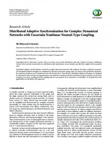
Figure 1: Values of the unknown bias.

0

20

FF2

the gyroscope as a measurement sensor is considered [26]. The spacecraft attitude tracking system, which is mainly used to enhance and track the spacecraft drift signal, is corrupted by the unknown bias. The corresponding discretetime dynamic stochastic system is expressed as 0 1 0.0129 0 ]x + [ ] p + [ ] w𝑘 , −0.85 1.70 𝑘 −1.2504 𝑘 1 z𝑘 = [0 1] x𝑘 + k𝑘 .

0.06 0.05

(39) 0.04

(40)

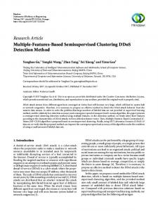
As in the literature [21], we assumed that x = [𝑥1, 𝑥2]𝑇 , w𝑘 ∼ 𝑁(0, 0.012 ), and k𝑘 ∼ 𝑁(0, 0.012 ). The true state x0 = [2, 1]𝑇 and the unknown bias p0 ∼ 𝑁(0, 0.52 ) were added to the dynamic equation (39). The initial estimates of the state ̂ 0 = 0. In simulation, the dynamic x̂0 = [1.8, 0.9]𝑇 , and bias p system is disturbed by some external disturbances, and the values of the unknown biases p𝑘 are plotted in Figure 1. The MAFSKF and SKF use Q𝑝 = 0.001 × 0.52 as the covariance of the bias p, which is one thousandth of the real covariance Q𝑝 = 0.52 . The constant 𝛽 in MAFSKF algorithm is set as 𝛽1 = 1 and 𝛽2 = 100, the softening factor 𝜀 is set as 𝜀 = 1, and the forgetting factor is 𝜌 = 0.95. Each single run lasts for 200 samples and 100 Monte Carlo runs are performed. The root mean squared errors (RMSE) of the state estimate are calculated to compare the performance of the MAFSKF algorithm and the SKF algorithm at each epoch. The simulation results are shown in Figures 2–5. Figure 2 shows the time evolution of the multiple fading factor in simulation. From Figure 2, we can see that the fading factors of the states become larger in order to recover the filter from divergence, and the second fading factor is greatly larger than the first one because the second state changes largely. Figures 3 and 4 show the RMSEs of the state estimates both 𝑥1 and 𝑥2 by using the conventional SKF and MAFSKF algorithm, respectively. The RMSEs of the MAFSKF algorithm on its own are given in Figure 5 to well show the results. From Figures 3 and 4, it is obviously seen that the MAFSKF algorithm can adapt these unknown biases and well track the true states, compared to the SKF. As

x1 RMSE

x𝑘+1 = [

Figure 2: Time evolution of the multiple fading factor.

0.03 0.02 0.01 0

0

20

40

60

80

100 120 Step

140

160

180

200

SKF MAFSKF

Figure 3: RMSE of 𝑥1 for 100 random simulation runs.

a result, the performance of the MAFSKF algorithm is better than the SKF when the information of the unknown biases is incomplete.

6. Conclusions In this paper, the multiple adaptive fading Schmidt-Kalman filter is presented to mitigate the negative effects of the unknown biases in dynamic or measurement model. In practice situations, the dynamic and measurement models include some additional unknown biases, which always bring greatly negative effects to the state estimates. Although the Schmidt-Kalman filter “considers” the biases, the uncertain initial values and incorrect covariance matrices of the unknown biases still are not considered. To solve the problem,


7

Acknowledgments

0.12

The work described in this paper was supported by the National Nature Science Foundation of China (Grant no. 11202011) and the Fundamental Research Funds for the Central Universities (Grant no. YWK13HK11). The authors fully appreciate the financial supports. The authors would also like to thank the reviewers and the editor for their many suggestions that helped improve this paper.

0.1

x2 RMSE

0.08 0.06 0.04

References

0.02 0

0

20

40

60

80

100 120 Step

140

160

180

200

SKF MAFSKF

x1 RMSE

Figure 4: RMSE of 𝑥2 for 100 random simulation runs. 0.03 0.025 0.02 0.015 0.01 0.005 0

0

20

40

60

80

100 120 Step

140

160

180

200

60

80

100 120 Step

140

160

180

200

MAFSKF ×10 12

−3

x2 RMSE

11 10 9 8 7

0

20

40

MAFSKF

Figure 5: RMSE for MAFSKF.

the MAFKF is proposed to adjust the covariance of the states and noise by using the multiple fading factors as a multiplier on the outside of the a priori covariance equation when the information about the dynamic or measurement model is incomplete. Then, the MAFSKF is designed based on the MAFKF. Numerical simulation shows that the MAFSKF can mitigate the negative effects of incorrect covariance matrices of the unknown biases compared to the SKF.

Conflict of Interests The authors declare that there is no conflict of interests regarding the publication of this paper.

[1] R. Lu, Y. Xu, and A. Xue, “𝐻∞ filtering for singular systems with communication delays,” Signal Processing, vol. 90, no. 4, pp. 1240–1248, 2010. [2] R. Lu, H. Li, A. Xue, J. Zheng, and Q. She, “Quantized 𝐻∞ filtering for different communication channels,” Circuits, Systems, and Signal Processing, vol. 31, no. 2, pp. 501–519, 2012. [3] A. Garulli, A. Vicino, and G. Zappa, “Conditional central algorithms for worst case set-membership identification and filtering,” IEEE Transactions on Automatic Control, vol. 45, no. 1, pp. 14–23, 2000. [4] S. F. Schmidt, “Application of state space methods to navigation problems,” in Advanced in Control Systems, pp. 293–340, Academic Press, New York, NY, USA, 1966. [5] D. Woodbury and J. Junkins, “On the consider Kalman filter,” in Proceedings of the AIAA Guidance, Navigation, and Control Conference, AIAA Paper 2010-7752, Toronto, Canada, 2010. [6] A. H. Jazwinski, Stochastic Processes and Filtering Theory, Academic Press, New York, NY, USA, 1970. [7] B. D. Tapley, B. E. Schutz, and G. H. Born, Statistical Orbit Determination, Academic Press, New York, NY, USA, 1st edition, 2004. [8] R. Zanetti and C. D. Souza, “Recursive implementations of the consider filter,” in Proceedings of the AAS Jer-Nan Juang Astrodynamics Symposium, College Station, Tex, USA, 2012. [9] G. J. Bierman, Factorization Methods for Discrete Sequential Estimation, Dover Publications, 2006. [10] D. P. Woodbury, M. Majji, and J. L. Junkins, “Considering measurement model parameter errors in static and dynamic systems,” Journal of the Astronautical Sciences, vol. 58, no. 3, pp. 461–478, 2011. [11] S. A. Chee and J. R. Forbes, “Norm-constrained consider Kalman filtering,” Journal of Guidance, Control, and Dynamics, vol. 37, no. 6, pp. 2048–2053, 2014. [12] Q. Xia, M. Rao, Y. Ying, and X. Shen, “Adaptive fading Kalman filter with an application,” Automatica, vol. 30, no. 8, pp. 1333– 1338, 1994. [13] C. Hide, T. Moore, and M. Smith, “Adaptive Kalman filtering for low-cost INS/GPS,” Journal of Navigation, vol. 56, no. 1, pp. 143–152, 2003. [14] C. Hu, W. Chen, Y. Chen, and D. Liu, “Adaptive Kalman filtering for vehicle navigation,” Journal of Global Positioning Systems, vol. 2, no. 1, pp. 42–47, 2003. [15] K. H. Kim, J. G. Lee, and C. G. Park, “Adaptive two-stage Kalman filter in the presence of unknown random bias,” International Journal of Adaptive Control and Signal Processing, vol. 20, no. 7, pp. 305–319, 2006. [16] D. H. Zhou, Y. G. Xi, and Z. J. Zhang, “A suboptimal multiple fading extended Kalman filter,” Acta Automatica Sinica, vol. 17, no. 6, pp. 689–695, 1991.

8 [17] Y. Geng and J. Wang, “Adaptive estimation of multiple fading factors in Kalman filter for navigation applications,” GPS Solutions, vol. 12, no. 4, pp. 273–279, 2008. [18] W. Gao, L. Miao, and M. Ni, “Multiple fading factors kalman filter for sins static alignment application,” Chinese Journal of Aeronautics, vol. 24, no. 4, pp. 476–483, 2011. [19] H. E. S¨oken and C. Hajiyev, “Adaptive unscented Kalman filter with multiple fading factors for pico satellite attitude estimation,” in Proceedings of the 4th International Conference on Recent Advances in Space Technologies (RAST ’09), pp. 541– 546, Istanbul, Turkey, June 2009. [20] D. L. Snyder, “Information processing for observed jump processes,” Information and Computation, vol. 22, no. 1, pp. 69– 78, 1973. [21] L. Ozbek and F. A. Aliev, “Comments on adaptive fading Kalman filter with an application,” Automatica, vol. 34, no. 12, pp. 1663–1664, 1998. [22] J. Deyst and C. F. Price, “Conditions for asymptotic stability of the discrete minimum-variance linear estimator,” IEEE Transactions on Automatic Control, vol. 13, pp. 702–705, 1968. [23] H. W. Sorenson and J. E. Sacks, “Recursive fading memory filtering,” Information Sciences, vol. 3, no. 2, pp. 101–119, 1971. [24] W. Qian, L. Wang, and Y. Sun, “Improved robust stability criteria for uncertain systems with time-varying delay,” Asian Journal of Control, vol. 13, no. 6, pp. 1043–1050, 2011. [25] J. L. Crassidis and J. L. Junkins, Optimal Estimation of Dynamic Systems, Chapman & Hall/CRC Press, Boca Raton, Fla, USA, 2nd edition, 2012. [26] P. S. Kim, “Separate-bias estimation scheme with diversely behaved biases,” IEEE Transactions on Aerospace and Electronic Systems, vol. 38, no. 1, pp. 333–339, 2002.


Advances in

Operations Research Hindawi Publishing Corporation http://www.hindawi.com

Volume 2014

Advances in

Decision Sciences Hindawi Publishing Corporation http://www.hindawi.com

Volume 2014

Journal of

Applied Mathematics

Algebra

Hindawi Publishing Corporation http://www.hindawi.com


Volume 2014

Journal of

Probability and Statistics Volume 2014

The Scientific World Journal Hindawi Publishing Corporation http://www.hindawi.com


Volume 2014

International Journal of

Differential Equations Hindawi Publishing Corporation http://www.hindawi.com

Volume 2014

Volume 2014

Submit your manuscripts at http://www.hindawi.com International Journal of

Advances in

Combinatorics Hindawi Publishing Corporation http://www.hindawi.com

Mathematical Physics Hindawi Publishing Corporation http://www.hindawi.com

Volume 2014

Journal of

Complex Analysis Hindawi Publishing Corporation http://www.hindawi.com

Volume 2014

International Journal of Mathematics and Mathematical Sciences


Journal of

Mathematics Hindawi Publishing Corporation http://www.hindawi.com

Volume 2014


Volume 2014

Volume 2014


Volume 2014

Discrete Mathematics

Journal of

Volume 2014


Discrete Dynamics in Nature and Society

Journal of

Function Spaces Hindawi Publishing Corporation http://www.hindawi.com

Abstract and Applied Analysis

Volume 2014


Volume 2014


Volume 2014

International Journal of

Journal of

Stochastic Analysis

Optimization



Volume 2014

Volume 2014