Everyone knows (don't they) that rich people and poor people live in different places. ... advice, and to Charles Lound of the Office for National Statistics for ...
Rich place, poor place: an analysis of geographical variations in household income within Britain1
Richard Berthoud Institute for Economic and Social Research University of Essex
The question Everyone knows (don’t they) that rich people and poor people live in different places. Compare standard images of the depressed north and the thriving south east. Or the stereotypes of Mayfair on the one hand and Hackney on the other. The idea of this clear social and economic segmentation dates back hundreds of years, and has often been used in fiction and in documentaries to illustrate the extremes of wealth and poverty. At a more formal level, geographers and policy makers have analysed the characteristics of prosperous and deprived areas. Seebohm Rowntree’s classical study of poverty in York in 1899 covered only the ‘working class’ areas of the town, on the assumption that no one was poor in other districts (Rowntree 1901). Over the past 25 years, there have been numerous attempts to classify areas in terms of some index of deprivation (eg Holterman 1975, Begg and Eversley 1986, Robson and Tye 1995, DETR 2000). Many policies have been formulated to deliver services to deprived areas - whether this is a global policy (such as the calculation of central government subsidies to local authorities) or a specific one (such as ‘Action Zones’ in health, education and housing). The government has recently announced a ‘national strategy for neighbourhood renewal’ which is based, at least in part, on the idea that ‘poor neighbourhoods’ play a substantial role in the causation of ‘poverty’ (SEU 2001). Nevertheless, the extent to which targeting areas is an effective way of focusing policy initiatives on those in greatest need has continually been questioned. In the mid-1970s, for example, the evaluation of Educational Priority Areas pointed out that most deprived children 1
This research was supported by the Nuffield Foundation. The FRS data which is the basis for most of the analysis was provided by the Department of Social Security. I am especially grateful to my former ISER colleague Vijay Verma for clarifying the procedure for estimating between-area variances (see Appendix 1); without his contribution I would have got the figures wrong. Thanks also to Nick Buck for his constructive advice, and to Charles Lound of the Office for National Statistics for explaining some details of the sample structure. None of these is responsible for the analysis, or the interpretation of the findings
did not live in deprived areas, while the majority of the children in such areas were not deprived (Barnes and Lucas 1975). Yet policy continues to adopt geographically-targeted approaches, perhaps in the absence of any other way of reaching the poor. It is important to distinguish in principle between the characteristics of an area itself, and the aggregate characteristics of the people who live there. An area is by the sea; in the North; near a coal field. These are intrinsic geographical facts. Its economy has been heavily dependent on an industry which is now in decline; it is poorly linked to the main road network; there is no hospital. These are all economic characteristics of the area. They could be changed by policy, but both the problem and the potential solution will be experienced by the area and its population as a whole. Places can be classified unambiguously in terms of these characteristics. Classifying areas in terms of the composition of their population is different. This area has a high proportion of pensioners; that area a high proportion of people with above-average incomes. Does that make the areas ‘old’ or ‘rich’? In some senses it may do so: the first place may be an appropriate place to set up a shop selling zimmer frames; the second may have high local tax yields and generously-endowed public services. All the people in the area might be affected in some way by the composition of its population - house values may rise, for example, following an influx of rich people. But in another sense they are not affected: the individuals who do not share the alleged common characteristic are not older and do not have more income than they would if they lived anywhere else. Indeed, they may feel the opposite of these characteristics, in comparison with their neighbours. The question always has to be asked - what is the extent of the polarisation which is being summarised when we classify areas by the composition of their populations? A clear example focuses on ethnic minorities. In parts of America, ‘ghettos’ have been defined strictly as places where almost all the people are black, and where almost all of the black population live (Duncan and Duncan 1950). In Britain, it is well known both academically and in popular discussion that there are high concentrations of black and Asian people. But there are no ‘ghettos’ here, as just defined (Peach 1996, Dorsett 1998), and only two local authority districts have members of minority groups constituting as many as half of their populations.2 This paper focuses on the distribution of household income between areas in Great Britain. The distribution of income between households has been studied in great detail, providing good measures both of inequality and of poverty (Goodman and others 1997, Jarvis and Jenkins 1998, DSS 1998). But how much of the inequality in incomes should be accounted for by variations between regions, between towns or between neighbourhoods. What proportion of ‘poor’ households can be found in ‘poor’ places? Measuring area variations Most of the many attempts to classify local areas in Britain have been based either on the Census alone, or on a combination of the Census and of administrative data derived from social security transactions, the delivery of health services or the activities of local government agencies. The deprivation index currently used by the Department of the Environment, Transport and the Regions as the basis for determining grant aid to local 2
About 60 per cent of the populations of the London Boroughs of Brent and Newham are from ethnic minorities, according to the Labour Force Survey.
authorities, for instance, takes account of 32 items of information under six headings (DETR 2000): income (ie social security benefits); employment; health deprivation and disability; education, skills and training; housing; geographical access to services. The aim of indices such as the DETR’s is to classify all areas, or to identify all deprived areas, so that resources and/or policies can be targeted as intended. For this purpose, the data sources must have two features: they have to be available about all areas, and they have to be accurate about each area, at the required level of spatial disaggregation. Both of these conditions are achieved by the Census, though that is at the end of its ten-year cycle usefulness just now. Some kinds of administrative data are now collected in such a way that they can be analysed at quite a fine grain of local areas, though other elements are available only at, say, the local authority level. For research and analytical purposes, however, it is not necessary to provide complete coverage in this way. If instead of asking ‘which specific areas are the most deprived?’ we asked ‘how much variation is there between areas?’ or ‘what type of area tends to be deprived?’, full coverage is not essential. A sample of areas is sufficient; and data about a sample of individuals or households may be adequate within each area analysed; provided always that the number of areas, and the number of cases within each area, are large enough to minimise sampling error. The use of sample data to draw general conclusions about geographical inequalities will be discussed in more detail later in this paper. Another feature of most analysis in this field is the combination of a fairly large number of different variables into an ‘index’ of deprivation rather than a single clearly-defined ‘measure’. A strong argument in favour of such an approach is that there is no single clearly defined concept of deprivation, and that the combination of a large number of indicators is the most appropriate way of getting at a nebulous underlying concept. The parallel is with the use of 20 or 30 questions in an examination to measure competence at mathematics, rather than a single test question which could not represent all facets of the subject. In the more sophisticated deprivation exercises, complex factor and/or cluster analyses are used to identify the key variables, and to distinguish different types of area (Folwell 1993). On the other hand, many of these indices are interpreted, directly or indirectly, as though they were indicators of ‘poverty’, a concept clearly related to levels of household income. The multivariate approach may be seen as a substitute for the key variable, income, which is not available in the Census or from any other source. At the least, it could be argued, income should be one of the contributors to the analysis, if that were possible. The use of multivariate indices of area variation also tends to confuse discussion of the relative importance of variations between areas and variations between the people within areas. The area index does not classify each of the people, so measures of individual variation between them are not a natural output from the analysis. Nevertheless, some work has been undertaken which questions the assumption - known as the ‘ecological fallacy’ - that area effects provide a significant explanation of the experiences of individuals, or that most
‘deprived’ people live in ‘deprived’ areas (Cullingford and Openshaw 1979, Fieldhouse and Tye 1996). These various considerations all point to the desirability of the analysis of geographical variations in the distribution of household income. Income provides the single measure which is most closely associated with the concept of poverty. The distribution of income between households is a major subject of research in its own right, and the analysis of geographical inequalities should form part of that body of research. At the same time, the use of this welldefined household-level variable can contribute substantially to the study of geographical inequalities. Since the British Census does not include an income question (unlike its American counterpart), analysis of the spatial distribution of income has been seriously hampered by lack of data. The DETR index (referred to above) includes Income Support and other social security payments; these may provide good proxy measures of low income, but clearly make no distinction between households with medium and high incomes. Nearly 25 years ago I undertook an analysis of the distribution of income within London, based on a crude income question included in the very large sample of households taking part in the 1971 Greater London Transportation Study (Berthoud 1976). A major step forward was achieved in the mid 1990s, with the development of the Family Resources Survey. This annual enquiry, described in the next section, provides the basis for the first accurate assessment of the relative importance of area variations in the distribution of income in Great Britain. As a sample survey, it does not tell us which specific areas are rich and which are poor, though a brief discussion of how it might contribute to that objective is offered at the end of this article. What it does do is show how far the difference between rich and poor people can be characterised in terms of rich and poor places.
The Family Resources Survey The FRS has been undertaken under the auspices of the Department of Social Security since 1993. It collects detailed income data from each member of 25,000 households annually. The data analysed here are from 1994/95 and 1995/96.3 The structure of the FRS sample is crucial to this analysis. It is similar to the majority of large scale national surveys conducted in Britain. The following is a direct extract from the official report on the 1995/96 survey (DSS 1997). The FRS uses a stratified clustered probability sample drawn from the Office for National Statistics’ small users postcode address file (PAF). The PAF is a list of all addresses where less than 50 items of mail are received a day, and is updated twice per year. The survey selects 1752 postcode sectors4 with a probability of selection which is proportional to size. Each sector is known as a Primary Sampling Unit (PSU).
3
An FRS ‘year’ is defined as April through March. An annual survey is therefore characterised as (eg) 1994/95.
The PSUs are stratified by 24 regions5 and three other variables. Stratifying ensures that the proportion of the sample falling into each group reflects those of the population. Within each region, the postcode sectors are then ranked and grouped into six equal bands using the proportion of heads of household in socio-economic groups 1 to 5 and 13. Within each of these six bands, the PSUs are ranked by the total unemployment rate and formed into three further bands, resulting in 18 bands. These are then ranked according to the proportion of households that are owner-occupied. The set of stratifiers is chosen to have a maximum effectiveness on the accuracy of two key variables: household incomes and housing costs. Within each PSU a sample of addresses is selected. The 1995-96 average was 24 addresses per PSU. Each year, one half of the PSUs are retained from the previous year’s sample; while for the other half of the sample, a fresh selection of PSUs is made (which in turn will be retained for the following year). This is to improve comparability between years. The original sample chosen for 1995-96 consisted of 1752 x 24 = 42,048 addresses. Interviewers established that 5,494 were ineligible because they were not private households; but an additional 1,148 households were identified because of multi-occupancy. Of the effective sample of 37,712 households, 26,435 provided complete data about each household member and are available for analysis, a net response rate of 70 per cent. Very similar returns were recorded in 1994/95. Thus the key features of each year’s FRS sample are: • a random sample of 1752 postcode sectors; and • a random sample of (an average of) 15 households within each sector (26,435 ÷ 1,752). When two consecutive years of FRS data are combined, the fact that half the PSUs are repeated from one year to the next gives us: 876 two-year sectors with an average of 30 respondent households each, plus 1752 single-year sectors with an average of 15 households. The detailed distribution of the number of interviews per sampling point is shown in Table 1. The number ranged from 0 to 44. The mean was just under 20, but the combination of twoyear and one-year sectors gives a bimodal distribution with peaks at 15 and 29.
4
British postal zones are coded in a hierarchical format. If we take the single best-known code, the House of Commons is SW1A 1AA. The postcode sector is identified by the numeric characters following the space (SW1A 1). Another example is the University of Essex, whose full postcode is CO4 3SQ; the sector is CO4 3. 5 The ‘regions’ used were: 17 in England (metropolitan/non-metropolitan/4 in London); 2 in Wales; 5 in Scotland. No sample was selected in Scotland north of the Caledonian Canal, an area of very low density of population which accounts for 0.25% of the population of Great Britain. Northern Ireland is not included in the survey; it is known to have much the lowest incomes of any region of the UK (Cabinet Office 1999).
Table 1 Number of household interviews achieved in each selected sector Number of interviews
Number of sectors
0-4
10
5-9
92
10-14
714
15-19
858
20-24
213
25-29
286
30-34
303
35-39
138
40-44
12
There are approximately 9,200 postcode sectors in Great Britain. Since there were about 23,700,000 households in the mid-1990s, that means that each sector contained, on average, 2,500 households. The average local authority district includes 19 postcode sectors. Thus the primary geographical analysis in the FRS was comparable in size to, but rather smaller than, an electoral ward, which contained, on average, 2,800 households. It is substantially larger than the Census enumeration district (ED) which averages only 200 households.
Analytical approach The FRS contains data about a large and representative sample of small areas, though only a small sample of households within each area. It is not possible to use these data to estimate the mean income, or any other statistic, within each specific area. This is for two reasons. First, the data available to independent analysts does not record where the area was. We know that these 20 households lived in one sector, and those 20 lived in some other sector, but we know no more than that, apart from the name of the local authority district within which the sector lay. Second, a sample of 20 is not sufficient to estimate income statistics with any accuracy. For example, the error on the estimate of the mean income in an average 20household PSU was ±£66 per week (using 95 per cent confidence intervals), on an overall mean of £259. What we can do, though, is to estimate general statistics about variations between and within sectors. The overall variance in the distribution of household income is calculated as the sum of the squares of the difference between each household’s observation and the overall average. This can be split into two components: the difference between each household’s observation and the average for its sector; and the difference between the sector average and the national average. The overall variance then equals the sum of the within variances and the between variances: Total variance = Within sector variance + Between sector variance When the data within each sector are based on a sample (rather than on information about the whole population), it is not possible to calculate the within- and between-sector variances
directly. But the statistical procedure known as analysis of variance provides an estimate of the ratio between the two. The calculations are discussed in an Appendix to this paper. Note that although the estimates of the average income and the variance for each specific sector are subject to the large sampling error associated with samples of only about 20 households, the analysis of the overall distribution of within- and between-sector variances is not. These are statistics about the population which are just as accurate as the estimate of the mean. Since we have samples of 50,000 households in 2,600 sampling points, this means that the estimates are very accurate indeed.
Treatment of income The FRS involves an interview with each adult member of the household. Details are collected about the amounts of every source of income received by each person: earnings, social security benefits, pensions and investment income. A total has been calculated for the household. Housing costs were not subtracted. For most of the analysis in this paper, household income is expressed in ‘equivalent’ terms: the total is divided by a factor based on the number of people in the household and their ages to provide a measure of income in relation to needs which is similar in concept to an ‘income per head’. The data and the conventions for analysing it are exactly the same as are used by the Department of Social Security for its annual analysis of Households Below Average Income (DSS 1998), with some exceptions explained in the following paragraphs. The analysis here counts each household as a unit, although the DSS weights by the number of adults and children in the household to produce estimates of the number of individuals in each income band. All money amounts from the 1994/95 survey have been inflated by 4.2 per cent to represent the average difference between the two survey years. This eliminates a spurious source of variation between the 1994/95 sectors and the 1995/96 sectors. The distribution of household income recorded by the FRS has been truncated at both ends. 332 households, 0.6 per cent of the whole sample, were reported to have a net income less than zero. That is, their taxes exceeded the sum of their earnings, benefits and other resources. We can be sure that this is not a true estimate of the household’s command over resources. Moreover, these households with negative incomes were no more common in sectors where there were, otherwise, a large number of low-income households. So it has to be assumed that there has been some sort of misreporting in the data, which will exaggerate the level of within-sector variance. By the same token, households who reported a net equivalent income in excess of £1,000 per week (£52,000 per year) have also been excluded. There were 497 cases, 1.0 per cent of the original sample. Such large incomes are not logically impossible in the same way as negative incomes. But it is clear that very high incomes are poorly captured by social surveys. The DSS HBAI analysis deals with this by weighting the high-income households by factors designed to match the distribution of high incomes recorded by the Inland Revenue (DSS 1998). But weighting small numbers of households in that way would have had serious effects on our estimates of between-sector variances. At least some of those observed may have been transcription errors (eg recording £200.00 as £20,000) The cases excluded were
slightly more common in sectors which appeared (from the remaining cases) to have aboveaverage incomes, than in low-income sectors, but this association was much less strong than it ‘ought’ to have been if all the high reports of income were true. Because the variance statistics used in this analysis are based on the square of incomes, the small number of very high-income households had a huge effect on the analysis. In common with Goodman, Johnson and Webb (1997), all households in the top 1 per cent of the distribution of income have therefore been omitted. The effect of both these income truncations was to reduce the apparent level of inequality within postcode sectors, and so to increase the estimate of the geographical dispersion between sectors. Between-sector differences accounted for 5.4 per cent of overall variance when all incomes were included. The estimate rose to 6.1 per cent when the negative incomes were dropped. It rose again to 9.8 per cent when the top one per cent of incomes were also dropped. In a sense, the truncation has been justified by the outcome: the negative and very high incomes were not well associated with the geographical distribution of the remainder of incomes, and including them would have led to an under-estimate of the true geographical effect. The main argument of this article is that the effect is small; it would be even smaller if the outliers were added back in.
Income variations between households, and between sectors Figure 1 plots the distribution of equivalent income measured first for each household, and then for each postcode sector, taking the average of the households in each sector.6 Household incomes had the distribution which is familiar to income analysis, a ‘skewed normal’ distribution with a high peak rather below the mean, and a long tail of small numbers of households with incomes well above the mean. It is immediately clear that the distribution of the average incomes of sectors was much narrower, with a high peak close to the overall average, and relatively few cases much below or above average. Figure 1 Distributions of the equivalent weekly income of households and of the average incomes of sectors 10000 Households Sectors
8000 6000 4000 2000 0 0
200
400
600
800
1000
Note: vertical axis counts the number of households in £25 income ranges (£0-£24.99, £25-£49.99 etc) 6
For ease of comparison between the two levels of measurement, all sector-level statistics have been based on the number of households interviewed in each sector. Thus, the statement that (for example) ‘x per cent of sectors had an average income of less than £y per week’ should strictly be read as ‘x per cent of households lived in sectors which had an average income of less than £y per week.’
It is statistically inevitable that the distribution of area incomes is narrower than the distribution of individual incomes, if the area figures are the means of the individual figures. That is, if there is any variation at all within each area, the variation between areas is necessarily reduced, compared with the full distribution. The question at issue is the extent of this difference between the two levels of measurement. The same distributions are shown in Table 2 in broad bands chosen to illustrate the differences between households and sectors. Nearly a quarter of all households reported an equivalent income of up to £150 per week. Hardly any postcode sectors had an average income as low as that. At the opposite end of the scale, one tenth of households, but again hardly any sectors, enjoyed equivalent incomes above £450 per week (but lower than the cutoff point, described earlier, of £1,000 per week). In fact nearly three quarters of sectors were bunched into the middle range of average incomes, between £200 and £325 per week. Table 2 Distribution of household and sector equivalent incomes in broad bands Households
Column percentages Sectors
Up to £150 per week
23
0.3
£150-£200
21
13
£200-£325
31
75
£325-£450
15
11
£450-£1000
10
0.4
These findings strongly suggest that the range of inequality of household incomes within post-code sectors was substantially larger than the range of between sector averages. This leads to the central summary statistic of this analysis - already quoted - that between-sector variations accounted for only 9.8 per cent of overall variations in household incomes. An interpretation of this statistic is that if we were trying to guess how much income a particular household received, we would be only 9.8 per cent more accurate if we knew which sector the household lived in, than if we had no knowledge of its whereabouts. Remember, that this analysis is based on quite small geographical units - sectors averaging only 2,500 households each. The analysis shows that there is a significant concentration of incomes in particular areas - on such a large sample, there is no doubt of that. We can reject overwhelmingly the hypothesis that there is no difference between areas. On the other hand, the hypothesis that all the incomes in any sector are the same, has to be rejected even more emphatically. It is doubtful whether the extent of concentration – just under 10 per cent accounted for by small residential areas - is sufficient to confirm the popular assumptions about polarisation discussed earlier, or endorse the use of area-based policies to reach ‘poor’ (or ‘rich’) people. Those issues are discussed in more detail in the concluding section.
Alternative measures of income All the analysis so far has been based on the definitions most commonly adopted in analysis of the British income distribution. The side-headings in Table 3 summarise the differences between six commonly used alternative measures of income (all calculated for whole households), and the first column gives the overall averages to illustrate the differences between the concepts. Earnings contribute by the far the largest proportion of the national income. They are also the most unequally distributed between households, mainly because many households have no earnings, but do receive occupational pensions and/or social security benefits instead. The differences between the alternative measures’ overall levels of inequality, as measured by the coefficients of variation in Table 3, are all predictable and well-known.7 It is not so easy, though, to predict how each component of income would be distributed geographically. Of course, taxes will tend to reduce the income in prosperous areas, and benefits will raise the incomes in deprived areas, but they also reduce inequality between households. Table 3 Percentage of income variation explained by between-sector differences: six measures of household income Measure of income
Average
Coefficient of variation between households8
Between-sector explanation of variance
Earnings
£246
1.22
7.1%
+ occupational pensions, investment income etc
+£39
Market income
£285
1.05
9.8%
0.77
9.1%
0.69
8.1%
0.57
9.8%
0.66
8.5%
+ social security benefits Gross income - direct taxes Net income ÷ equivalence scale Equivalent income before housing costs - housing costs Equivalent income after housing costs
+£65 £350 -£76 £274 ÷1.06 £259 -£41 £218
It turns out that all the measures of income produced broadly similar results, with betweensector differences explaining between 7.1 and 9.8 per cent of inequality. Earnings were least concentrated geographically - this may be a surprising finding, suggesting that the location of high and low paid jobs is not the most important influence on the overall pattern. Market income (the combination of earnings and other non-state sources) was one of the most concentrated. Equivalent income before housing costs - the standard measure used in all the other sections of this analysis - had a relatively low level of overall inequality, but a high 7
Though all, are, of course, affected by the truncation of negative and high values described earlier. The truncation was undertaken for all cases on the basis of equivalent income before housing costs, rather than separately for each measure of income. 8 The coefficient of variation is calculated as the standard deviation divided by the mean. It can be interpreted as a measure of inequality between households.
degree of geographical dispersion. The combination of those two factors means that withinsector variations were lower on this measure than on any other.
Rich and poor households in rich and poor places The main policy objectives of analyses of area variations in prosperity and poverty are concerned with targeting. Commercial organisations might want to identify better-off areas in order to aim sales campaigns at people with the greatest spending power. National and local government often want to identify worse-off areas in order to focus service provision on people with the greatest needs. Political parties want to locate the voters most likely to support their causes. Of course the current analysis does not provide measures of the income of specific areas anyway, but if it was possible to identify the sectors with high and low incomes accurately, how efficiently could this information be used to reach households with high and low incomes? In recent years ‘poor’ households have usually been defined as those whose equivalent income is below half the national average. 15 per cent of households in the FRS were poor on that definition. But it is convenient for the present analysis to allocate the labels ‘well-off’ and ‘poor’ on the basis of the quintiles of the distribution: that is, the highest 20 per cent of incomes (with equivalent incomes above £357 per week) and the lowest 20 per cent (below £143 per week). Given what has already been shown about the relative width of the distributions, it is no surprise to find that hardly any postcode sectors had an average income above £357 or below £143; just 1 per cent would have been called ‘poor’ on that criterion, and 2 per cent ‘well off’.9 But there were, of course, sectors which recorded relatively high or low average incomes, and they have also been divided into five equal groups, labelled in purely relative terms from ‘lowest income’ to ‘highest income’. Since the groupings of both household incomes and sector incomes have been based on the quintiles of their distributions, measures of concentration can be interpreted rather simply. In the logically extreme case where there was no concentration, the proportion of poor households in every type of sector would be 20 per cent; and 20 per cent of all poor households would be found in each type of sector. At the opposite extreme, if households were entirely segregated into sectors with others of the same income, all the residents of the lowest income areas would be poor, and all the poor would live in those sectors. Conversely the highest income areas would have collected all the better-off households. The symmetry of the definitions means that the measure of the risk of poverty/wealth and the measure of the share were identical.
9
Classification of sectors by average income has been based on the log of income, as the straight arithmetic mean tends to place more weight on the upper than the lower end of the distribution. Sectors with fewer than 10 household interviews have been excluded.
Table 4 Concentration of well-off and poor households in high and low income sectors Cell percentages Well-off households
Poor households Lowest income sectors
31
5
Below average
23
12
Average
20
18
Above average
15
25
Highest income sectors
11
40
Note: categories are based on quintiles of the distribution of incomes between households and between sectors, as described in the text. The percentages show that (for example): 31 per cent of the households in lowest income sectors were poor; and also that 31 per cent of poor households lived in the lowest income sectors
Figure 2 Concentration of well-off and poor households in high and low income sectors
Rich
Highest
Above average
Average
Middle income
Below average
Poor
Lowest
0%
20%
40%
60%
80%
100%
The extent of concentration is shown in Table 4 and Figure 2. About a third of the households in the lowest fifth of all sectors were poor; and these represented about a third of all poor households. The risk and share of poverty in the highest income sectors was 11 per cent. Thus there were real variations in the composition of high and low income areas. But they were not strong enough to locate poor households very efficiently. In fact the concentration of betteroff households was slightly stronger: the risk/share in the highest income areas was 40 per cent, and only 5 per cent in the lowest income sectors. In neither case is it possible to say that the majority of poor/well-off households lived in the lowest/highest income sectors; or that they constituted a majority of the population of such areas.
Alternative levels of geographical aggregation Analysis of geographical variations depends very much on the grain of the analysis. At the extremes, treating the whole of Britain as a single area will explain none of the variation in income; dividing the country into 24 million areas each containing one household will explain all the variation. The geographical unit on which the FRS sample is based - the postcode sector - contains an average of 2,500 households. A finer grain would explain more variation, a coarser grain would explain less.10 It is also important to consider what processes might be at work in social segregation at different levels of analysis. It seems likely that variations in incomes between areas which are a long way apart will be mainly economic. London has many jobs in thriving industries; Newcastle has few jobs, mainly in declining industries. Such differences in regional economies would impose variations between the areas in the incomes of people living there; modified in part by a tendency for people to migrate from the poorer to the wealthier area. In contrast, variations in incomes between areas which are close together will mainly arise from residential sorting. The residents of Mayfair and Hackney are probably all within daily travelling distance of a similar range of jobs. Those who secure the best jobs choose to live in areas with large houses, a pleasant environment and social cachet; and prices are correspondingly high. Those with no job, or low-paid jobs, are obliged to live in areas with less well-endowed properties, dirty streets and a ‘rough’ neighbourhood. Thus the processes behind income segregation are probably quite distinct, depending on the distance between areas. This is related to, though not the same as, the coarseness of the grain of the analysis. It may also vary according to the size of the settlement: a postcode sector may represent the whole of a village in a rural area, with its own mixture of rich and poor, while one sector is a tiny fraction of the population of a large city, and offers, perhaps, more opportunity for polarisation. The largest geographical division in Great Britain is the region, of which there are ten. It is not unusual to show London separately from the rest of the South East, and that principle has been extended in Table 5 to distinguish each of the eight conurbations from the region of which they are normally a part, to make a total of 18 units. The design of the FRS sample is such that there are substantial numbers of postcode sectors (PSUs) in each region, and this (rather than the number of households interviewed) is what determines the accuracy of the regional estimates. The striking thing about the distribution is its uniformity. A stereotype was suggested at the beginning of this article of the depressed North East and the prosperous South East. The bestoff and the worst-off regions were indeed the South East on the one hand and South Yorkshire (greater Sheffield) and Tyneside (greater Newcastle) on the other. The range of average incomes between these - £293 to £224 - can be restated as about one quarter of the overall average. In general, regions with low average incomes had high proportions of households in poverty (defined, as before, as the lowest fifth of incomes): the range here was between 15 per cent in the South East and 26 per cent in South Yorkshire. But, given the full range of 18 regions between the best and the worst off, the variation in household incomes is 10
It is not clear how far the boundaries of post-code sectors are drawn along natural social or structural divisions to form meaningful ‘neighbourhoods’, and how far just as lines on the map.
not great. In fact differences between regions (as defined here) accounted for just 2.7 per cent of the overall inequality in household incomes. The figures in Table 5 are based on household income before housing costs. In fact rents and mortgage payments are higher in London and the South East than elsewhere, and these can be interpreted as offsetting the variations in total income. If income after housing costs is used as the measure of prosperity, the proportion of variance explained by the regional analysis falls to only 1.5 per cent.
Table 5 Equivalent household incomes by conurbation and region Average income
Percent of households who were poor
Percent of sectors which were lowest income
Number of sectors in sample
London
£287
17%
10%
321
South East (best)
£293
15%
5%
504
South West
£256
19%
15%
225
East Anglia
£261
20%
16%
99
East Midlands
£251
20%
20%
187
West Midlands (conurb)
£239
22%
35%
118
West Midlands (region)
£259
19%
14%
119
Merseyside
£234
24%
41%
63
Greater Manchester
£242
22%
31%
125
North West
£253
20%
21%
109
West Yorkshire
£240
23%
24%
94
South Yorkshire (worst)
£224
26%
43%
62
Yorks and Humberside
£242
22%
21%
77
Tyneside
£228
25%
45%
54
North
£234
22%
28%
94
Wales
£228
25%
34%
133
Greater Glasgow
£229
25%
34%
82
Scotland
£249
22%
21%
158
Note: Places in bold type are conurbations. In England, these are the metropolitan counties. Greater Glasgow is defined as Glasgow City, plus the districts directly bordering it. Places in ordinary type are regions, excluding the conurbations within them.
Remember that postcode sectors accounted for 9.8 per cent of income inequality. It is possible to record what proportion of sector variation could be explained by regional differences - 2.7 expressed as a proportion of 9.8 is 28 per cent. Thus regional variations in sector incomes were more important than sector variations in household incomes.
The variations between regions in the number of relatively low income sectors (the lowest fifth of sector incomes) was much wider than the variation in the number of poor households (Table 5). The poorest region had less than twice as many poor households as the richest; but it had more than eight times as many low-income sectors (43 compared with 5 per cent). This is a natural consequence of nesting the variance at successive levels of spatial analysis, but it also leads to an important interpretative point. Comparing regions according to the number of poor (or deprived) sectors will tend to exaggerate the differences between one part of the country and another, compared with a ‘true’ measure based on poor or deprived households. The Prime Minister’s line is that there is no North/South divide in Britain – there may be differences between regions, but variations between towns and neighbourhoods within regions are just as important. The income analysis suggests that such regional differences as do exist do follow a broad north/south pattern. And London, which shows up quite badly on some deprivation indicators, is shown to be one of the best-off regions on the income measure. Regional variation accounts for about a quarter of inequality between sectors. Sector analysis tends to exaggerate the regional picture. North/South can scarcely be interpreted as a defining characteristic when the full range of regional inequality accounts for only 2.7 per cent of household inequality. Preliminary findings from a similar analysis of data for the European Union suggest that regional variations in the UK are substantially narrower than those observed in the other large countries. In Italy, regional factors account for 10.9 per cent of household variation – more than is accounted for by postal sectors within Britain.11 Germany exhibits an equally wide range of variation, largely accounted for by the cleavage between the former West and East states. A similar analysis can compare variations in income between local authority districts,12 which provide a geographical unit in-between region and postcode sector.13 Differences between districts are illustrated in Table 6 using the seven metropolitan boroughs which make up the West Midlands conurbation. Average household income ranged from £218 per week in Sandwell to £238 in Coventry, except that Solihull was much higher than any of the others at £290 per week. Households’ risk of poverty could be as low as 14 per cent or as high as 28 per cent, while the number of low income sectors again ranged more widely, between 17 per cent and 49 per cent. On this occasion, it was not the same districts which appeared best or worst off on each measure, suggesting some interesting micro-patterns of greater or lesser polarisation within different districts.
11
It is hoped to complete an analysis of data from the European Community Household Panel (ECHP) in the course of 2001. Watch www.iser.essex.ac.uk/epag for details. 12 The word district is used here in its formal meaning as the geographical unit of local government, rather in its less precise sense of ‘part of town’. There are 489 districts in Britain, ranging in size from Birmingham (400,000 households) to the Isles of Scilly (700). Large districts each contributed many sectors (PSUs) to the FRS sample; small districts would have contributed one sector among several districts. 13 Districts are an exact sub-division of regions. Postcode sectors, which are based on a different classification system, are not exact sub-divisions of districts: a few straddle district boundaries.
Table 6 Equivalent household incomes by district within the West Midlands conurbation Average income
Percent of households Percent of sectors who were poor which were lowest income
Number of sectors in sample
Birmingham
£224
28%
47%
40
Coventry
£238
23%
49%
15
Dudley
£222
20%
17%
8
Sandwell
£218
24%
32%
12
Solihull
£290
14%
19%
16
Walsall
£237
19%
17%
14
Wolverhampton
£235
22%
35%
9
The general point, though, is that variations between districts were stronger than between regions, but weaker than between postcode sectors. Over the country as a whole, the highest average equivalent income was recorded in Richmond upon Thames, at £384 per week. The lowest was in Kingston upon Hull, which averaged only £200 per week. According to the formal measure used throughout this article, district inequality accounted for 5.7 per cent of the overall variation between households. As the summary in Table 7 shows, this means that districts accounted for more than half of the observed variation between sectors. Table 7 Explanation of income variances at successive levels of aggregation Percentages as a proportion of variation between . . Districts
Sectors
Households
47
28
2.7
58
5.7
variation between . . . Regions Districts Sector
9.8
Note: the table should be read as follows: 47 per cent of variation between districts is accounted for by variation between regions, and so on.
It may be argued that although between-sector differences accounted for only 10 per cent of income inequality, the measure of polarisation would increase steeply if smaller areas could be analysed. This argument suggests that the real differences are at street level rather than between units of 2,500 households. Although the FRS has no unit of analysis smaller than the sector, Figure 3 bases estimates of the degree of inequality between smaller geographical areas on the measures already given for regions, district and sector - the final column of Table 7. If the percentage of variation explained is plotted against the number of geographical units at each level in the country (both on log scales) the relationship seems to be sufficiently regular to suggest a pattern, even though it is based on only three observations. The top-right corner of the chart is defined by
the logic that the explanation of variance must reach 100 per cent if all 24 million households in the country were considered an ‘area’ in their own right. If a direct line is drawn between the sector figure and that extreme point, it can be estimated that enumeration districts (EDs), of which there are 120,000 in Britain, would account for 21 per cent of household income inequality. The graph can also be used to estimate roughly how many geographical units the country would have to be divided into, to account for as much as half (50 per cent) of the variance in household incomes. The answer, subject of course to the crudeness of the interpolation, is about 2.3 million areas. Thus it is not until the analyst can identify areas averaging only 10 households each, that as much as half the variation can be attributed to a tendency for people with similar incomes to live near each other.
Figure 3 Relationship between area inequalities and number of spatial units analysed Percentage of variance explained (log scale)
100 50% of variance ED
10
Sector District Region
1 1
100
10,000
1,000,000 100,000,0 00
Number of units (log scale) Note: solid line based on three observations; dashed line based on interpolation
Conclusions The idea that rich and poor are segregated into different residential areas is deeply imbedded in the popular imagination, in the distribution of commercial outlets and in the provision of public services. The Family Resources Survey has provided an important opportunity to analyse the extent of that segregation. Because it is a sample survey, it does not identify specific rich or poor areas, but it does offer an analysis of the geographical element in inequality of household incomes. The main finding of the analysis is that just under 10 per cent of the overall variation in household incomes can be accounted for by differences between postcode sectors. If the labels well-off and poor are attached to the top and bottom fifths of the distribution of household incomes respectively, there are virtually no sectors whose average incomes would place them in those categories. Even if sectors are divided in five groups according to the distribution of their average incomes, only 40 per cent of households in the highest income areas were ‘well-off’, and only 31 per cent of households in the lowest income areas were ‘poor’.
Should we conclude that the contribution of sector variations to income inequality is ‘only’ 10 per cent, or ‘as much as’ 10 per cent? The figures reported on the basis of the FRS show that there is a real area effect. Nevertheless, the variation between places seems much less than might have been expected on the basis of popular stereotype, and much less than has been assumed in the development of area-based social policies. The FRS data is highly accurate for this kind of analysis. The main technical problem is that the conclusion is sensitive to outliers in the household income distribution which may have been affected by measurement error. Most of the statistics in this paper are based on a truncated distribution, in which equivalent incomes below zero or above £1,000 per week have been omitted. If the low and high values were included, the geographical variations would have appeared much lower. The estimates here can be interpreted as maximum values. It stands to reason that between-area variations will be lower if a coarser grain of geographical units is analysed. Regions accounted for only 2.7 per cent of variations in income; local authority districts accounted for 5.7 per cent. By extension, the grain of analysis would have to be very fine indeed before spatial patterns accounted for a large proportion of income inequality. The country would have to be divided into more than two million neighbourhoods averaging only ten households each before as much as half the variance could be explained. This has been a descriptive analysis which has offered few clues about the processes involved in segregation. It seems likely that income variations between settlements which are distant from each other are caused by the economic position of the settlements - people are relatively rich or poor because they live in one settlement rather than another. But variations within settlements are probably caused by residential choices within a fixed pattern of economic prosperity - the area has relatively a high or low income because rich or poor people live there. One possibility was that different types of well-off people or different types of poor people would be more or less concentrated into high and low income areas than others. But other analyses (not shown in detail) suggested that poor pensioners, poor disabled people, poor lone parents and poor unemployed people were all very similar in their tendency to live in low income areas. A more interesting clue was provided by data about housing tenure, housing expenditure and house values. Accommodation is a characteristic which is often measured at the household level, but is clearly lodged within areas, and stays behind if the household moves. Figure 4 shows that the values of properties in low income postcode sectors were substantially lower (as measured by Council Tax bands) than in high income sectors. The role of housing as a mediator in income segregation would repay much more detailed investigation, but is beyond the scope of the present paper.
Figure 4 Council Tax band of households in high and low income sectors 100% EFG&H
80% 60%
C B
40% 20% 0% Lowest incomes
Below average
Average
Above average
Highest incomes
The underlying question for public policy is whether the inequality observed between areas is a useful way of reaching low-income households with their high levels of social need. The equivalent question for commercial organisations is the opposite: can areas be used as means of targeting high-income households with their high spending power? But the issues are discussed here in terms of targeting low-income households. They really need to be split in two. First, how can districts with an above-average proportion of low-income households be identified? Second, how fine a grain of analysis is required to pin-point poor households with any efficiency? Districts are the natural unit of coarse-grain analysis in Britain. They are the locus of local government - the more so as the two-tier administration within counties is being replaced by unitary authorities. The boundaries are intended to be set to allow people with common interests to elect local councils which will reflect those interests; though another consideration has been to ensure that the every authority should have a reasonable tax base. The deprivation index used by the DETR is specifically designed as the basis for allocating central government subsidies. In this case, the identification of poor authorities is an object in its own right, not merely a device for identifying poor households. There is not a great range of income variation between districts (5.7 per cent of the total), but deprivation indicators are probably an adequate way of identifying those districts with relatively high or low levels of income. The correlation between districts’ average incomes and their score on the 2000 DETR index was 0.65; that is, the index explains 42 per cent (0.652) of the between-district variance.14 The index is needed, because there are no direct measures of district-level incomes. That optimistic conclusion only applies, though, when identifying districts is the direct object of the exercise (such as calculating local government subsidies). If identifying areas is the means to an end of reaching low (or high) income households, then the DETR index accounts for only 2.4 per cent (42% x 5.7%) of the overall variance. Even postcode sectors - units of 2,500 households - offer at best an inefficient means of locating poor households. The 14
Analysis confined to districts in England with at least ten sectors in the sample. The result was very similar for all districts in England. The overall DETR index was slightly more closely correlated with the FRS income measure than the ‘income’ sub-index derived from social security data was.
analysis suggests (though by now we are outside the range of direct observation) that tiny units of only about 10 households each would have to be targeted if any reasonably accurate estimates of households’ incomes were to be possible. The data available to analysts outside the organisations directly responsible for the FRS cannot be used for analysis at a grain finer than sector. Nor, even at the sector level, is it possible to link the household data to information from other sources about the area in which the household lives. Such an analysis would be of value, though, if it were undertaken by the Office for National Statistics’s internal analysts. If each household’s address were known to the full post-code; and if independent data were also known at that fine grain, it would be possible to draw general conclusions about the predictability of household incomes, based on knowledge of the local micro-space. It would then be necessary to think though the potential uses of such information. Area-based policies tend to be developed when services are planned and delivered within a geographical framework. A school or a hospital serve all the people in a catchment area which is far larger than a postcode sector. All the Action Zones currently in vogue also cover significant territories. It is possible to locate these activities in poorer rather than richer areas, but they still serve a wide cross-section of the population. There are no services whose natural unit of management is as small as the 10-household neighbourhood. But it is only at that level that household incomes can be estimated with any accuracy. Perhaps the most effective use of fine-grain information would be in targeted mail-shots providing advice or advertising services. The general conclusion of this first systematic analysis of the geographical distribution of income is, therefore, that spatial segregation is far less than might have been thought, and less than would be required as the basis for area-based social policies. It is far truer to say that regions, districts and even postcode sectors all contain a microcosm of the income distribution, than it is to say that rich and poor each live in their own areas. Your income is much more associated with who you are, than with where you live. Are these in conflict with recent government initiatives for neighbourhood renewal? There is certainly no statistical inconsistency. The Social Exclusion Unit’s headline illustration of concentration is that ‘in the ten per cent most deprived wards in 1998, 44 per cent of people relied on means-tested benefits, compared with a national average of 22 per cent’ (SEU 2001). The degree of concentration observed in this analysis is very similar. Both sources show that the majority of the poor do not live in deprived areas, and the majority of the population of those areas is not poor. Nor need it be argued that government is placing too much emphasis on area-based policies at the expense of policies aimed at individuals. The vast majority of anti-poverty activity is targeted at individuals, families or households. However the budgets for local initiatives are hyped up, they come nowhere near the billions of pounds spent annually on social security benefits. Finally, ‘poverty’ (defined as low income) is not the only component of deprivation. There may be other serious disadvantages of living in a deprived area which do not flow directly from lack of purchasing power. If poor people tend to live in places with high crime rates,
heavy pollution, inadequate public services and low social morale, those problems are worthy of attention, even if the extent of segregation is not as great as it might have been.
Appendix: Estimating within- and between-area variances from sample data Based on advice provided by Vijay Verma When data is available about the whole population, the variance within each area and the variance between areas can both be calculated, and will sum to the overall variance. This cannot be done straightforwardly if the data are derived from a sample. Imagine that the true average income in every area was the same. If there was a small sample of observations from each area, the observed averages would not be the same: sampling error would introduce an artificial source of variation between areas which would effect the estimate of between-area variance. When the observations available are from a subsample within each primary sampling unit (psu), rather than from all elements in the psu, then the between-psu variance computed directly from the observations actually estimates the total sampling variance, including both the between and the within components. By contrast, the within-psu variance observed in the sample provides an unbiased estimate of the actual within psu component. The estimation can be illustrated using the Stata output for a one-way analysis of variance, reproduced below. One Way Analysis of Variance for equincb: Number of obs R-squared Source -------------------Between PSU Within PSU -------------------Total
= =
51553 0.144
SS Df MS F Prob > F ------------------------------ -----------------1.64E+08 2623 62347.39 3.14 9.72E+08 48929 19869.58 ------------------------------ -----------------1.14E+09 51552 22030.88
Intraclass Asy. correlation S.E. [95% Conf. Interval] ------------------------------------ ---------0.09814 0.00382 0.09066 0.10562 Estimated SD of PSU effect Estimated SD within PSU Est. reliability of a PSU mean (evaluated at n=19.65)
46.49968 140.9595 0.681309
0
1. The within-MS is the unit variance between household values within the PSU. The computed value (say sb2) provides an estimate of the true population value Sb2. That is, in terms of the expected value E[sb2]=Sb2 2. This is also true of the total MS. The observed sample value (say s2) estimates the actual unit variance between units (households) in the population: E[s2]=S2. 3. The between-MS in the output is b*sa2, where b is the average number of elements (households) per psu, and sa2 is the unit variance between observed psu means. To a slight approximation, the expected value of this quantity is E[sa2]=Sa2+Sb2/b Hence the population (true) value of the between psu component is estimated by Sa2 =E[sa2-sb2/b] 4. Total variance is therefore S2=Sa2+Sb2 Note that this is the same as total-MS in the output. This follows from 2. above. So the ratio of between to total variance is: (s2-sb2)/s2 or 1-(sb2/s2) It can be shown that in fact this ratio is also equal to ‘roh’ which is given as the intraclass correlation coefficient in the output.
References Barnes, J. and Lucas, H. (1975), ‘Positive discrimination in education: individuals, groups and institutions’, in Barnes, J. (ed) Educational Priority, volume 3, HMSO Begg, I. and Eversley, D. (1986), ‘Deprivation in the inner city: social indicators from the 1981 Census’, in Hausner, V. (ed) Critical Issues in Urban Economic Development, Clarendon Berthoud, R. (1976), ‘Where are London’s poor?, Greater London Intelligence Quarterly, no 36 Cabinet Office (1999) Sharing the Nation’s Prosperity: variation in economic and social conditions across the UK, Cabinet Office Cullingford, D and Openshaw, S. (1979), ‘Deprived places or deprived people?’, Centre for Urban and Regional Development Studies, University of Newcastle upon Tyne Department of the Environment, Transport and the Regions (2000), Indices of Deprivation 2000, DETR Department of Social Security (1997), The Family Resources Survey 1995/96, HMSO Department of Social Security (1998), Households Below Average Income, 1979 to 1996/96, HMSO Department of the Environment (1995), 1991 Deprivation index: a review of approaches and a matrix of results, HMSO
Dorsett, R. (1998) Ethnic Minorities in the Inner City, Policy Press Duncan, O. and Duncan, B. (1950), The Negro Population of Chicago, University of Chicago Press Fieldhouse, E. and Tye, R. (1996) ‘Deprived people or deprived places? Exploring the ecological fallacy in studies of deprivation using the sample of anonymised records’, Census Microdata Unit, University of Manchester Folwell, K. (1993) ‘Seeking a measure of deprivation - factor and cluster analysis’, in Simpson, S.(ed) Census Indicators of Local Poverty and Deprivation: methodological issues, Local Authorities Research and Intelligence Association Goodman, A, Johnson, P. and Webb, S. (1997), Inequality in the UK, Oxford University Press Holterman, S. (1975), ‘Areas of urban deprivation in Great Britain: an analysis of Census data’, Social Trends 6, HMSO Jarvis, S. and Jenkins, S. (1998), ‘How much income mobility is there in Britain?’, Economic Journal, 108(447) Peach, C. (1996), ‘Does Britain have ghettos?’, Transactions of the Institute of British Geographers, vol 21, no 1 Rowntree, J.S. (1901), Poverty: a study of town life, Macmillan Social Exclusion Unit (2001), A New Commitment to Neighbourhood Renewal: national strategy action plan, Cabinet Office