4n2 and 3n8i10* years ago) when both the genetics and the metabolism of organisms were based on RNA (Joyce, 1991; Maynard Smith & Szathmary, 1995).
Quarterly Reviews of Biophysics 33, 3 (2000), pp. 199–253 # 2000 Cambridge University Press
Printed in the United Kingdom
RNA secondary structure : physical and computational aspects Paul G. Higgs University of Manchester, School of Biological Sciences, Manchester M13 9PT, UK
1. Background to RNA structure 200 1.1 Types of RNA 200 1.1.1 Transfer RNA (tRNA) 200 1.1.2 Messenger RNA (mRNA) 201 1.1.3 Ribosomal RNA (rRNA) 201 1.1.4 Other ribonucleoprotein particles 202 1.1.5 Viruses and viroids 202 1.1.6 Ribozymes 202 1.2 Elements of RNA secondary structure 203 1.3 Secondary structure versus tertiary structure 205 2. Theoretical and computational methods for RNA secondary structure determination 208 2.1 Dynamic programming algorithms 208 2.2 Kinetic folding algorithms 210 2.3 Genetic algorithms 212 2.4 Comparative methods 213 3. RNA thermodynamics and folding mechanisms 216 3.1 The reliability of minimum free energy structure prediction 216 3.2 The relevance of RNA folding kinetics 218 3.3 Examples of RNA folding kinetics simulations 221 3.4 RNA as a disordered system 227 4. Aspects of RNA evolution 233 4.1 The relevance of RNA for studies of molecular evolution 233 4.1.1 Molecular phylogenetics 234 4.1.2 tRNAs and the genetic code 234 4.1.3 Viruses and quasispecies 235 4.1.4 Fitness landscapes 235 4.2 The interaction between thermodynamics and sequence evolution 236 4.3 Theory of compensatory substitutions in RNA helices 238 4.4 Rates of compensatory substitutions obtained from sequence analysis 240 5. Conclusions 246 6. Acknowledgements 7. References 246
246
199
200
Paul G. Higgs
1. Background to RNA structure 1.1 Types of RNA This article takes an inter-disciplinary approach to the study of RNA secondary structure, linking together aspects of structural biology, thermodynamics and statistical physics, bioinformatics, and molecular evolution. Since the intended audience for this review is diverse, this section gives a brief elementary level discussion of the chemistry and structure of RNA, and a rapid overview of the many types of RNA molecule known. It is intended primarily for those not already familiar with molecular biology and biochemistry. Ribonucleic acid consists of a linear polymer with a backbone of ribose sugar rings linked by phosphate groups. Each sugar has one of the four ‘ bases ’ adenine, cytosine, guanine and uracil (A, C, G, and U) linked to it as a side group. The structure and function of an RNA molecule is specific to the sequence of bases. The phosphate groups link the 5h carbon of one ribose to the 3h carbon of the next. This imposes a directionality on the backbone. The two ends are referred to as 5h and 3h ends, since one end has an unlinked 5h carbon and one has an unlinked 3h carbon. The chemical differences between RNA and DNA (deoxyribonucleic acid) are fairly small : one of the OH groups in ribose is replaced by an H in deoxyribose, and DNA contains thymine (T) bases instead of U. However, RNA structure is very different from DNA structure. In the familiar double helical structure of DNA the two strands are perfectly complementary in sequence. RNA usually occurs as single strands, and base pairs are formed intra-molecularly, leading to a complex arrangement of short helices which is the basis of the secondary structure. Some RNA molecules have well-defined tertiary structures. In this sense, RNA structures are more akin to globular protein structures than to DNA. The role of proteins as biochemical catalysts and the role of DNA in storage of genetic information have long been recognised. RNA has sometimes been considered as merely an intermediary between DNA and proteins. However, an increasing number of functions of RNA are now becoming apparent, and RNA is coming to be seen as an important and versatile molecule in its own right.
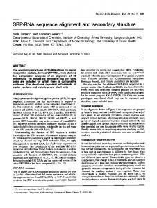
1.1.1 Transfer RNA (tRNA) These are short sequences of close to 76 bases that have been sequenced in many organisms (So$ ll, 1993 ; Sprinzl et al. 1996), and that form a very well-defined clover-leaf secondary structure. The middle three bases of the central loop are the anticodon, which pair with the appropriate codon in the mRNA. The tRNAs are charged with an amino acid at the 3h end, and this is incorporated into a growing peptide chain during protein synthesis. Each organism must have at least one type of tRNA for every amino acid. Figure 1 shows a ‘ ribbon ’ diagram of the L-shaped tertiary structure of tRNA interacting with an aminoacyl tRNA-synthetase protein. The tRNA (usually considered a small RNA) is approximately the same size as a medium sized protein (approximately 350 amino acids long in this case). This picture emphasises the relatively large scale of RNA helices compared to α-helices in proteins, and also the fact that specific interactions between proteins and RNA can occur by fitting together of three dimensional structures in a similar way to molecular recognition and specific interactions between different proteins.
RNA secondary structure
201
Fig. 1. Crystal structure of tRNA(Gln) and glutaminyl–tRNA synthetase (Arnez & Steitz, 1996) prepared from PDB file 1QRS (Berman et al. 2000). The anticodon loop is uppermost and the 3h acceptor end of the tRNA is on the bottom right.
1.1.2 Messenger RNA (mRNA) An mRNA molecule is a copy of one of the strands of a region of DNA, and is typically several thousand bases long. The mRNA has a central portion that codes for a protein and functions as a template during protein synthesis. The 5h and 3h untranslated regions (UTRs) at the two ends are not translated into proteins. Although it is the sequence not the structure of mRNA which is paramount, elements of structure within the UTRs are thought to influence the binding of the ribosome, the rate of expression of the protein, and the lifetime of the mRNA in the cell (Klaff et al. 1996). The recently discovered tmRNA has features of both tRNA and mRNA, and is responsible for adding a C terminal peptide tag to the incomplete protein product of a broken mRNA (Williams, 2000).
1.1.3 Ribosomal RNA (rRNA) Ribosomes are particles of about 250 A/ in diameter that are composed of two sub-units, and that are present in multiple copies in every cell. Each contains three types of rRNA and about 56 different proteins (Moore, 1993 ; Noller, 1993 ; Zimmermann & Dahlberg, 1996). The small sub-unit contains SSU rRNA, often called 16S RNA (approx. 1500 bases). The large sub-unit contains LSU rRNA, or 23S RNA (approx. 2500 bases) and a smaller 5S RNA
202
Paul G. Higgs
(approx. 120 bases). The S numbers refer to the sedimentation coefficients of these molecules in eubacteria. The corresponding molecules are larger in eukaryotes and smaller in mitochondria, so that the same molecules can have different S numbers. Ribosomes are responsible for protein synthesis – they possess binding sites for mRNA and tRNA, and they move sequentially along the mRNA template, acting on one codon at a time. It is thought that the rRNA molecules are responsible at least partly for the catalytic activity of the ribosome. Ribosomal RNAs have been sequenced in very many organisms and large databases are available giving sequence alignments and structural models (Van de Peer et al. 1998 ; De Rijk et al. 1998 ; Maidak et al. 1999 ; Gutell et al. 2000). 1.1.4 Other ribonucleoprotein particles Several other RNAs also occur in association with proteins. Ribonuclease P consists of an RNA of approximately 350 nucleotides bound to a protein of approximately 120 amino acids. This is responsible for cleavage of precursor tRNA molecules to form mature tRNAs (Pace & Brown, 1995 ; Brown, 1999). The Signal Recognition Particle contains an RNA (approx. 300 nucleotides) and several different proteins. It is thought to bind to ribosomes on the membrane of the endoplasmic reticulum, and to influence the translocation of newly synthesised proteins across the ER membrane (Zweib & Samuelsson, 2000). The splicing of introns from mRNAs is performed by small nuclear ribonucleoproteins, which contain short RNA sequences called U RNAs (Baserga & Steitz, 1993 ; Zweib, 1997). 1.1.5 Viruses and viroids RNA viruses are particles consisting of one or more molecules of RNA contained within a protein coat (Gibbs et al. 1995). The RNA is the genome of the virus : it carries out the role normally played by DNA as a store of genetic information. Almost all organisms can act as hosts for RNA viruses. Some of the simplest viruses are bacteriophages, such as Qβ and MS2, that multiply inside bacterial cells. Other examples include plant pathogens like Tobacco Mosaic Virus, and human pathogens like influenza and human immunodeficiency virus (HIV). Structures within the viral RNA are often important for the function of viruses, for example the internal ribosome entry site, or IRES element, in picornaviruses (Jackson & Kaminski, 1995), pseudoknot structures that cause ribosomal frameshifting (Theimer & Giedroc, 1999 ; Giedroc et al. 2000), and various structural elements in MS2 phage (Olsthoorn & van Duin, 1996 ; Groeneveldt et al. 1995). Like viruses, viroids are also parasites that multiply only inside host cells (Pelchat et al. 2000). However, viroids are not enclosed in protein capsids. They are usually plant pathogens consisting of small circular RNAs of about 500 nucleotides, e.g. potato spindle tuber viroid (Repsilber et al. 1999). 1.1.6 Ribozymes RNA molecules having catalytic activity are known as ribozymes (whereas enzymes are catalytic proteins). Ribonuclease P is thus a ribozyme and rRNA can probably be considered as one. The term ribozyme is more usually applied to short structural motifs like the
RNA secondary structure
203
hammerhead and hairpin ribozymes. These occur in plant viroid RNA and cause self cleavage of the strand (Pan et al. 1993). These motifs can be separated out as short strands that cause cleavage of other RNAs. By targeting specific mRNAs or viral RNAs, these ribozymes can be adapted for therapeutic use (James & Gibson, 1998). Whilst most introns are spliced out of their mRNAs by the spliceosome, as described above, the Group I and Group II introns are self-splicing. These introns sequences are able to fold to a particular structure that forms the active site for the splicing reaction (Cech, 1993 ; Sclavi et al. 1998 ; Treiber et al. 1998). The relatively recent discovery of natural RNA catalysts has led to interest in the development of artificial ribozymes by in vitro selection methods (Breaker & Joyce, 1994). The range of catalytic roles that can now be performed by ribozymes is quite wide (Tarasow & Eaton, 1998). This lends support to the ‘ RNA World ’ hypothesis, which argues that there was a time shortly after the origin of life (between approx. 4n2 and 3n8i10* years ago) when both the genetics and the metabolism of organisms were based on RNA (Joyce, 1991 ; Maynard Smith & Szathmary, 1995).
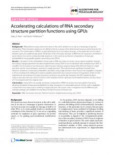
1.2 Elements of RNA secondary structure RNA molecules have the potential to form into helical structures wherever there are two parts of the sequence that are complementary. Hydrogen bonds are possible between C$G and A$U pairs, and also between less stable G$U pairs. Isolated base pairs are usually unstable ; hence, helices usually consist of at least two pairs. There are rarely more than 10 pairs in an unbroken helix. Much of the stability of the helix comes from attractive stacking interactions between successive base pairs, which are in roughly parallel planes. The free energy of the helix is usually assumed to obey a nearest neighbour model – i.e. there is a free energy term for each two successive base pairs. In the example below, we have an AU stacked with a CG, a CG with a CG, and a CG with a GC. 5h–ACCG–3h 3h–UGGC–5h Both energy and entropy changes of helix formation can be measured in experiments with short nucleotide sequences (Freier et al. 1986), using either calorimetry or optical methods. Melting curves generated by these experiments are fitted to the expected results for a twostate transition using a van’t Hoff analysis. SantaLucia & Turner (1997) have reviewed recent progress with these thermodynamic measurements, and have discussed several slightly different models for the stacking free energy in helices. Various types of single-stranded regions occur between helices, known as hairpin loops (connecting the two sides of a single helix), bulges and internal loops (connecting two helices) and multi-branched loops (connecting three or more helices). An example of the structure of a moderately large RNA illustrating all these types of loop is shown in Fig. 2. There are free energy penalties associated with loops due to the loss in entropy of the chain when the loop ends are constrained. Some of the loop free energies have been measured experimentally. In general, loop parameters are known with lower accuracy than helix parameters (SantaLucia & Turner, 1998) and there are some aspects, such as multi-branched loops, about which there are no thermodynamic data. It is usually assumed that the loop free
204
Paul G. Higgs
Fig. 2. The secondary structure of ribonuclease P from E. coli is a typical example of a complex secondary structure of a moderately large sequence (reproduced from Brown, 1999).
energies depend on the number of unpaired bases in the loop but not on the base sequence. Tetraloops are exceptions to this. These are particular sequences of four single stranded bases (e.g. GNRA, where N is any base and R is a purine) that occur frequently in length-four
RNA secondary structure
205
hairpin loops, and that have increased thermodynamic stability due to interactions between the unpaired bases. In structure prediction algorithms we need to assign a free energy to each possible structure, and to compare the relative thermodynamic stabilities of alternative structures of a given sequence. Reasonable estimates are available for thermodynamic parameters that have not been directly measured. The free energy of a complete molecular structure is usually estimated by combining the free energy terms coming from the different parts of a secondary structure. Computational algorithms that do this are discussed in Section 2. 1.3 Secondary structure versus tertiary structure Progress with determination of secondary structure has proceeded more rapidly than for tertiary structure and until recently there has been little experimental information on tertiary structure. This review also focuses mostly on secondary structure, and therefore in this section we discuss what can and what cannot be learned from secondary structure alone. We argue that work at the secondary structure level is still of considerable importance, despite the recent increase in our knowledge of RNA tertiary structure. A secondary structure can be thought of as a list of the base pairs present in the structure. To form a valid secondary structure, base pairs must satisfy several constraints. Let the bases in a sequence be numbered from 1 to N. A base pair may form between positions i and j if the bases are complementary, and if Q jki Q � 4, since there must usually be at least three unpaired bases in a hairpin loop. Let bases k and l form another allowed pair. The pair k–l is said to be compatible with the pair i–j if the two pairs can be present in a structure simultaneously. Pairs are compatible if they are non-overlapping (e.g. i j k l ) or if one is nested within the other (e.g. i k l j ). The third case, where the pairs are interlocking (e.g. i k j l ) is known as a pseudoknot. Such pairs are assumed to be incompatible for most dynamic programming routines, for reasons described below. An allowed secondary structure is a set of base pairs that are all compatible with each other. A secondary structure diagram tells us only about the base pairing pattern and gives us no information about the relative positions of structures in three dimensions. The positioning of the different helices on the page is adjusted for artistic convenience, and is arranged so that the chain does not cross itself. Helices forming pseudoknots can be added to this diagram, as with helices P4 and P6 in ribonuclease P (Fig. 2). When tertiary structure information is also available, the secondary structure diagram can be changed to show, as far as is possible in two dimensions, which parts of the molecule are in close proximity. For example, the secondary structure representation of the self-splicing group I intron (Cech et al. 1994 ; Damberger & Gutell, 1994) demonstrates the folding back of the P5abc domain onto the P4 and P6 helices. This requires a diagram where the chain crosses itself on the page. A similar type of representation for ribonuclease P has also been used by Massire et al. (1998). Most secondary structure diagrams are not drawn with the benefit of hindsight from tertiary structures, and therefore we need to be wary about reading too much into them. Nevertheless the secondary structure of RNA is quite informative. It tells us a considerable amount about the domain structure of the molecule, and allows positions of important sites within the structure to be located. It is much more informative about the shape of the molecule than the secondary structure representation for a protein, which is just a linear string with positions of α helices and β sheets noted.
206
Paul G. Higgs
The most important argument in favour of secondary structure is that RNA helices are thermodynamically strongly bonded. The usual view of RNA folding is that it is hierarchical (Pyle & Green, 1995 ; Brion & Westhof, 1997 ; Tinoco & Bustamente, 1999). It is thought that stable secondary structures form first, and that tertiary structures form afterwards as the molecule is able to bend around the flexible single stranded regions. The strength of the tertiary interactions that arise in the later stages of folding is usually thought to be too small to disrupt previously formed secondary structures. Wu & Tinoco (1998) have given an interesting counter example to this in the 56 nucleotide P5abc domain of the Tetrahymena group I intron. The secondary structure of this domain in solution (as obtained from NMR studies) differs by several moderately large changes from that in the crystal structure of the full P4–P6 domain because of additional tertiary interactions that form in the crystal. Nevertheless it still seems to be the general rule that tertiary interactions can only change the weakest of secondary structural elements, such as moving a few base pairs in a relatively unstable helix. Some estimates for strengths of tertiary interactions are now beginning to become available (Silverman & Cech, 1999) that may help to make this argument more concrete. This picture again contrasts with that in proteins, where individual secondary structure elements (like α helices) are often not stable on their own, and therefore it is much more difficult to separate secondary and tertiary structures from one another. For many years the amount of tertiary structure data for RNA has lagged far behind that for proteins due to the difficulty of crystallizing RNAs. This situation is now changing, and an increasing number of RNA structures are being obtained by NMR and X-ray crystallography (Holbrook & Kim, 1997 ; Kjems & Egebjerg, 1998). Leontis & Westhof (1998) have given a detailed review of various possible non-standard configurations of base pairs in 3D. Images of tertiary structures have also been collected on a website (Su$ hnel, 1997). Discussion of individual structures is outside the scope of this article ; however, it is worth noting some of the tertiary motifs that appear to be important in holding together RNA structure domains (reviewed in full by Hermann & Patel, 1999). Base triples can form when a base in a loop interacts with a pair of bases in a helix in another part of the molecule. Attractive interactions can occur between loops due to stacking of interlocking bases between the loops. Base pairing can occur between hairpin loops (kissing hairpins) in such a way that the pairs in the loops are quasi-continuous with the two hairpin helices. Hydrogen bonding can also occur between unpaired bases and riboses in the backbone elsewhere in the molecule (the ribose zipper motif ). The common feature of all these structures is that they anchor together different structural domains and thus stabilise large-scale tertiary structure. Metal ions have an important influence on RNA structure because they screen out repulsive electrostatic interactions between negatively charged phosphate groups on the RNA backbone. RNA folding is very strongly influenced by magnesium ions in particular, and several cases are known in which Mg#+ ions are bound tightly into specific plates in RNA tertiary structures (Misra & Draper, 1998 ; Hermann & Patel, 1999). Multi-branched loops can play a key role in tertiary structure because they can act as flexible hinges between otherwise fairly rigid helical domains. Stacking of base pairs between the ends of pairs of helices meeting at multi-branched loops can determine the relative positions of these helices, and such stacking can again be influenced by Mg#+ ions. This occurs, for example, in the three-way junction in the hammerhead ribozyme (Lilley, 1998). Pseudoknots have traditionally been excluded from the definition of secondary structure (Section 1.2). One reason for this is that the most common form of dynamic programming
RNA secondary structure
207
structure prediction algorithm cannot account for pseudoknots. From large secondary structures, like the small sub-unit and large sub-unit rRNAs, it appears that most helices conform to the non-overlapping or nested arrangements and that we do not lose much by excluding the interlocking pseudoknot arrangement. However, it is becoming clear that certain types of pseudoknot are common in real RNAs, particularly viral RNAs, and that these often have a functional role. The number of known pseudoknots has reached the point where a specific pseudoknot database has been established (van Batenburg et al. 2000). Tertiary structure information on pseudoknots is also becoming available (Westhof & Jaeger, 1992 ; Hilbers et al. 1998, Hermann & Patel, 1999). More recent dynamic programming algorithms do not have the restriction against pseudoknots (Rivas & Eddy, 1999, see Section 2). Kinetic folding algorithms and genetic algorithms can relatively easily generate pseudoknot configurations, and programs of this type have been available for some time (Abrahams et al. 1990). The practical problem is that there is little thermodynamic information available on pseudoknot stability. Melting behaviour of a few specific pseudoknots has recently been studied in detail, however (Theimer et al. 1998 ; Theimer & Giedroc, 1999). Gultyaev et al. (1999) have also proposed a set of thermodynamic parameters for pseudoknots for use in structure prediction programs. Known tertiary structures are mostly for small motifs involving a small number of helices. Modelling of tertiary structure at a similar scale can be done by molecular dynamics (Auffinger & Westhof, 1998 ; Hermann & Westhof, 1998). This is a useful way to explore the distribution of metal ions around an RNA molecule. However, molecular dynamics is too slow for simulations of the complete molecular folding process, as is well known to also be the case for protein folding. Other tertiary modelling techniques assume that the secondary structure is known, and look for a 3D structure consistent with the 2D constraints (Major, 1998). From their discussion of RNA folding mechanisms, Tinoco & Bustamante (1999) also conclude that the logical way to obtain a tertiary structure prediction is first to predict the secondary structure and then to look for possible elements of tertiary structure that are consistent with it. Thus, there is no substitute for secondary structure prediction for large RNAs of biological interest, and there is still considerable research activity in methods of secondary structure determination (Section 2). We conclude this section with two arguments from a theoretical viewpoint for the importance of RNA secondary structure. The first argument is that the secondary structure model is both realistic and theoretically tractable. The model uses real thermodynamic parameters that, for the most part, have been directly measured in experiment, and it is sufficiently realistic to be able to predict structures for particular biological sequences. At the same time, it is sufficiently simple for analysis with statistical physics methods : the minimum free energy state and the partition function can be calculated exactly. Theoretical questions about the folding mechanism and equilibrium thermodynamics can therefore be addressed (Section 3). In the protein folding field there is a much larger gap between theoretical models (usually on simple lattices with random chains) and realistic modelling of particular proteins. The second argument is that secondary structure has an important influence on the way that RNA sequences evolve. This has implications for those interested in the mechanisms of molecular evolution or the use of RNA sequences in phylogenetic methods. More generally, the sequence to structure mapping of RNAs provides a way of generating fitness landscapes, and thus leads to some important insights into evolutionary processes in general (see Section 4).
208
Paul G. Higgs
2. Theoretical and computational methods for RNA secondary structure determination 2.1 Dynamic programming algorithms The most thermodynamically stable structure of a molecule is the one with the minimum free energy (MFE). An initial aim of structure prediction programs is therefore to determine the MFE structure. There are a finite number of valid secondary structures for any given sequence, according to the criteria of Section 1.3. The MFE structure can, in principle, be obtained by considering every possible base pairing pattern and calculating the free energy for each using the experimentally determined set of energy rules. The number of possible structures increases exponentially with the length of the molecule, N, hence one would expect exhaustive enumeration to be limited to very short sequences. However, the calculation can actually be done in a time of order N$ using what is known as dynamic programming. The method works by writing a recursion relation that breaks down the structure of a large sequence into a sum of smaller parts. The word ‘ dynamic ’ is somewhat unfortunate : it should be remembered that these algorithms deal with equilibrium properties of molecules and have nothing to do with molecular dynamics or with folding kinetics. There are a number of sophisticated implementations of RNA structure programs using dynamic programming that will be discussed below. However, as an illustration of the method we will discuss how the algorithm works with a very simple set of energy rules. In this model, each pair in a helix contributes an energy of k1 unit, and there are no penalties associated with loops. The groundstate structure is just the one with the maximum number of base pairs. For this reason, this model is referred to as the ‘ maximum matching model ’ (Nussinov & Jacobson, 1980). Let εij be the energy of the bond between bases i and j, which is k1 for a complementary pair, and j_ otherwise. We wish to obtain Eij, the minimum energy of the part of the sequence from bases i to j inclusive. Suppose the last base j is bonded to another base k in the sequence. This creates two regions of the chain from i to kk1, and from kj1 to jk1, which cannot interact with each other (because pseudoknots are forbidden). The minimum energy with the jkk bond constraint is therefore Ei,k− jEk+ ,jjεkj. If base j is not paired then the minimum energy is Ei,j− . Hence the " " " minimum energy of all allowed configurations is
0
1
min Eij l min Ei,j− , (E jEk+ ,j− jεkj) . " i � k � jk4 i,k−" " "
(1)
This means that the minimum energy of any chain segment can always be expressed in terms of the minimum energies of smaller segments. We know by definition that Eii l 0 for jki 4, hence we can build up the Eij values for chains of successively longer lengths until the complete chain value E N is obtained. At each stage, it is necessary to store a pointer to which " of the configurations was the minimum energy one. The configuration corresponding to E N " can then be obtained by backtracking through this array of pointers. The structure with the maximum number of pairs is usually quite different from the structure of a real RNA. When we wish to determine the MFE structure of a real biological sequence it is necessary to use the full set of energy parameters described in Section 1.2. Dynamic programming methods have been developed over a number of years (Nussinov & Jacobson, 1980 ; Waterman & Smith, 1986 ; Zuker, 1989 ; Durbin et al. 1998) and have been implemented in a number of freely available software packages such as mfold (Zuker, 1998)
RNA secondary structure
209
and the Vienna RNA package (Hofacker et al. 1994). The recursion relations used in these programs are considerably more complicated because they have to account for penalties of formation of loops of different types and there are many special cases to be considered. Nevertheless the algorithms remain efficient, and still scale as N$ for the full energy parameters. An important theoretical development was to calculate the partition function (McCaskill, 1990) rather than just the MFE structure. Here we give the result only for the simple maximum matching case, because we use this model again further in Section 3.4. The partition function Zij for the section of chain from bases i to j inclusive can be obtained using the following recursion, beginning with Zii l Zi,i− l 1 for all i : " j−% Zij l Zi,j− j � Zi,k− Zk+ ,j− exp(kεkj\kT ). " " " "
(2)
k=i
From this one can calculate the probability pij that bases i and j are paired in the complete equilibrium ensemble of structures : Z Z exp(kεij\kT ) pij l ",i−" j+",N . ZN "
(3)
If i and j are not complementary, pij l 0, because the exponential factor gives zero when εij is j_. The values of the pij give information about alternative structures to the MFE structure. It may be that for a given base i there are several j for which the pairing probability is quite large, indicating that there are several alternative structures for this part of the model with similar free energies. In contrast, other possible pairs in the molecule may have pij virtually equal to 1, indicating that all the possible structures with significant equilibrium probability contain this pair. The dot-plot representation implemented in the Vienna package (Hofacker et al. 1994) gives a graphical representation of these pairing probabilities, and allows variable and non-variable regions of the structure to be identified. It should be remembered that for the full set of energy parameters the E values are free energies (they contain both entropy and energy terms), whereas in the simplified model above they are just energies. The minimum free energy structure for real sequences therefore changes with temperature. At room temperatures most sequences fold to a structure with several helices. As the temperature is raised the structure melts – the completely unfolded state has the lowest free energy at high temperature. The weightings of the different structures in the partition function algorithm also depend on temperature. From the partition function algorithm it is possible to calculate the heat capacity and the mean fraction of the molecule that is in a helical state as a function of temperature – i.e. it is possible to predict the ‘ melting curve ’ for an individual sequence. Again this is implemented in the Vienna package. In the standard model for the energy parameters, the entropy of loops is treated as an empirical parameter that is measured from data for small loops and then extrapolated to larger loops in an approximate way. Recent progress has been made in theoretical estimation of loop entropies by treating unpaired sections of chain using a lattice polymer model (Chen & Dill, 1998). The partition function can again be calculated with this model, and predictions can be made for the shape of the melting curve. Chen & Dill (2000) claim these predictions are considerably better than predictions using the Vienna package. Tøstesen (1999) also finds surprising sensitivity of the shape of the melting curve to sequence details such as the
210
Paul G. Higgs
positioning of GC and AU base pairs within a long helix. Detailed experimental measurements of the melting curves for real RNA sequences have been made in a few cases (Privalov & Filimonov, 1978 ; Laing & Draper, 1994 ; Theimer & Giedroc, 1999). Further measurements of this type would clearly be useful to refine and test these theoretical models. Another quantity of interest, closely related to the partition function, is the density of states, i.e. the distribution of the number of structures as a function of energy. Higgs (1993) gave a calculation of the density of states for secondary structures that was based on a ‘ bruteforce ’ enumeration method rather than dynamic programming. This was used effectively on tRNAs, to look at the size of the energy gap between the MFE structure and alternative structures, and to show that tRNAs have considerably greater thermodynamic stability than random sequences of comparable length. Recently a dynamic programming algorithm for the density of states has been written (Wuchty et al. 1999) that has also been used for tRNA study. Although it is in principle more efficient than the brute-force method, the complexity is such that it is unlikely to be practical for molecules much longer than tRNAs. The model of Chen & Dill (2000) also calculates densities of states. In this case, they are configurational states of the lattice polymer model, not just secondary structure states. A recent extension of the dynamic programming technique (Rivas & Eddy, 1999) allows for pseudoknots, with the exception of only the most complex of pseudoknot topologies. This is an important theoretical advance. The algorithm also allows for coaxial stacking between helices at junctions, which had been argued to be important experimentally, but which had not been implemented in the dynamic programming stage of folding algorithms (Walter et al. 1994). The algorithm is of increased complexity – O(N') in time instead of O(N$) – and has so far only been shown to be practical for short sequences. It should be emphasised, however, that the usual dynamic programming routine excluding pseudoknots is rather rapid, and the method can be used for very long sequences, such as complete viral genomes, in realistic times. Developments in the algorithms that increase efficiency are still being made (Lyngsø et al. 1999). Essentially, speed and size are no longer issues, and the key point is now the reliability of the predictions (see Section 3.1).
2.2 Kinetic folding algorithms Dynamic programming methods work on the assumption that real RNAs will be found in their minimum free energy structure – i.e. they assume the molecule is in equilibrium. However, the stacking energies of RNA helices can be large compared to the thermal energy kT, and so it can be difficult to dissociate them once formed. There is therefore the possibility that the kinetics of folding of the molecule is important in determining the final structure, and that the structures which we find for real molecules may be those that form most easily, rather than those that are lowest in free energy. Experimental evidence on folding kinetics is discussed in Section 3.2. Here we concentrate on computational methods that are based on folding kinetics. The simplest kinetic algorithms consist of the sequential addition of helices to structures in such a way that the free energy is lowered at each step. The algorithm stops when no further helix can be added that will lower the free energy. Abrahams et al. (1990) implemented a folding routine that sequentially adds helices that are compatible with the existing structure at each step. The next helix added is the one that lowers the free energy by the largest amount.
RNA secondary structure
211
A recent variant on this (Li & Wu, 1998) is to add helices sequentially in a random order, provided the free energy is lowered. The procedure is repeated many times and the structure predicted is composed of the helices that appear most frequently in the set of structures generated. As explained above, kinetic based routines can generate pseudoknots relatively easily. The sequential routine of Abrahams et al. (1990) does this, and includes a full model for the energy of pseudoknot configurations. Several authors have used Monte Carlo simulations to simulate the folding process of RNA molecules (Fernandez, 1992 ; Mironov & Lebedev, 1993 ; Schmitz & Steger, 1996 ; Fernandez et al. 1999). These algorithms go further than sequential addition programs because they allow both making and breaking of helices, and there is a time scale associated with the simulation that can be related to real time. To explain the method, we describe our own implementation of ‘ Pair Kinetics ’ and ‘ Helix Kinetics ’ folding algorithms (Higgs & Morgan, 1995 ; Morgan, 1998). Some results from these programs are given in Section 3.3. In the Pair Kinetics program, a rate of formation is assigned to each possible base pair that is compatible with the existing secondary structure, and a rate of removal (i.e. helix unzipping) for every base pair that is already present. One reaction is then selected with a probability proportional to its rate. Thus, fast reactions are more likely to happen than slow ones, although any allowed reaction can occur with non-zero probability. The configuration is then updated to reflect this step of addition or removal of a base pair. The time represented by this single Monte Carlo step is the reciprocal of the sum of the rates of all the possible reactions. Rates are assigned using the Metropolis algorithm : a move that increases the free energy by an amount ∆G has a rate r exp(k∆G\kT ), and a move that lowers the free energy " has a rate r . Here, r is a rate constant that is chosen so that the timescale of the simulation " " is as close as possible to experimental measurements of RNA folding timescales. The free energy changes are calculated using the same energy model as used for dynamic programming algorithms. Choosing the rates in this way ensures that the kinetic system is consistent with equilibrium thermodynamics. Flamm et al. (2000) have recently implemented a kinetic folding routine that works by addition and removal of single base pairs, and introduces other smallscale moves that speed up the reorganisation of secondary structures, such as the migration of a bulge loop along a stem. Pair Kinetics programs can be slow on large sequences since elementary moves are very small changes. We also use a Helix Kinetics program in which an elementary move is the addition or removal of a whole helix rather than just a single base pair (Higgs & Morgan, 1995 ; Morgan, 1998). This cuts out configurations with partially formed helices, but it allows more rapid simulation of longer molecules. the Metropolis algorithm is not appropriate for assigning rates in this case. Formation of a hairpin, for example, involves the loss of entropy of the loop before the gain of the stacking energy of the helix. We may consider the partially formed helix as an intermediate that gives an activation energy for the helix-formation process. This is an important factor in determining the formation rate of a helix. In contrast, the ratio of helix formation and break-up rates depends on the free energy difference between the two end configurations, and not on the activation energy. RNA molecules are synthesised sequentially from their 5h ends by polymerase enzymes that use another complementary strand (either RNA or DNA) as a template. Folding may occur on a comparable timescale to synthesis, so that structure at the 5h end may form before the 3h end of the molecule is complete. Most of the kinetic routines allow the addition of bases to the sequence during the folding process.
212
Paul G. Higgs
Another kinetic approach is to estimate reaction rates in the same way as for Monte Carlo methods, and then to numerically solve the set of differential equations for the probabilities of finding the molecule in each configuration (Tacker et al. 1994 ; Breton et al. 1997). A problem with this method is that one can only include a small number of the exponential number of possible configurations and it is therefore necessary to pre-select the configurations that are thought to be important. This has been done in one example by Gultyaev et al. (1995), who compare their genetic algorithm results with the kinetic equations method. To end this section on kinetic methods, we note that Evers & Giegerich (1999) have produced the ‘ RNA movies ’ software package for visualising sets of RNA secondary structures, such as those generated by kinetic folding routines. An animated sequence of images is produced such that one structure gradually changes into another. This has been used to study RNA sequences that are known to switch reversibly between configurations (Giegerich et al. 1999).
2.3 Genetic algorithms Genetic algorithms (GAs) are a well-known technique for solving complex optimisation problems by imitating biological evolution (Mitchell, 1996). A population of trial solutions to the problem is stored, each of which has a fitness that is a measure of how well the solution solves the required problem. The solutions are treated as individuals that replicate, mutate and possibly recombine. Evolution gradually leads to the creation and selection of high fitness solutions. GAs can be applied to a very large range of problems, and are usually used when there is no exact method of finding the optimum. For RNA folding, however, dynamic programming routines do give an exact optimum (within the limits of the thermodynamic model), and therefore there would be little point in using a GA to find the MFE structure. The use of GAs for RNA has more in common with kinetic folding routines than equilibrium ones. Several methods have been proposed, e.g. van Batenburg et al. (1995), Benedetti & Morosetti (1995), Shapiro & Wu (1996). These work by storing a population of alternative structures for a given sequence. Fitness is a function of the free energy of the structures : low free energy structures have higher fitness and reproduce more frequently. These structures may mutate, by addition or removal of a helix, or may recombine, by producing a hybrid structure containing helices from two different parent structures. The series of structures that forms during a GA simulation can be used to predict the folding pathway. The number of generations of mutation and selection in the GA is qualitatively equivalent to time ; however, there is no quantitative measure of time as there is with Monte Carlo. The selection stage in the GA incorporates thermodynamics in a qualitative way, but there is no guarantee that the population will converge to any meaningful equilibrium state. GAs have a great deal of flexibility in the way that mutation and crossover are implemented and the way the fitness of any given structure is determined. This may be considered a disadvantage, because there is no theoretical basis on which to decide these details other than by trial and error, and because mutation and crossover have no direct relationship to the physical behaviour of the molecule. It may also be considered an advantage, because tuning the method carefully allows realistic results to be obtained. In practice GAs have proved a useful tool in analysis of RNA folding pathways when combined
RNA secondary structure
213
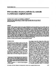
with biological insight into the molecules under investigation (Gultyaev et al. 1995, 1998a, 1998b ; Franch et al. 1997 ; Currey & Shapiro, 1997 ; Wu & Shapiro, 1999). 2.4 Comparative methods When sequences are available for a given molecule from a number of different species it is possible to obtain a very good idea of the secondary structure by comparative sequence analysis (Woese & Pace, 1993 ; Gutell et al. 1992, 1994 ; Gutell, 1996). The assumption is that molecules with the same function in different species will have the same structure, and therefore it is necessary to find a structure that is an allowable base-pairing pattern for all the sequences. The method begins by doing a multiple alignment of all sequences. If one has a reasonably diverse set of sequences then there will be variation in the base that occurs at any one position in the alignment. The method searches for sites that covary – i.e. where changes in one site are correlated with changes in another site. If the sites vary in such a way as to maintain base pairing ability, this is strong evidence that a base pair is present at this position. For example, several of the sequences may have A and U at two sites, whilst the rest may have G and C in these positions. Changes like this are known as compensatory mutations, since mutation occurring on one side of a helix will often disrupt the structure, but this can be compensated for by a second mutation on the other side. This occurs frequently in RNA evolution. an example of an alignment for tRNA(Ala) is shown in Fig. 3. There have been compensatory changes in nearly all the helical parts of this molecule. For the comparative method to work there must be a reasonable amount of variation between the sequences so that compensatory mutations can be identified, but not too much variation, otherwise it will not be possible to make a reliable sequence alignment. The method works best where there are many sequences available. The currently accepted structures of most large RNAs, such as small and large sub-unit rRNAs, have been deduced by this method. It is generally accepted that structures obtained this way are more reliable than those obtained using thermodynamic methods, and should be considered as the ‘ true ’ structure. Disadvantages of the comparative method are that it cannot work on a single sequence, and that it cannot say anything about alternative structures of a sequence, or about folding pathways or thermodynamic stability. Although the method does give a good predicted structure in many cases, it does not tell us why or how the molecule folds to the appropriate structure. The presence of a conserved structural motif is often an indication of a functional role for that section of RNA. Hence there is a practical interest in locating sequence regions that fold to particular structural motifs. Several algorithms have been proposed that search for structural patterns in RNA sequence data (Chevalet & Michot, 1992 ; Laferrie' re et al. 1994). When there is a large amount of information on a structural motif, it is easy to spot that motif with a high level of confidence. A prime example of this is the tRNAscan program of Lowe & Eddy (1997) that searches genomic DNA sequences to find the sites of tRNA genes, using the known structure of the tRNA molecule and known conserved features of the sequences. For a family of RNAs with a conserved sequence, a statistical model of the structure can be built up (Eddy & Durbin, 1994 ; Durbin et al. 1998). Other sequences can then be checked against the model to see whether regions of these sequences conform to the conserved structure of the family. The comparatively derived structures in sequence databases, such as those for rRNA, have
214 Paul G. Higgs Fig. 3. An alignment of tRNA(Ala) sequences for widely differing species, showing conserved secondary structure and compensatory mutations. The cloverleaf secondary structure is indicated by bracket notation. Positions where there have been compensatory changes on both sides of the helix and denoted . In the columns denoted X, there has been a change from a GC to a GU pair, also maintaining pairing ability.
RNA secondary structure
215
gradually been built up manually over long periods of time, and have been refined as further sequences were added to the alignments. For new sets of sequences without known structure, there is considerable interest in methods that can automatically locate conserved structures using comparative methods, or combinations of comparative and thermodynamical methods. Hofacker et al. (1998) have analysed virus genomes using an algorithm of this type. Families of related sequences are first aligned using a standard method of multiple sequence alignment. Individual MFE structures are then predicted for each sequence. A consensus structure is obtained by choosing pairs of columns from the alignment for which the corresponding bases are paired in the MFE structure of as many as possible of the sequences in the set. For regions with conflicting information from the different sequences, no consensus structure is predicted. This reflects the likely situation in real families of virus sequences, where only certain regions of the sequences are likely to have conserved structures, whilst other regions may differ widely. The method of Lu$ ck et al. (1996) also begins with a thermodynamic structure prediction for each sequence, and a sequence alignment. Their algorithm calculates the probabilities pk(i j ) that bases i and j are paired in each sequence k. This is done by using either the partition function folding algorithm, or by counting the frequency of occurrence of the pair in a set of suboptimal structures. A weighted combination of these probabilities is then used to generate a probability pc(i j ) of pairing of i and j in the consensus structure. Both these methods have been shown to give useful results for relatively small sets of sequences, where there would be insufficient evidence from purely comparative methods. The Maximum Weighted Matching method (Tabaska et al. 1998) also begins with a set of prealigned sequences. A score is assigned that reflects the likelihood of any given column of the sequence alignment pairing with any other column. The set of paired columns that have the highest total score is found using a graph theory algorithm very much like the dynamic programming methods. Base triples and pseudoknots can also be found with this method. The above methods all begin with multiple sequence alignments and attempt to deduce structures consistent with the alignment. Structural information is, however, not used in generating the alignment in the first place. Konings & Hogeweg (1989) have discussed ways of aligning structures rather than sequences. A structure can be represented by a string of symbols, and multiple alignment methods can then be used to align these strings in the usual way. This type of algorithm can align an unpaired base with an unpaired base, the left side of a pair with another left side, or a right side with a right side ; however, it does not take the full structural information into account. At the point in the algorithm when the left side of a pair is reached, it is not yet known where the corresponding right side will be. Ideally, one would wish to have a positive score in the alignment algorithm only if both sides of a pair were simultaneously aligned with each other. Gorodkin et al. (1987a, b) have developed a structural alignment algorithm that does exactly this. The method uses a dynamic programming method that takes a time O(N%) for two sequences of length N, whereas straightforward alignment of strings takes a time O(N#). This method has been shown to be practical for locating short conserved motifs in families of sequences where there is no prior structural information, such as sequences derived from SELEX in vitro selection experiments. The method does not take account of the thermodynamics of folding, it merely counts a positive score when two sites that can form a Watson–Crick or GU pair in one sequence are aligned with two sites that can form a pair in another sequence. An important simplification is made by disallowing multi-branched loops. If these are included, the algorithm becomes O(N'), which is impractical for most applications. We note that Sankoff (1985) already
216
Paul G. Higgs
proposed an algorithm capable of simultaneously aligning and finding the structure of S sequences, using thermodynamic energy parameters and allowing for branched structures. Whilst this is a technical tour-de-force, it has proved impractical since the time required is O(N$S). If exact structure-based alignment is difficult, another approach is to use simulated annealing programs to gradually reshuffle alignments to give better scoring configurations (Kim et al. 1996). This method is stochastic, and therefore is not guaranteed to converge to an optimal configuration, but the advantage is that more complex scoring systems can be used. The method of Bouthinon & Soldano (1999) is another variant on the theme of searching for conserved secondary structures. It uses a representation of the topological pattern of helices, and combines thermodynamic and comparative information. The reason for the presence of conserved structures is, of course, that the sequences are evolutionarily related. Whilst there are many structure prediction programs and many programs dealing with molecular evolution and phylogenetics, there are few that combine these two. The quality of the trees obtained in phylogenetic methods depends crucially on the quality of the sequence alignment used, and structural information helps to obtain a good alignment. It therefore makes sense to use evolutionary information in sequence alignment and structure prediction. Goldman et al. (1996) developed a method for simultaneous secondary structure prediction and molecular phylogenetics of proteins. Knudsen & Hein (1999) have used a similar idea for RNA. The method calculates the likelihood of a data set of aligned sequences, given a model of sequence evolution for paired and unpaired regions, and given a secondary structure. From this the consensus secondary structure with the maximum a posteriori probability can be obtained. Models of sequence evolution for RNA are discussed in more detail in Section 4. One method of structure prediction that does not fit well under any of the subheadings of this section is the SAPSSARN program (Gaspin & Westhof, 1995). This finds sets of suboptimal secondary structures that are consistent with a set of user-specified constraints. These constraints may incorporate experimental information. This program has been combined with the interactive ESSA package (Chetouani et al. 1997), which also contains routines for drawing of complex secondary structures, and programs for alignment and comparative analysis. Where structural information is available from experiment, this can be combined with comparative sequence analysis and 3D molecular modelling to give a predicted model of both tertiary and secondary structure. Excellent examples of this are the 3D model structures of ribonuclease P RNA (Westhof & Altman, 1994 ; Chen et al. 1998 ; Massire et al. 1998). There are now large numbers of RNA folding software packages available. Links to many of these are on the ‘ RNA world ’ web site (Su$ hnel, 1997). Space prevents mentioning all of them. This review has attempted to emphasise methods and algorithms rather than software implementations and user interfaces.
3. RNA thermodynamics and folding mechanisms 3.1 The reliability of minimum free energy structure prediction There have been several studies that assess the accuracy of minimum free energy structure predictions by comparing the results with comparatively derived structures (which are taken
RNA secondary structure
217
to be the true biological ones). Generally, thermodynamic methods work well for short sequences. In a survey of the complete tRNA database (Higgs, 1995) it was found that 85 % of clover leaf helices were correctly predicted. For longer sequences, results are poorer. Zuker & Jacobson (1995) found a mean of 49 % correctly predicted helices in a sample of 15 SSU rRNAs. Konings & Gutell (1995) considered a large sample of SSU rRNAs and found between 10 % and 81 % correctly predicted base pairs, with a mean of 46 %. Results on LSU rRNA were very similar (Fields & Gutell, 1996). Morgan & Higgs (1996) studied a selection of long RNAs including SSU and LSU rRNAs and RNase P, and found a mean of 55 %. One possible reason for these relatively low scores is that the energy rules used in the model may not be sufficiently accurate to distinguish the correct structure as being the MFE one. This is quite possible if there are several alternatives with similar energy values. Le et al. (1993) have deliberately exploited the uncertainty in the free energy parameters in a method of structure prediction. They use many alternative sets of energy parameters that fluctuate about the estimated value and calculate a structure for each set. The final predicted structure is obtained from a consensus of these results. The mfold program can output a set of alternative structures within a specified free energy range above the minimum, and it might be expected that the correct structure would be among these alternatives, even if it is not the absolute minimum with the parameter set used. Konings & Gutell (1995) found that the best of these suboptimal structures was only 4–9 % better than the MFE structure, however. Certain refinements have been made recently to the energy model, such as tetra-loops and stacking of the ends of helices within multi-branched loops, and these have led to slight improvements of the results. It is likely that more such special cases will be found in future. The comparative structures for the rRNAs contain some non-canonical base pairs, like GA pairs, which are not permitted in the secondary structure model (they will usually be treated like internal loops). Fields & Gutell (1996) found that the accuracy of prediction decreased substantially with the fraction of non-canonical pairs. This suggests that additional energy rules are needed to account for these properly. It should also be remembered that the present energy rules do not include tertiary interactions or interactions with proteins (such as the ribosomal proteins in the case of rRNA). These interactions will certainly lower the free energy, but this will only make a substantial difference to the predicted structure if some structures are systematically lowered more than others. We have no way of knowing how much difference this would make. Whatever the underlying reason for the relatively low accuracy of MFE methods, it is clear that there is room for improvement as regards practical methods of structure prediction. One line of attack is to try to distinguish regions predicted with high certainty from less certain regions. Zuker & Jacobson (1995, 1998) define a helix to be ‘ well-determined ’ if it occurs frequently within the set of sub-optimal structures. They have shown that well-determined helices are more accurately predicted than average. A mean of 81 % of the welldetermined helices are present in the comparative structure. This is important as a way of avoiding false positive predictions of helix positions, although the well-determined helices represent a relatively small fraction of the total helices. Another similar idea is to use the base pair probabilities which can be calculated from the partition function algorithm. If pij is the pairing probability of bases i and j, then the Shannon entropy of base i can be defined as Si lkΣj pij ln pij. Huynen et al. (1997) have shown that bases with lower Si are more accurately predicted. Low Si occurs when a base is almost always in the same configuration in all low energy configurations. Since there are few alternatives for this base it is
218
Paul G. Higgs
Fig. 4. Equilibrium unfolding pathway of a pseudoknot. Reproduced from Theimer & Giedroc (1999).
likely that its configuration will be correctly predicted. A simpler definition of welldeterminedness obtainable from the pair probabilities is simply to take the maximum pij for each i. If this is close to 1, the base is well-determined (Huynen et al. 1996b ; Rauscher et al. 1997). The reliability of structure prediction methods is gradually improving, but it is likely that the comparative method will always be the preferred method for cases where there are many homologous sequences available. There is a lot of potential in combining these methods in cases where there are several sequences available but no clear structure has yet been established from comparative analysis alone. This has been done with several types of viral RNA recently (Lu$ ck et al. 1996 ; Rauscher et al. 1997). 3.2 The relevance of RNA folding kinetics Interest in RNA folding kinetics has built up rapidly over the past few years, mostly due to a large number of detailed studies on the folding of the Tetrahymena group I intron (Sclavi et al. 1998 ; Treiber et al. 1998 ; Nikolcheva & Woodson, 1999 ; Fang et al. 1999 ; Pan et al. 2000 ; Chaulk & MacMillan, 2000). Reviews of this field have been given by Treiber & Williamson (1999) and Batey & Doudna (1998). On the basis of this work it is clear that the energy landscape for large RNAs is a rugged one, and that molecules can get trapped in metastable states from which it is difficult to escape. This means that there is a wide range of timescales relevant to the folding process. Whilst some individual helices can form in milliseconds, formation of larger secondary structural domains (possibly involving reorganisation of certain helices) can take seconds, and formation of the final active tertiary structure for the whole molecule can take minutes. It is worth distinguishing between equilibrium folding pathways and truly kinetic pathways. Folding\unfolding can be induced by gradual change of temperature (e.g. Laing & Draper, 1994), or by gradual change of concentrations of Mg#+ or urea (e.g. Shelton et al. 1999). This leads to an equilibrium pathway of intermediate states between fully folded and fully unfolded structures. Each intermediate structure should be the lowest free energy structure at the intermediate conditions, and the pathway should be reversible. An interesting example of this is the temperature controlled unfolding pathway of a pseudoknot that promotes ribosomal frameshifting in a retrovirus (Theimer & Giedroc, 1999). This is reproduced in Fig. 4. The full pseudoknot contains an unpaired base, A , between the two "&
RNA secondary structure
219
helices, and a bulge, A , in one helix. The lower helix melts first because of the destabilising $& effect of the bulge. After the lower helix has melted the upper helix can extend by pairing of A with a previously inaccessible U base. The upper helix then melts as the temperature is "& further raised. In contrast to this, a truly kinetic pathway is not reversible, and intermediates do not necessarily correspond to low free energy states. This is the case in most of the studies of group I intron folding listed above, where folding is initiated by a sudden change in solution conditions. Fang et al. (1999) have also studied folding rates of ribonuclease P RNA initiated by changing Mg#+ concentration. Another type of kinetic folding pathway is that occurring when RNA folds during synthesis. In this case the relative rates of synthesis and helix folding and unfolding are important to determine the folding pathway taken. One example is the detailed experimental study of the sequential folding of potato spindle tuber viroid RNA during transcription (Repsilber et al. 1999). Other examples are given in Section 3.3. below. One question arising from this is whether natural folding pathways end in the MFE state. The fact that structures predicted by MFE algorithms only partially agree with known biological ones can be put down to limitations in the thermodynamic parameters used, as in the previous section. However, rather than assume that the model is insufficient and that the molecules are really in their MFE state, we could instead conclude that the model is essentially correct and that the molecules are not in their MFE state due to kinetic effects. We have investigated this possibility by analysing the MFE structures of large RNAs (Morgan & Higgs, 1996). We studied the way the accuracy of prediction depends on the sequence length, by finding the MFE structure of domains of varying sizes taken from within large molecules. A domain was defined as a region of the sequence enclosed by the two ends of a helix. It was found that � 90 % correctly predicted pairs were obtained for domains shorter than 50 nucleotides. The accuracy decreased to around 80 % for domain sizes around 100, and for sizes larger than about 200, the accuracy fluctuated around about 55 %. This latter figure was the average value of the percentage of correct pairs in the MFE structures of the complete molecules. We also observed that the free energies of domains of length 100 occurring in the comparative structure were substantially below the mean value for the MFE of domains of comparable size, whereas the reverse was true for larger domains. This can be interpreted in terms of folding kinetics (Morgan & Higgs, 1996) in the following way. The term ‘ hierarchical folding ’ of RNA is sometimes used to describe the fact that secondary structure is likely to form before tertiary structure (Brion & Westhof, 1997 ; Tinoco & Bustamante, 1999). We also expect there to be a hierarchy between different secondary structural elements. Short-range helices, such as individual hairpin loops, should form rapidly, since the two halves of the helix are in close proximity. Longer-range helices will form more slowly, and may only form when previous folding of short-range helices in between brings together the two distant halves of the long-range helix. We therefore expect that progressively larger secondary structure domains should form during the folding process. Larger domains should form by rearranging and combining some of the smaller elements. This ‘ coarsening ’ of the domain structure is driven by free energy minimisation. However, rearrangement of secondary structure involves crossing potentially large energy barriers between structures, because some helices have to be broken up before other more stable ones can be added, as shown in Fig. 5. As the size of domains increases the size of the barriers increases (see Section 3.3), and therefore the time taken for structural reorganisation also increases. There will come a point where the energy barriers will become too large to
220
Paul G. Higgs
Fig. 5. Schematic representation of the reorganisation of secondary structure during RNA folding leading to the formation of progressively larger domains.
be overcome by thermal fluctuations on a biologically reasonable timescale. The result will be a structure containing a combination of domains of a moderate size that are frozen in their local MFE states, rather than a global MFE structure. If there are any very long-range helices in the final structure, these would presumably form at a late stage, and they would have to fit in between the pre-formed medium sized domains. The general argument for coarsening of domain structures applies to configurational relaxation of many physical systems (e.g. domain sizes in magnetic systems, or formation of crystallites after quenching). Thus we argue that energy barriers to structural rearrangement are bound to disrupt the folding process and prevent formation of the MFE state for sufficiently large molecules. How relevant this theoretical argument is for real RNAs depends on whether the freezing in of structure happens on a length scale smaller than the total length of a real RNA, and on a time scale comparable with folding times of real molecules. The observations of Morgan & Higgs (1996) are exactly what would be expected according to this hierarchical picture of secondary structure reorganisation : domains smaller than about 100 nucleotides seem to be in their MFE structure, whilst the large scale structure appears to be an assembly of these medium sized domains. It is of course difficult to separate out the possible effects of freezing in of structure during folding from the effects of inaccuracies in the energy parameters used in the MFE program, and we expect that both these factors are important. Nevertheless, the length scale of 100 that emerged from our study makes sense for a number of reasons. Firstly, over 75 % of helices in the comparative structures have ranges of under 100. This is true for both LSU and SSU rRNAs even though LSU is much longer (Fields & Gutell, 1996). Thus real molecules find it easier to form smaller domains. The dynamic programming methods predict a larger proportion of long range helices than actually occur. We also know that well-defined tertiary structures can begin to form for sequences of about this size (e.g. tRNA, length 76). Once tertiary interactions form, this provides another stabilising factor on these medium-sized domains that will slow down subsequent structural rearrangement and promote the freezing in of existing structures. Many
RNA secondary structure
221
large RNAs form part of ribonucleoprotein particles in which there is close association with specific proteins (e.g. the ribosomal RNAs, and other examples in Section 1.1). Once the shape of medium-sized domains is established, this will facilitate the binding of proteins, and protein binding will again act to stabilise the RNA domains and prevent any further rearrangement. It is intriguing that moderate size RNA domains are of similar size to typical globular proteins – we can imagine the assembly or ribosomes as the fitting together of building blocks composed of proteins and RNA domains. There has been considerable progress with the determination of the 3D structures of ribosomes recently (Frank, 1997 ; Ban et al. 1999 ; Clemons et al. 1999), and the relative positioning of many of the proteins and the rRNAs is known in some detail. It is also known that Tetrahymena IVS folds considerably faster in vivo than in vitro. This suggests a role for RNA binding proteins that stabilise domains of native structure (Brion & Westhof, 1997 ; Weeks, 1997). The presence of chaperone proteins to assist in RNA folding has also been suggested (Thirumalai & Woodson, 1996). An interesting point regarding long-range and short-range helices has been made by Galzitskaya & Finkelstein (1996) and Galzitskaya (1997). They have argued that the stacking energy in the helices of natural RNAs increases with the range of the helix. Long-range helices are apparently more stable than short-range ones because there are a larger number of GC pairs in long-range helices. The argument is that short-range helices can form relatively easily, whereas longer-range ones form with difficulty because of the kinetic problems associated with bringing the ends into proximity. Therefore, if the required functional structure uses long-range helices, evolution selects a sequence with unusually stable stacking energy for these helices. In simulations of random chains, it was shown that ‘ geometrically edited ’ sequences, in which long-range interactions are adjusted to be larger on average than short range ones, tend to fold more rapidly than chains with randomly assigned interaction strengths. The implication is that, by this mechanism, evolution is able to select sequences with more reliable folding kinetics (see also Section 4.2). 3.3 Examples of RNA folding kinetics simulations Having argued rather generally above for the importance of folding kinetics, in this section we discuss several examples of particular sequences where folding kinetics has been studied in simulations, and where kinetics is important for understanding the structure and\or function of the molecule. Qβ replicase is an RNA-dependent RNA polymerase that is responsible for replicating the Qβ bacteriophage genome within the bacterial host cell. The ‘ plus strand ’ genome is used as a template to synthesise the complementary ‘ minus strand ’, which is then used as a template to produce another copy of the plus strand. The system has been used in in vitro experiments on RNA evolution for many years (Pace & Spiegelman, 1966 ; Biebricher et al. 1983). In addition to template-dependent replication, it has been found that, in certain experimental conditions, Qβ replicase can synthesise RNA from individual nucleotides without an initial template (Biebricher et al. 1986). The chain lengths of early replicating template-free products are between 30 and 45 nucleotides. It is found that their primary sequences are not related, but the secondary structures of replicating sequences show significant similarities, consisting of a single 5h hairpin structure and an unstructured 3h terminus. The sequences are optimised so that both the plus and minus strands fold to the
222 Paul G. Higgs
Fig. 6. The metastable active structure and the stable groundstate structure for the plus and the minus strands of the SV-11 (Biebricher & Luce, 1992).
RNA secondary structure
223
same structure. This is unusual and demonstrates the effect of selection : since the 5h end of one strand is complementary to the 3h end of the other, we might expect the two strands to have mirror image structures. The fact that the two strands have the same structure is made possible by the inclusion of GU pairs in the stems at strategic places. We also note that, because of GU pairs, the mirror image argument tends not to apply to most RNAs : for typical sequences, the structures of the two complementary strands would be rather dissimilar. The early products of template-free replication are not replicated particularly efficiently, and they undergo further evolution to create optimised sequences with chain lengths in the range 80–250 bases (Munishkin et al. 1988, 1991 ; Biebricher & Luce 1992, 1993). Under certain experimental conditions a sequence of length 115 nucleotides called SV-11 is consistently selected. This is a recombinant sequence that is almost a palindrome. The groundstate structure for both the plus and minus strands of SV-11 is almost a perfect hairpin (see Fig. 6). However, it has been shown that the groundstate structure is unable to replicate. The active template is a metastable structure formed during replication (Biebricher & Luce, 1992). The metastable states of both strands contain a 5h hairpin structure and an unstructured 3h terminus. SV-11 is special in the sense that both the plus and the complementary minus strand are able to fold to essentially the same structure, and this aids replication efficiency. We estimate that the difference in free energy between the structures of the stable and metastable states is approximately 27 kcal\mol for the plus strand. Since the thermal energy kT is approximately 0n6 kcal\mol, this difference is around 45 kT. In an equilibrium situation the fraction of molecules in the metastable state would therefore be negligible. The fact that SV11 is efficiently replicated means that it must remain for long periods of time in the metastable state, and that there must be large energy barriers preventing rearrangement to the groundstate. We simulated the folding of SV-11 using the Monte-Carlo Pair Kinetics algorithm described in Section 2.2. (Morgan, 1998). Simulations were performed in which folding was allowed during the growth and in which folding occurred from a completely synthesised chain with no secondary structure. 100 runs were carried out for each strand for each set of starting conditions. Curves A B and C in Fig. 7 show three runs in which folding of the minus strand occurs during synthesis. The growth rate of the molecule was taken to be 50 nucleotides per second, although this rate could be varied considerably without changing the outcome. The metastable state was formed repeatably in this case. When folding was initiated after complete synthesis of the sequence (curves D and E), a variety of structures similar to the groundstate was found that have free energies significantly lower than the metastable state. In simulations where the metastable state was formed, it was never observed to convert to the groundstate, even on the longest of our simulation runs, which was several orders of magnitude longer than the time period shown in Fig. 7. This is consistent with the experimental observation (Biebricher & Luce, 1992) that SV-11 remains in the metastable state for at least a period of a few hours at room temperature before eventually converting to the groundstate, whereas it does so much more quickly after short boiling. These results with the Pair Kinetics program give essentially the same conclusions as those of Higgs & Morgan (1995), which were obtained with an early version of the Helix Kinetics program. Flamm et al. (2000) have also simulated folding of SV-11 with a Pair Kinetics program. They observe that the metastable state can also form when folding from the complete molecule. This difference with our results probably reflects differences in the rates assigned to different elementary reaction steps between the programs. More testing of these programs
224
Paul G. Higgs
–10·0
Energy (kcal/mol)
–30·0
–50·0
C
A
–Em
B
–70·0
D E
–90·0 0·0
5·0
10·0
15·0
–Es
Time (s)
Fig. 7. Free energy of secondary structures formed during the folding of the SV-11 minus strand. In runs A$C, folding occurs during synthesis. In runs D and E, folding occurs after synthesis. The drop in free energy from 0 to around k70 kcal\mol occurs too rapidly to be seen on this scale.
will be required in order to refine the way the rates are calculated. We also note that, as one stand is used as a template, its structure is disrupted by the replicase. Therefore, the template strand will refold sequentially each time it is copied, as the replicase moves from one end to the other. The refolding pathway of the template may therefore be very similar to the folding pathway when the molecule is first synthesised. RNA folding kinetics has also been implicated in control of the expression of the maturation protein of the MS2 phage. MS2 is another plus strand RNA virus similar to Qβ, having a length of approximately 3500 bases and coding for four proteins that are required for replication of the RNA genome and for assembly of the virus particle. One copy of the maturation protein is required in every virus particle. The coding region of this gene begins 130 nucleotides from the 5h end of the genome. The MFE structure of the 5h end is shown in Fig. 8. The Shine–Dalgarno region (SD) is the binding site for ribosomes during translation of the maturation protein. In the MFE structure this region is bound to an upstream complementary sequence (UCS) in a stable eight-base pair helix. When this helix is formed, ribosome binding is blocked, and protein synthesis cannot occur. The level of expression of the maturation protein is controlled by the kinetics of folding of the RNA (Groeneveld et al. 1995). Ribosome binding, and hence gene expression, is only possible in a short window of time between synthesis of the SD region itself and the formation of the helix between the SD and the UCS. The alternative hypothesis is that the structure is in equilibrium and that ribosome binding occurs when the helix is dissociated by thermal fluctuations. This can be rejected, as explained below. We have simulated the folding of the 5h of the wild type MS2 phage and also of several mutant sequences studied by Groeneveldt et al. (1995). In the U32C mutant, the UG pair in
RNA secondary structure
225
Fig. 8. Secondary structure of the 5h end of MS2 phage RNA, redrawn from Groeneveldt et al. (1995).
the middle of the helix is replaced by a CG pair, hence the helix is stabilised by approximate 3 kcal\mol. This would decrease the equilibrium probability of the helix being dissociated by two orders of magnitude, however no effect was observed on the gene expression rate. In the SA mutant the clover leaf structure between the UCS and SD regions is replaced by a short hairpin loop. Since the stacking of the main helix is unaffected by this, there should be little change in gene expression according to the equilibrium hypothesis. However, a tenfold decrease in expression rate is actually observed. In the CC3435AA mutant two CG pairs in the helix and disrupted to form AG mismatches. This severely destabilises the helix and should lead to an increase of expression by several orders of magnitude according to the equilibrium hypothesis. In fact, only a fivefold increase is observed. Results of our Monte Carlo simulations are shown in Fig. 9. Each curve shows the probability that the SD region is exposed (average over MC runs) as a function of time since initiation of sequence synthesis. Each curve is zero until the SD is synthesised, goes through a maximum whilst the SD region is free, and returns to a very low level after the helix with the UCS is formed. We would expect the level of gene expression to be proportional to the
226
Paul G. Higgs
CC3435AA
Average prob. SD free
0·2
0·1 WT & U32C
SA 0·0 0·0
2·0
4·0 Time (s)
6·0
8·0
Fig. 9. The accessibility of the SD sequence as a function of time during the folding of wild-type MS2 phage RNA and three mutant sequences.
area under the curve. In fact the results correlate quite well with the experimental observations – the WT and U32C are almost indistinguishable, the SA cure has about one tenth the area, and the CC3435AA curve has about twice the area. Our simulations therefore confirm the argument for the importance of folding kinetics in this system, and the areas are at least qualitatively in agreement with the changes in the levels of expression measured. Direct experimental measures of the folding rate have also been performed (Poot et al. 1997). In these experiments, the molecule is denatured at 70 mC and the kinetics of renaturation at 30 mC is then studied. The molecule apparently takes several minutes to refold, whereas the time scale in the simulations (Fig. 9) for folding during synthesis is seconds. It is easy to be out by a large factor in the time scale in simulations, because energy factors that determine reaction rates appear in exponential terms (i.e. Boltzmann factors). A calibration has to be made of all the rates relative to the rate of the smallest change (zipping up of a base pair). Additional experimental data on the time scale of small structural rearrangements in real RNAs would help to make these programs more quantitative. In the case of MS2 there is also the interesting possibility that refolding after renaturation is considerably slower than folding during synthesis, although we have not tested this with simulations. There have been several genetic algorithm studies of folding kinetics. The case of potato spindle tuber viroid RNA (Gultyaev et al. 1998a) is similar to the SV-11 case discussed above, in that metastable structures arise during the sequential folding of the RNA that are important for viroid replication. These structures are also evolutionarily conserved. Another wellstudied example of RNA folding kinetics is related to the regulation replication of the ColE1 plasmid, a circular DNA sequence present in multiple copies in E. coli bacteria. An RNA
RNA secondary structure
227
sequence known as RNA II, encoded by the plasmid, binds to one of the DNA strands and acts as a primer for DNA replication. The primer activity can be inhibited by another plasmid-encoded RNA (RNA I) which binds in an antisense fashion to RNA II (Polisky, 1988). Point mutations in the RNA II sequence increase the copy number of plasmids in the cell because they affect the folding kinetics of RNA II. It has been shown that the copy number mutations do not affect the stable minimum free energy structure of RNA II, nor do they disrupt the complementary binding of RNA I and RNA II. However, they increase the stability of a metastable structure that is formed during the folding of RNA II. The metastable structure is eventually transformed to the MFE structure, but its presence influences the binding of RNA I and RNA II. Hence the lifetime of the metastable structure is important in controlling the overall replication rate of the plasmid. The kinetics of folding of RNA II has been studied in detail using a genetic algorithm (Gultyaev et al. 1995), and we have also obtained similar results by Monte Carlo simulations (Morgan, 1998). Although metastable states have been seen in several examples above, we might think that transfer RNA would be a case where straightforward folding to the groundstate might be expected. We know that the MFE algorithm correctly predicts the clover leaf structure in most cases. The fact that tRNA can be crystallised and X-ray structures can be obtained also suggests that the structure is relatively stable and inflexible. Despite this there are cases where even tRNA can get into a wrongly folded state (Kearns, 1974 ; Uhlenbeck, 1995) if it is denatured and the conditions of refolding are not carefully controlled. Flamm et al. (2000) have simulated the folding of tRNA(Phe) using a Pair Kinetics program. Using the algorithm for enumeration of low free energy secondary structures (Wuchty et al. 1999) they showed that there were six principal low free energy structures, each with a corresponding group of small variants. Figure 10 shows a tree of the 50 lowest local minima, arranged so that the heights of the branch points represent the energy barriers between structures. 50 % of the folding trajectories ended up in the clover leaf basin of attraction in this case. This is a larger percentage than any of the other structures, even though the cloverleaf structure is not the global minimum structure according to the energy rules used. We would expect that the outcome of these simulations would be very sensitive to energy rules. Small changes in energy parameters might make the clover leaf structure slightly lower in free energy than some of the other basins of attraction, particularly if stacking between helices in the four-way junction were included and tertiary interactions between the loops were added. Such changes would influence the kinetics. Also the kinetics will be strongly dependent on rates of individual reaction steps included in the program, and these are not known with any certainty. Therefore, we probably cannot conclude from Fig. 10 that only 50 % of real tRNAs form the right structure (it would be surprising if nature were not more efficient than this), but we can conclude that metastable states and large energy barriers are present even in molecules as simple as tRNA. 3.4 RNA as a disordered system The previous section was written from a biological point of view, and aimed to describe the structures of naturally occurring sequences as realistically as possible. This section will take a statistical physics viewpoint, and will consider generic properties of random sequences. A ‘ disordered system ’ in physics is one in which the structure or the interactions are disrupted in a random way. For example, a ferromagnet is a regular array of atoms in which the
228 Paul G. Higgs
Fig. 10. Tree representation of the 50 lowest local minima structures in tRNA(Phe), reproduced from Flamm et al. (2000). Percentages on the right give the probabilities of folding pathways leading to the six principal basins of attractions.
RNA secondary structure
229
magnetic moment (spins) of neighbouring atoms interact so that they want to be parallel to each other. A disordered system can be formed changing the interactions so that some pairs of neighbours want to be parallel (ferromagnetic interaction) and some want to be antiparallel (anti-ferromagnetic interaction). This is known as a spin glass. Spin glasses have unusual equilibrium properties and phase transitions, including non-self-averaging behaviour and replica symmetry breaking (Me! zard et al. 1987), which have generated a great deal of interest among statistical physicists. A key concept in disordered systems is frustration : a frustrated system is one in which not all favourable energetic interactions can be satisfied simultaneously. In the spin glass example, it is not possible to find any configuration of the spins for which every pair of neighbours with a ferromagnetic interaction has parallel spins and every pair of neighbours with an anti-ferromagnetic interaction has anti-parallel spins. The lowest energy configurations in such systems are compromises that try to satisfy as many as possible favourable interactions at one time. There may be many alternative compromises that can be reached, hence we expect a rugged energy landscape with many alternative low energy minima. The term ‘ glass ’ is applied to spin glasses because of the slow dynamics of magnetic relaxation that is caused by the presence of the rugged energy landscape. A second example of a disordered system is the random heteropolymer. Whereas a homopolymer is one in which all the monomers are equivalent, a heteropolymer is composed of different types of monomers, some of which attract each other and some of which repel. One type of heteropolymer used for protein models is composed of a random sequence of hydrophobic and polar monomers on a lattice (e.g. Dill et al. 1995). Can RNA really be considered as a random heteropolymer or a disordered system ? The number of different complementary pairs that could form in a random RNA sequence of bases of length N is of order N#, whereas the number of pairs which can be present at the same time in any one structure is of order N. This means that the sequence is frustrated, in the disordered system sense, because it is not possible to form all the attractive intramolecular bonds at the same time. We expect that sequences may have alternative structures that are very different from one another and yet have very similar energies. We also expect that there may be large energy barriers between alternative low energy structures, because it is necessary to break one set of base pairs apart before it is possible to start adding another set. In other words, we expect that RNA folding is a problem with a rugged energy landscape, and we would like to say as much as possible about this landscape. We will use the maximum matching model described in Section 2.1. Since all states have integer energy in this model, it turns out that there are many exactly degenerate states. We have shown (Higgs, 1996 ; Morgan & Higgs, 1998) that the minimum energy varies linearly with sequence length (E- "k0n368 N ), and that the total number of states Ω and the number of degenerate groundstates ω increase exponentially with N, so that lnΩ " 0n533 N, and lnω " 0n068 N. The bars indicate averages over random sequences of equal base frequencies. A typical chain of length 200 has approximately 5i10' degenerate groundstates and there are approximately 70 base pairs in each groundstate. These quantities can all be calculated for any given sequence using recursion relations like those in Section 2.1. Since we have access to the partition function, we can also obtain equilibrium quantities, such as mean energies and specific heat capacities, exactly as a function of temperature, even for large systems (up to N l 1200 was studied by Higgs, 1996). In other disordered system models one is limited to small sizes since there are no algorithms for calculating the partition function. For example, in random heteropolymer models, exact enumeration of all 27-mer configurations on a cubic
230
Paul G. Higgs
lattice can be done, but one cannot go much beyond this. In order to study equilibrium properties of disordered systems, it is usually necessary to do Monte Carlo simulations, using a technique like simulated annealing to ensure that the simulation is not trapped in local minima. Such simulations are difficult precisely because of the rugged landscape nature of the problem that one is trying to study. With the RNA problem equilibrium properties can be found without simulations. One of the principal quantities of interest in disordered systems is the overlap distribution. An overlap is a measure of similarity of two configurations, whilst ‘ distance ’ is a measure of how different they are. Two almost identical configurations have an overlap close to 1 (or a very small distance), whilst two very different configurations have a small overlap and a large distance. In the case of mean field spin glass models, a theoretical treatment of overlaps has been developed using the replica method (Me! zard et al. 1987 ; Binder & Young, 1986). At high temperatures the system can be in a very large number of different configurations. For large systems, all of these configurations tend to be roughly equidistant from one another. The overlap distribution is a narrow peak centred on its mean value – i.e. it is ‘ selfaveraging ’. At low temperatures, the overlap distribution is sensitive to the valleys of low energy configurations in the energy landscape. Some of these are close and some are far apart, hence the overlap distribution is broad, even for large systems. Also the mean overlap fluctuations between samples (i.e. different choices of the random couplings between the spins in the spin glass, or different random RNA sequences), and is said to be ‘ non-self-averaging ’. We have shown (Higgs, 1996) that the maximum matching model of RNA also appears to have a broad non-self-averaging distribution of overlaps at low temperature. The numerical investigation relies on the fact that we can generate a set of randomly chosen configurations with probabilities proportional to their Boltzmann factors – i.e. we can generate an equilibrium ensemble of configurations every easily. The overlaps between all pairs of structures in the set can then be measured. Another interesting property of low energy configurations in spin glass models is that they can be arranged in a hierarchical set of clusters – small valleys within larger valleys within larger valleys. This is known as ‘ ultrametricity ’ (Rammal et al. 1986 ; Me! zard et al. 1987 ; Parisi & Ricci Tersenghi, 2000). For any three structures, three distances can be measured between the three possible pairs. The set of structures is ultrametric if, for any three structures chosen, the two largest distances are equal. Again, our study showed that the distances between the groundstates in the maximum matching model were approximately ultrametric. Two further studies of low temperature properties of random RNAs have appeared recently using a similar model to that of Higgs (1996). Pagnani et al. (2000) consider a chain with two types of monomer a and B, such that A$B bonds are twice as strong as A$A or B$B bonds. The topological rules for pair formation are as in RNA secondary structure. They argue that there is a low-temperature phase with a broad overlap distribution. However, other numerical work with essentially the same model (Hartmann, 1999) concludes that the overlap distribution narrows to zero for long sequences. There are some details of the definition of these models whose significance has yet to be tested. For example, is there any significant difference between sequence with a four-letter ACGU alphabet and a two-letter AB alphabet ? Does the introduction of paired states between identical monomers A$A and B$B affect the outcome – only non-identical monomers may pair in real RNA ? Does the constraint of allowing a minimum number of three unpaired bases in a hairpin loop affect the entropy enough to change the qualitative behaviour ? Despite these unresolved issues, it is
RNA secondary structure
231
clear that there are several similarities between the maximum matching model and mean-field spin glasses, although as yet no formal link has been made between the two models, and we have no analytical theory for the RNA case. Bundschuh & Hwa (1999) have considered a model with a particular stable native structure, and have shown that there is a transition from a low temperature phase, where the molecule is in the native state, to a higher temperature phase, where the molecule adopts a range of possible non-native secondary structures. In the example chosen, the native state is a single hairpin (i.e. the second half of the molecule is complementary to the first). The transition arises in this model because the energy gap between the native state and other possible structures increases in proportion to N, and the entropy lost by confining the molecule to a single state is also proportional to N. The energy term will win for low enough temperature, meaning that there is a well-defined transition in the thermodynamic limit. There is a close parallel between the dynamic programming algorithms for RNA folding and those used for sequence alignment, and the alignment problem in turn is similar to the problem of directed polymers in a random medium (Hwa & La$ ssig, 1996 ; Xiong & Waterman, 1997). If two correlated sequences are aligned (e.g. two genes that diverged from a common ancestor), then there should be a best alignment that has a significantly higher score than the alternatives. This is the equivalent of the native state in the RNA model. If two random sequences are aligned, then the best alignment will have a similar score to the alternatives. This is equivalent to the folding of a random RNA with no well-defined native structure. The relevance of this type of transition to natural RNAs is questionable, however. Real RNAs vary in length over quite a wide range (at least 10#–10%, see Section 1), whereas the length of helices does not change much. Helix length certainly does not increase in proportion to the length of the molecule, as for the hairpin example. If the energy gap between the native state and alternatives does not scale with N, there will not be a well-defined transition. This point was raised previously by Higgs (1993), who compared the melting transition of hairpin molecules with real tRNA sequences and with completely random sequences. Random sequences have a broad melting curve centred at a relatively low temperature, whereas hairpin molecules have a sharper transition at a higher temperature. Natural tRNAs are intermediate between these. The approach to the thermodynamic limit cannot really be studied in natural sequences, because if we compare different types of RNA with different lengths, then the nature of the selective forces acting on the molecules will be different. It is usually assumed that, if structures are far apart in distance, they will be separated by a high energy barrier. We have tested this with RNA (Morgan & Higgs, 1998), using an algorithm for finding barrier heights between alternative groundstates. There are many pathways between two groundstate structures, and the rate at which the molecule proceeds along these pathways will be determined by the highest energy point on the route. The most relevant kinetic pathway at low temperatures will be the one for which this highest point is lowest. In what follows, the ‘ barrier height ’ between two groundstates refers to the height of the highest point on the lowest energy route. The problem of finding the lowest energy route is a complex one, and is similar in nature to the travelling salesman problem. We believe that our algorithm (described by Morgan & Higgs, 1998) produces a good estimate of the lowest barrier for most pairs of structures, but it is not guaranteed to give the optimal solution in every case. Once the barriers have been estimated for every pair of structures in the set of
232
Paul G. Higgs
Fig. 11. Matrix representation of the barriers between each structure in the set for a sequence of length 450. The lighter the shade of grey, the higher the barrier between two structures. the structures are arranged in order so that the hierarchy of clusters can be clearly seen (from Morgan & Higgs, 1998).
groundstates, we can cluster the structures hierarchically according to their barrier heights. It follows from the definition of lowest energy routes that this clustering is exactly ultrametric. The clustering can be represented by a grey scale matrix. An example for one typical random sequence is shown in Fig. 11. The hierarchical structure of the states is clearly visible. The distances between structures are correlated with the barrier heights, but not exactly. Therefore clustering based on distances is only approximately ultrametric. The matrix of distances therefore appears like the matrix of barrier heights with noise added (Fig. 12). We have also shown that the mean barrier height scales with the sequence length approximately as N"/#. This confirms that barrier heights increase with sequence length, which was an important part of our argument about the formation of domains during RNA folding kinetics in Section 3.2 (see Fig. 5). Giegerich et al. (1999) have also considered clustering of alternative structures based on structural similarity and on energy barrier height in order to study sequences that switch between alternative configurations.
RNA secondary structure
233
Fig. 12. Matrix representation of the distances between the same set of structures as Fig. 11. Darker shades indicate greater similarity of structures. The ordering of the structures is the same as in Fig. 11 (from Morgan & Higgs, 1998).
We conclude that the RNA model provides an excellent example of a disordered system for study since we can get much further with the description of the energy landscape than we can with most other models and numerical calculation of equilibrium properties can be done exactly. Theoretical studies of this nature are also important because they shed light on the folding mechanisms of real RNAs.
4. Aspects of RNA evolution 4.1 The relevance of RNA for studies of molecular evolution RNA sequences play an important role in several key areas of molecular evolution studies. This section introduces some of these questions briefly, before proceeding to discuss the influence of RNA secondary structure on sequence evolution in Sections 4.2–4.4.
234
Paul G. Higgs
4.1.1 Molecular phylogenetics Molecular sequences have become widely used for constructing phylogenetic trees (Swofford et al. 1996 ; Li, 1997 ; Page & Holmes, 1998). Many types of computer programs for constructing phylogenetic trees are available. The Phylip website (Felsenstein, 1995) contains references to most of these. Small sub-unit rRNA has proved to be one of the most useful sequences for phylogenetic purposes (Hillis & Dixon, 1991 ; Olsen & Woese, 1993). It has been sequenced in a great variety of species and large comparative databases have been set up (Van de Peer et al. 1998 ; Maidak et al. 1999). The molecule is sufficiently long to contain a large amount of evolutionary information, in comparison to tRNAs and 5S rRNA, which are rather too short to give reliable trees. Since the secondary structure is well conserved it is possible to make reliable alignments of sequences from very diverse groups. The molecule is ubiquitous – it occurs in prokaryotes and eukaryotes, and also in the genomes of mitochondria and chloroplasts. A major discovery made initially by study of SSU rRNA was that there are three fundamental domains of life (Woese et al. 1990) known now as Archaea (or Archaebacteria), Bacteria (or Eubacteria) and Eukarya (or Eukaryotes). As well as these very large-scale trees, the following examples illustrate the way SSU rRNA has yielded phylogenetic information over a range of progressively decreasing scales : $ $ $ $
$
the earliest branching groups of lower eukaryotes (Van de Peer et al. 1996) the relationship between amphibians, birds and mammals (Hedges et al. 1990) the principal groups of mammals (Novacek, 1992) the relationship of toothed whales, baleen whales and sperm whales (Milinkovitch et al. 1993) species within the dog family (Ledje & Arnason, 1996).
The latter examples use mitochondrial SSU rRNA sequences, since these evolve more rapidly than nuclear sequences and are therefore more informative about closely related species. 4.1.2 tRNAs and the genetic code Transfer RNA must be a very old molecule since it is essential to the way that the genetic code is decoded, and all organisms use virtually the same genetic code. The fact that organisms share the same code, and the same protein synthesis machinery is a strong argument that all of current life on earth can be traced back to some single common ancestor. Eigen et al. (1989b) carried out a statistical analysis of the divergence of tRNA sequences in order to obtain an estimate of the age of the genetic code. Their estimate of around 3n8i10* years is close to the estimated time for the demise of the RNA world (Joyce, 1991), and around the time of the earliest conclusive evidence of life in the fossil record (Deamer & Fleischaker, 1994). This emphasises the degree of structure conservation that is found – for almost as long as there has been life on earth, there have been cloverleaf tRNAs functioning in more or less the same way. There have been some speculations on the original role tRNAs might have had in an RNA world before protein synthesis (Maynard Smith & Szathmary, 1995). It is known that tRNAs from mitochondria are much more variable than those in the eukaryotic nucleus and in bacterial genomes. There are several alternative pairing patterns with slightly longer or shorter helices than the standard clover-leaf (Steinberg & Cedergren,
RNA secondary structure
235
1995), and there are exceptional cases where a whole hairpin loop can be missing from the structure. This suggests either a relaxation in the stabilising selection on the structure or an increase in the mutation rate in mitochondria. Lynch (1996) has discussed nuclear and mitochondrial tRNAs in the context of Muller’s ratchet. This is a stochastic process by which unfavourable mutations may accumulate in asexually reproducing organisms despite the action of selection against them (Haigh, 1978 ; Lynch et al. 1993 ; Higgs & Woodcock, 1995 ; Woodcock & Higgs, 1996). Mitochondria are subject to Muller’s ratchet since they are usually inherited from a single parent. 4.1.3 Viruses and quasispecies The Qβ replicase system (discussed in Section 3.3) was one of the first examples of molecular evolution to be studied in vitro. It was apparent from these experiments that the replicase was relatively prone to errors. In fact the error rate was estimated as u l 5i10−% per base. This means that for the viral genome of length N l 4500, the probability of replication without error is only (1ku)N l 0n1. The population of sequences therefore contains many slightly different variants. The quasispecies theory was originally developed to explain these observations. It has been discussed in detail by Eigen et al. (1989a) and Swetina & Schuster (1982). In the simplest version of the theory there is a single high fitness sequence (or master sequence) surrounded in sequence space by many lower fitness variants. Although the master sequence replicates faster than the rest, not all of the offspring copies are identical to the master sequence. Hence there is a competition between mutation (i.e. replication error) and selection. If the error rate is not too large then a balance is reached in which the master sequence is maintained at a finite fraction of the population. If the error rate is larger than a critical value, known as the error threshold, the master sequence disappears from the population. For longer sequences, the error threshold occurs at smaller error rates – i.e. a long sequence requires either a more accurate replication process or a greater selective advantage than a short sequence in order to survive in evolution. There are now many viruses whose sequence evolution has been studied (Gibbs et al. 1995 ; Domingo et al. 1998a, 1998b), and it is thought that many of these operate close to their error thresholds. Replication of RNA viruses is roughly a million times less accurate than DNA replication in eukaryotes. This is one reason why virus genomes are of limited size. However, the variability of sequences in a viral population allows rapid exploration of sequence space and may lead to the discovery of new fitter variants at some distance away from the initial master sequence. Variability also probably helps viruses avoid the immune system. 4.1.4 Fitness landscapes The MFE folding algorithm for RNA can be considered as a mapping from genotype (sequence) to phenotype (structure). There have been detailed studies of the way properties of the MFE structure change as one moves through sequence space (Schuster et al. 1994 ; Gru$ ner et al. 1996). One key observation is that, starting from any point in sequence space, it is possible to find a sequence which folds to any common secondary structure within a small region centred on that point, i.e. it is not necessary to change the sequence very much in order to change the structure considerably. Sequences that fold to each of the common structures are distributed throughout the sequence space in the form of a neutral network. Populations
236
Paul G. Higgs
can evolve along these neutral networks by random drift without changing their structure (Forst et al. 1995 ; Huynen et al. 1996a ; Reidys et al. 1997 ; Stadler, 1999). This is exactly what appears to have happened with real RNA sequences such as tRNA, where the sequences are extremely divergent despite almost exact structure conservation. The neutral network picture is a way of thinking of the effects of compensatory mutations from a sequence space viewpoint. The idea of neutral networks may also turn out to be important for other types of evolution in addition to RNA, and several evolutionary models incorporating a degree of neutrality are now being studied (Gavrilets, 1997 ; Bastolla et al. 1999 ; Bornberg-Bauer & Chan, 1999 ; Taylor & Higgs, 2000). A recent advance in this area is to look at evolutionary transitions between alternative structures. Fontana & Schuster (1998) have simulated evolving populations of RNAs under selection for an optimal structure. The fitness of the population increases in a series of steps as the structure gradually changes towards the optimal one. Neutral sequence evolution is possible between each of these structural changes. 4.2 The interaction between thermodynamics and sequence evolution Since natural selection acts on biological molecules we would expect to see evidence of evolution when we look at RNA sequences and structures. One question that arises naturally is to ask in what way real RNA sequences differ from random ones. We have shown that tRNAs are unusually stable thermodynamically compared with random RNA sequences of the same length and the same base composition (Higgs, 1993, 1995). The groundstate free energy is very low, and there are relatively few alternative structures within a small energy range above the groundstate. The secondary structure tends to melt at a higher temperature than for random sequences. This shows that evolution has had some success in designing molecules with unusual thermodynamic behaviour. A stable structure is presumably essential to the function of the molecule. Some of the modified bases in tRNA are unable to form base pairs. Modified bases therefore act to increase the thermodynamic stability of the groundstate structure, because they prevent the formation of alternative structures that would otherwise compete with the clover leaf. This is shown in theoretical studies of secondary structure (Higgs, 1993 ; Wuchty et al. 1999). Experimental studies of tertiary structure formation also show that there is a difference between native and unmodified tRNAs (Maglott et al. 1998). The native sequence can fold in the absence of Mg#+, whereas the unmodified sequence only forms a stable tertiary structure in the presence of Mg#+. Does a difference between real and random sequences exist for other longer RNAs ? Seffens & Digby (1999) have shown that mRNA sequences also seem to have a lower free energy than expected, and therefore argue that stable secondary structures are selected in coding sequences. This may occur by selection between synonymous codons in such a way that structures can form in the mRNA. The result depends on how the random sequences are created, however. Workman & Krogh (1999) found that if MRNA sequences were shuffled in a way that preserved the frequency of dinucleotide pairs, the original sequences did not have a significantly lower free energy than the shuffled ones. This shows that the dinucleotide frequencies are not simply the product of the two individual base frequencies. Whilst this is evidence for selection of some sort, it does not definitely suggest selection for formation of secondary structure. Another study on large structural RNAs, including rRNA, rRNase P and group I and II introns, shows a greater stability of natural structures than structures of
RNA secondary structure
237
Table 1. Base pair frequencies in seven sets of RNA sequences with conserved secondary structure and a range of overall GjC content tRNA tRNA tRNA general mitoch. archaea RNase-P rRNA-0 rRNA-1 rRNA-2 GjC content Whole sequence Helical regions Base pair frequencies GC CG AU UA GU UG MM Number of sequences Number of pairs
0n532 0n681
0n339 0n448
0n636 0n829
0n594 0n730
0n545 0n656
0n545 0n674
0n535 0n662
0n372 0n260 0n128 0n142 0n043 0n025 0n030 754
0n266 0n121 0n257 0n233 0n046 0n030 0n046 884
0n473 0n320 0n057 0n077 0n031 0n020 0n022 64
0n385 0n296 0n117 0n104 0n050 0n022 0n026 84
0n313 0n265 0n109 0n156 0n075 0n068 0n014 455
0n352 0n298 0n122 0n173 0n020 0n021 0n014 455
0n350 0n292 0n117 0n201 0n015 0n017 0n008 645
21
21
21
80
338
296
304
randomly permuted sequences (Schultes et al. 1999). Non-random patterns in base frequencies in RNA have also been observed by Schultes et al. (1997). They have developed methods of visualising the base composition graphically. Similarities are observed between evolutionarily unrelated sequences, which suggests consistent selective pressures (such as thermodynamic constraints) acting on different types of molecule. Selection for sequences with stable MFE structures is not necessarily an advantage in all cases ; for example, the molecule may require to alternate between configurations. Also, it may be that reproducibility of the folding pathway is more important than low free energy of the groundstate, as suggested by Galzitskaya & Finkelstein (1996). Nevertheless, the fact that secondary structure is strongly conserved in many important RNAs shows that selection is acting to maintain this structure, and we therefore expect that naturally occurring sequences will be biased towards thermodynamic stability. Clear evidence for this is that the frequency of the different types of base pair is greatest for pairs with the greatest thermodynamic stability, as discussed for rRNA by Gutell (1996). Our analysis of base pair frequencies is given in Table 1, which includes several sets of RNA sequences obtained from databases that included a well-established secondary structure model. In each case, the sequence alignment and structure given in the database was taken to be correct. these sequence sets will be described in detail since they are also used in Section 4.4. Transfer RNA gene sequences were taken from the tRNA sequence database (Sprinzl et al. 1996). These were divided into three sets : sequences from mitochondria, sequences from archaea, and a ‘ general ’ set that includes all tRNAs not from mitochondria or archaea. These sets were chosen because mitochondrial sequences have a very low GjC content and archaeal sequences have a very high GjC content, and it is known that this gives significant differences in their thermodynamic properties (Higgs, 1995). Where two or more sequences were found to be identical in the helical regions of the sequence only one of these was included in the set of sequences analysed. The ribonuclease P data set consists of 84
238
Paul G. Higgs
eubacterial RNase P RNAs obtained from the database of Brown (1999). The set denoted rRNA-0, was obtained from the Small Sub-unit Ribosomal RNA database of Van de Peer et al. (1998). One sequence was selected randomly from each genus of eubacteria in order to give a fairly widely diverging set of sequences. The set rRNA-1 consists of the same sequences as rRNA-0, but only a subset of base pairs are included in the analysis (for reasons described in Section 4.4). The final set, rRNA-2, consists of all the sequences from the gamma proteobacteria class of eubacteria, taken from the Small Sub-unit rRNA database. The number of sequences analysed in each set and the number of conserved pairs used in the analysis is shown in the table. The frequencies of the four Watson–Crick pairs plus GU and UG pairs are given in Table 1. There are, in addition, ten types of mismatch combination that occur only rarely in helical regions. These mismatches have all been lumped together into a single MM state for the purposes of the table. The order of the bases in a pair is important : the first mentioned base is the one that is closest to the 5h end of the molecule. Thus it is possible to distinguish unambiguously between a GC and a CG, for example. It can be seen in Table 1 that GC and CG pairs usually have high frequencies (mean 31 %), AU and UA pairs usually have intermediate frequencies (mean 14 %), and GU and UG pairs have low frequencies (mean 3 %). Mismatch states are also rare (mean 2 % MM). These frequencies follow the order of thermodynamic stability of the base pairs. Therefore these results are a clear indication that selection is acting to increase the stability of secondary structures in these molecules. Table 1 also shows the fraction of GjC individual bases in the sequences as a whole. There is a wide variation in content of GjC bases between the different RNA types, indicating that there are different selective effects or mutational biases in different molecules or different groups of organisms. The extremes are the mitochondrial tRNAs (33n9 % GjC) and archaeal tRNAs (63n6 % GjC). However, it is found that the GjC frequency in the helical regions is always higher than the overall GjC frequency in the whole sequence. The frequencies of GjC in the helical regions for the two extreme cases are 44n8 % and 82n9 %. This means that in addition to other mutational and selectional effects that may influence the overall GjC composition in the sequence, there is always selection to increase the GjC content of helices. The frequency of the MM class is comparable with the frequency of GU and UG pairs. This indicates that there is a significant selective disadvantage against mismatches, but this disadvantage is not overwhelming. Mismatches in helical regions can sometimes be tolerated and clearly do not always lead to complete disruption of the molecular structure. Whilst the general patterns in Table 1 are understandable, there is a puzzling feature that the frequency of GC pairs always exceeds of that of CG. The fact that the bias is always in the same direction suggests a consistent selective effect rather than chance ; however, we do not have a convincing explanation for this. The difference appears to be statistically significant. Maximum Likelihood phylogenetic models for RNA helix evolution (Savill et al. 2000) perform significantly better if no symmetry is assumed between GC and CG than if symmetry is imposed. 4.3 Theory of compensatory substitutions in RNA helices As discussed above, compensatory substitutions form the basis of the comparative method of structure determination. Examples of evolutionary studies of compensatory mutations in
RNA secondary structure
239
RNA have been given by Kirby et al. (1995) and Rousset et al. (1991). In this section, we consider the theory of compensatory substitutions (Kimura, 1985 ; Stephan, 1996 ; Higgs, 1998). We will show that, as well as influencing the frequency of base pairs, selection for stable secondary structure also influences the rate of compensatory changes. It is frequently observed that pairs of closely related species differ by a pair of compensatory mutations that have apparently occurred ‘ simultaneously ’. As an example, consider two sites in an RNA-encoding gene that form a base pair in the resulting RNA molecule, and suppose that in one species these sites are G and C bases. In a related species, it is observed that these same sites are A and U. Two substitutions have happened somewhere along the evolutionary pathway separating these two species. Most likely, an initial substitution in the GC sequence has led to formation of a sequence with a GU pair, and a second substitution has occurred sometime later which created the AU sequence. Since mutation rates in most organisms are very low, it is very unlikely that these two events occurred simultaneously in the same individual in the same generation. Thus, from the individual sequence viewpoint, the compensatory change is almost always a two-step process. We refer here to U rather than T bases, although of course all the Us are Ts in the DNA. It should be clear that the mutations are occurring in the DNA genes, whereas selection is acting on the RNA product transcribed from the gene. The RNA sequence will, of course, contain any mutations introduced into the DNA. The substitution process can also be described from the viewpoint of the population. Suppose that a population consists initially of sequences that have a GC pair at a particular point in the molecule, and that a mutation creates an individual that has a GU sequence. This sequence is assumed to be at a slight selective disadvantage due to the reduction in stability of the structure. Many deleterious mutations will be eliminated by selection. However, if the selective disadvantage is not too high, random drift can lead to fixation of GU sequences in the population, or at least to a situation where the majority of the population is GU. If a second mutation occurs in one of these GU sequences to give an AU sequence, this will be at a selective advantage. There is a good chance that the descendants of this AU sequence will increase in frequency until they dominate the population. Once again, the change from GC to AU is a two-step process. However, suppose that the rate of occurrence of the deleterious mutations, u, is considerably less than the selective disadvantage, s, of these mutations. In this case the mutants are kept at a low frequency (of order u\s) by mutation–selection balance. Small numbers of single mutants (GU) nevertheless remain in the population, and one of these can mutate to give the double mutant (AU). The double mutant is now approximately neutral with respect to the majority of the population, which is still GC. Therefore, the double mutant stands a reasonable chance of rising to high frequency by random drift. The mathematics of this process has been studied by Kimura (1985), Stephan (1996) and Higgs (1998) using diffusion equations for gene frequency distributions. For biologically reasonable parameter values, it is expected that at most times the population will be dominated by one or other of the four types of Watson–Crick base pairs, and that occasionally the population will jump between these four alternatives by the compensatory mutation mechanism. Thus, from the population genetics viewpoint, a double substitution in an RNA helix can occur either by a two-step process (with fixation of a deleterious mutation as an intermediate state) or a one-step process (compensatory mutation mechanism). We feel it is important to distinguish between these mechanisms. The key point is that in the one-step mechanism the deleterious mutations remain at very low frequency throughout, and the consensus sequence
240
Paul G. Higgs
of the population changes directly from the initial sequence to the double mutant, whereas in the two-step process the consensus sequence changes twice, and there is a period where the deleterious mutations are at high frequency. In principle, both of these mechanisms can occur in RNA, and what happens in a given situation will depend on mutation rate, population size, and the strength of selection against the intermediate. In the above example, the intermediate was a GU pair. Other double substitutions must occur with mismatches as intermediates, e.g. GC to CG must have a GG or CC intermediate. We would expect this change to occur at a slower rate because the selection against the mismatch is greater than that against a GU pair. In evolutionary models, a transition refers to a change between two purines (A and G) or between two pyrimidines (C and U). A transversion is a change from a purine to a pyrimidine or vice versa. In the RNA case, double transitions between GC and AU or between CG and UA can occur via GU or UG intermediates, and should therefore be relatively rapid. Double transversions, such as those between GC and CG or between GC and UA, must occur via mismatches, and should therefore be slower. If RNA sequences are to be used in molecular phylogenetics, it is important to have a good understanding of what the relative rates of these different substitution processes are. Phylogenetic methods usually assume that each site in the molecule evolves independently of the others. Typically rate-matrix models are used in which each unit on the sequence can be in four different states, representing the four bases. The parameters of the model are the frequencies of the four states and the rates of substitution from one state to another (see examples in Li & Gu (1996), Li (1997)). In RNA helices, the changes in the two sides of a helix are correlated with each other due to the constraint of maintaining the secondary structure. It is therefore preferable to use a model in which the base pair is treated as the fundamental unit, rather than the single base. There have been a variety of previous models of this type : Scho$ niger & von Haeseler (1994) ; Muse (1995) ; Rzhetsky (1995) ; Tillier (1994) ; Tillier & Collins (1995, 1998). Most of these models involve a relatively small number of parameters and make assumptions about the symmetry of the rate matrix. For example, some models assume symmetry between the four Watson–Crick pairs. Nearly all these models allow only single substitutions. Compensatory changes are thus forced to go through a two-step process. Here we wish to make as few as possible assumptions about the nature of the substitution process, since we want to deduce what the mechanism of substitution is from the sequence data. In particular, we wish to allow the possibility of double substitutions. In most phylogenetic studies, there is only a single sequence per species, and there is no information on the minor sequence variations that may exist at very low frequencies. The available sequence should usually be the dominant sequence variant in the population when minor variants are at low frequency. We know from the population genetics theory that the dominant sequence variant can sometimes change by a double substitution. Therefore, this process should be allowed in the rate matrix.
4.4 Rates of compensatory substitutions obtained from sequence analysis In this section, we estimate rates of substitutions of different types in RNA helices in order to test the theoretical predictions above. The sets of sequences analysed are the same as those in Table 1, discussed in Section 4.2. Also as in Table 1, we have lumped all the individual mismatch states into a single state MM. This means that there are seven states used in total.
RNA secondary structure
241
A similar classification of states is used in the model of Tillier & Collins (1998). Here we use the most general reversible seven-state model. By analogy with general reversible four-state models used for single sites (Li & Gu, 1996 ; Waddell & Steel, 1997) we know that the rates of substitution from state i to state j can be written in the form rij l πj αij, where πj is the frequency of state j and the αij form a symmetric matrix (αji l αij). Details of the model are given in Savill et al. (2000), where a full comparison is made between this model and other previously proposed models using statistical methods. Since this model has a large number of free parameters, we might worry that it is over-fitting the data. However, according to likelihood ratio tests, the general reversible model gives a significantly higher likelihood for observed sets of sequence data than other simplified models, and we are justified in using the general model. Here we focus on the physical interpretation of the results obtained with the general model, and refer the reader to Savill et al. (2000) for statistical details. Having defined the rate matrix, we can calculate the probability Pij(t) that a sequence will be in state j at time t given that its ancestor was in state i at time zero. This satisfies the rate equation : dPij l � Pik rkj. dt k
(4)
Only helical regions of the sequences are considered in this analysis. For any two sequences we can count the number of base pairs d which differ. The pairs differ if at least one of the bases in the pair has changed. The fraction of pairs that differ is thus p l d\N, where N is the total number of conserved pairs. We consider each pair of sequences in turn and calculate p. These values are assigned to bins for averaging purposes. We count the number of times Nij( p) that a base pair in state i is aligned with a base pair in state j in sequence pairs of each p value. We then obtain the functions Pij( p), defined by Pij( p) l
Nij( p) . � Nik( p)
(5)
k
For a pair of sequences at separation p, this is the probability of finding a j base pair in one sequence, given that the other sequence has an i at that position. Note that these probability can be obtained directly from the data without use of a theoretical model, and the method does not require knowledge of the phylogenetic tree linking the sequences. The expected value of p is a function of the time t since divergence of the species. The theoretical functions Pij(t) obtained by solving equation (4) are also functions of t. In order to fit the model to the data, the theoretical Pij functions can be plotted as a function of p by treating t as a parameter. This allows direct comparison of the theory and the data points. We use the standard least squares fitting criterion to selection best-fit parameters in the rate matrix – i.e. we minimise the quantity S l Σ(Ptheory kPdata )h, where the sum is over all the data points on all 49 Pij ij ij curves. by fitting over the whole range of p simultaneously we are using all of the data to maximum effect. When finding the optical rate parameters a normalisation condition is always applied to the rate matrix so that the average rate of substitution is 1 per unit time : � πi � rij l 1 � i
j i
This can always be done without changing the fit to the data.
(6)
242
Paul G. Higgs 100·0
80·0
Probability (%)
GC CG
60·0
UA 40·0 UG
AU GU
20·0
0·0 0·0
MM
10·0
20·0
30·0
40·0
50·0
p (%)
Fig. 13. Percentage probabilities Pii( p) that a base pair in state i remains unchanged, shown as a function of the percentage of base pair changes p. Data points are measured in the rRNA-1 set. Curves are the best fit to the seven-state model.
Figure 13 shows the function Pii( p) of the rRNA-1 set. This is the probability that a base pair in the second sequence is in state i given that the first is also in state i. For small p the curves decrease linearly from 100 % with a gradient that we will call the mutability. The figure shows that different pairs change at different rates. GC and CG pairs change slowest (low mutability), and GU, UG and MM pairs change fastest (high mutability). The seven-state model fits the data very well over the whole range of p. The data points lie on rather smooth curves since there are a large number of sequences in the data set. Figure 14 shows the functions Pij( p) for the case where i is CG, and j is each of the other states : this is the probability that the second sequence has changed to state j given that the first is a CG. The most rapidly increasing function is the UA curve, i.e. the most likely change from a CG is that it undergoes a double transition to a UA. The UG curve, which is reached by a single transition, is always lower than the UA curve, indicating that the one-step compensatory mutation mechanism occurs more frequently than fixation of the UG deleterious mutation. The figure also illustrates the difference in rates of double transitions and double transversions. The GC and AU curves are reached by double transversions from CG. These increase less rapidly than the UA (double transition) curve, as was predicted by the argument in Section 4.3. The best-fit rate matrix for the rRNA-1 set is shown in Table 2. The substitution is from the base pair on the left to the base pair listed in the column. The sum of the elements in any row is the mutability of that base pair – i.e. the net rate at which it changes to other states. The * indicates that the diagonal element is equal to minus the mutability of the base pair.
RNA secondary structure
243
16·0
14·0
12·0 UA
Probability (%)
10·0
GC
8·0
6·0 AU 4·0 UG 2·0 GU 0·0 0·0
10·0
20·0
30·0
40·0
50·0
p (%)
Fig. 14. Percentage probabilities Pij( p) of change from the state i l CG to all the other states. Data from the rRNA-1 set.
Table 2. The best-fit rate matrix for the rRNA-1 set
1 2 3 4 5 6 7
AU GU GC UA UG CG MM
1 AU * 0n77 0n20 0n17 0n38 0n08 1n59
2 GU 0n13 * 0n10 0n03 0n38 0n03 0n48
3 GC 0n59 1n74 * 0n10 0n39 0n13 1n52
4 UA 0n24 0n26 0n05 * 1n19 0n21 1n77
5 UG 0n07 0n40 0n02 0n15 * 0n12 0n56
6 CG 0n21 0n42 0n11 0n35 1n67 * 1n91
7 MM 0n18 0n32 0n06 0n14 0n35 0n09 *
The mutabilities of the different pairs from each set of sequences are shown in Table 3. GC and CG pairs have mutability significantly less than 1, indicating that they evolve more slowly than average, AU and UA pairs have mutability slightly greater than 1 in most cases, whilst GU and UG pairs have mutability considerably larger than 1. Again this is consistent with the argument that selection is acting to stabilise helices. GU and UG pairs can change to Watson–Crick pairs by single transitions, and in most cases this will increase the thermodynamic stability, hence the GU and UG pairs will be rapidly replaced. The MM state has a large mutability in general, although there is a wide variation between the data sets. There is a correlation between low frequencies and high mutabilities in all the data sets. The rRNA-0 set was the first ribosomal RNA data set that was analysed after the first four sets in Table 3 had been completed. Here it was found that the mutabilities of GU and UG
244
Paul G. Higgs
Table 3. Mutabilities and substitution rate parameters obtained by fitting seven different RNA sequence sets to the general reversible seven-state model tRNA tRNA tRNA general mitoch. archaea RNase-P rRNA-0 rRNA-1 rRNA-2 Mutabilities GC CG AU UA GU UG MM
0n49 0n83 1n46 1n24 1n96 5n01 0n99
0n67 0n84 0n86 0n77 2n44 3n32 2n32
0n45 0n89 4n01 1n78 1n85 3n00 0n86
0n65 0n60 1n46 1n09 1n72 2n84 5n24
0n65 0n78 1n69 1n14 0n70 1n01 7n71
0n55 0n66 1n40 0n93 3n92 4n36 7n84
0n59 0n54 1n41 0n85 5n81 4n78 16n44
Substitution rates rD 0n36 rV 0n21 rf 0n18 rb 1n31
0n33 0n07 0n21 1n18
0n89 0n39 0n10 0n92
0n40 0n13 0n11 0n74
0n45 0n18 0n10 0n27
0n34 0n16 0n12 1n34
0n34 0n11 0n14 1n83
pairs were similar to those for the Watson–Crick pairs, whereas in the first four data sets, the GU and UG pairs have much higher mutability. Also the frequency of GU and UG was higher than in the first four data sets. This appeared to be an exception to the thermodynamic argument. Gautheret et al. (1995) pointed out that there are paired sites where a large proportion of known sequences are GU or UG. This suggests that these pairs have a functional role which is selected for in a positive fashion. The model of evolution with GU and UG being slightly deleterious is clearly not applicable to these sites. Of the 338 paired sites included in the analysis, 42 sites were found at which either the GU frequency or the UG frequency was greater than 50 %. We therefore decided to eliminate the dominant GU\UG positions from the data and consider the remaining positions only : this gives the rRNA-1 set. The mutabilities of GU and UG are high in the remaining sites, and are similar to the tRNA and the RNaseP values. The apparent low mutability of GU and UG in the rRNA-0 data was due to combining a small number of sites with very strongly conserved GU and UG pairs with a large number of more ‘ normal ’ sites where GU and UG pairs change rapidly. For the rRNA-2 set, the dominant GU\UG positions were eliminated before analysis, and the mutabilities again appear to conform to the pattern observed in the rest of the data sets. It is difficult to draw general conclusions directly from the numbers in the rate matrix in Table 2. Therefore, rather than print out the complete matrix for each of the data sets, we have chosen four particular rates which summarise the important points about the matrices. There are four elements representing double transitions between Watson–Crick pairs. We define rD as the average of these four elements. Similarly, we define rV as the average of the eight elements that represent double transversions between Watson–Crick pairs. For the single transitions we distinguish between changes to and from GU or UG pairs, since these occur at very different rates. We define the ‘ forward ’ rate rf as the average of the four elements that represent single substitutions from Watson–Crick pairs to GU or UG, whilst the ‘ backward ’ rate rb is the average of the four elements which represent single substitutions from GU or UG to Watson–Crick pairs. These four substitution rates are given in Table 3 for each data set. In each case, rD is higher
RNA secondary structure
245
than rV by a factor that varies between 1n7 and 4n7. This confirms the argument of section 4n3 : GU and UG pairs are selected against less strongly than MM pairs, and hence the average rate of double transitions is higher than that of double transversions. Also, in every case the double transition rate rD is greater than the single transition rate rf by a factor which varies between 1n6 and 8n9, but is between 2 and 4 for most data sets. This means that the majority of double transitions proceed by the one-step compensatory mutation mechanism, and not by the two step mechanism which involves fixation of the GU or UG intermediate. In cases where GU or UG is fixed, it is usually replaced by a Watson–Crick pair on a rapid time scale : rb is greater than rf by a factor that varies between 5n6 and 13n1 for the data sets in Table 3, with the exception of rRNA-0, for which this ratio is 2n7. As stated previously, the rRNA-0 set includes a small number of positions at which positive selection is acting to retain GU or UG pairs, contrary to the general behaviour observed in the rest of the data. These unusual sites reduce the apparent ratio of rb\rf. Similar conclusions have been obtained by Tillier & Collins (1998) using a simpler sevenstate matrix that is tractable analytically, and by Knudsen & Hein (1999), using a general sixstate matrix that ignores mismatches. Double substitutions are found to occur at a high rate in both cases. There have been several previous models proposed that use 16-state rate matrices and assume zero rate of double substitutions (Scho$ niger & von Haeseler, 1994 ; Muse, 1995 ; Rzhetsky, 1995). We have carried out a systematic comparison of all these proposed models (Savill et al. 2000) using likelihood ratios and related statistical tests (Goldman, 1993). Models omitting double substitutions were always found to fit the data significantly worse than those that allow double substitutions. None of the 16-state models performed as well as the seven-state model considered here. We checked to see if any simplifying assumptions could be made to the general reversible seven-state model. We might expect that the GC frequency should equal that of CG, that AU should equal UA, and that GU should equal UG. However, when this restriction was imposed, the model was found to fit significantly worse than before. We also compared the general reversible model with the Tillier & Collins (1998) model, and again the simpler model fits significantly worse. The likelihood ratio tests described above rely on estimating the maximum likelihood phylogenetic tree and the maximum likelihood rate parameters for a given set of sequences for each model tested. This is computationally intensive and can only be done for a small number of sequences. In practice we have hundreds of sequences in most of our data sets (see Table 1). The fitting method used here is a practical way of combining the data from large numbers of sequences – in fact this method only works when there are a large number of sequences so that the Pij can be determined from the data accurately. Knudsen & Hein (1999) used a similar way of counting substitutions to our method, but only considered pairs of similar sequences. This amounts to fitting a straight line through the linear parts of the curves in Figs 13 and 14. The fact that the theoretical curves in these figures fit the data quite well over the whole range of sequence separation suggests that the sequences are obeying the assumptions of the Markov model of evolution. This means that they should give reliable phylogenetic information. We are in the process of writing general phylogenetic programs that implement the type of rate matrix used here.
246
Paul G. Higgs
5. Conclusions This review has discussed a large number of problems that arise from the study of RNA secondary structure. We have required input from several different disciplines : structural biology and molecular biology, statistical physics and thermodynamics, population genetics and evolutionary biology. We have emphasised theoretical questions, since this reflects our own interests. RNA presents a whole range of challenging problems to the theoretician. However, we believe that theoretical and practical questions are often not far removed in this field, and that theoretical predictions can often be tested in experiment. The rapid advance of molecular biology means that we now have a wealth of experimental information about molecules that we did not even know existed 20 years ago. It seems very likely that interesting new classes of RNA molecules and new functions of RNA will continue to be discovered for some time to come.
6. Acknowledgements This work has been supported by the UK Biotechnology and Biological Sciences Research Council. This review originates from lectures given at the Summer School on Modern Cellular and Molecular Biophysics (Yerevan, Armenia) and at the Summer School in Physics of Molecular Biology (Humlebaek, Denmark), both held in August 1998. P. H. would like to thank the Royal Society for support via a travel grant.
7. References A, J. P., B, M., B, E. & P, C. (1990). Prediction of RNA secondary structure, including pseudoknotting, by computer simulation. Nucl. Acids Res. 18, 3035–3044. A, J. G. & S, T. A. (1996). Crystal structures of three misacylating mutants of E. coli glutaminyltRNA Synthetase complexed with tRNA(Gln) and ATP. Biochemistry 35, 14725. A, P. & W, E. (1998). Simulations of the molecular dynamics of nucleic acids. Curr. Opin. struct. Biol. 8, 227–236. B, N., N, P., H, J., C, M., M, P. B. & S, T. A. (1999). Placement of protein and RNA structures into a 5A/ -resolution map of the 50S ribosomal subunit. Nature 400, 841–847. B, S. J. & S, J. A. (1993). The diverse world of small ribonucleoproteins. In : The RNA World (eds. Gesteland, R. F. & Atkins, J. F.), pp. 359–381. Cold Spring Harbor Laboratory Press. B, U., R, H. E. & V, M. (1999). Neutral evolution of model proteins : diffusion in sequence space and overdispersion. J. theor. biol. 200, 49–64.
B, R. T. & D, J. A. (1998). The parallel universe of RNA folding. Nature struct. Biol. 5, 337–340. B, G. & M, S. (1995). A genetic algorithm to search for optimal and suboptimal RNA secondary structures. Biophys. Chem. 55, 253–259. B, H. M., W, J., F, Z., G, G., B, T. N., W, H., S, I. N. & B, P. E. (2000). The Protein Data Bank. Nucl. Acids Res. 28, 235–242. http :\\www.rcsb.org\pdb\ index.html B, C. K., E, M. & G, W. C. J (1983). Kinetics of RNA replication. Biochemistry 22, 2544–2559. B, C. K., E, M. & L, R. (1986). Template-free RNA synthesis by Q beta replicase. Nature 321, 89–91. B, C. K. & L, R. (1992). In vitro recombination and terminal elongation of RNA by Qβ replicase. EMBO J. 11, 5129–35. B, C. K. & L, R. (1993). Sequence analysis of RNA species synthesised by Qβ replicase without template. Biochemistry 32, 4849.
RNA secondary structure B, K. & Y, P. (1986). Spin glasses : experimental facts, theoretical concepts, and open questions. Rev. mod. Phys. 58, 801–880. B-B, E. & C, H. S. (1999). Modelling evolutionary landscapes : mutational stability, topology and superfunnels in sequence space. Proc. natn Acad. Sci. USA 96, 10 689–10 694. B, D. & S, H. (1999). A new method to predict the consensus secondary structure of a set of unaligned RNA sequences. Bioinformatics 15, 785–798. B, R. R. & J, G. F. (19s94). Inventing and improving ribozyme function. Trends Biotechn. 12, 268–275. B, N., J, C. & D, P. (1997). Prediction of sequentially optimal RNA secondary structures. J. biomol. Struct. Dynam. 14, 727–740. B, P. & W, E. (1997). Hierarchy and dynamics of RNA folding. A. Rev. Biophys. Biomol. Struct. 26, 113–137. B, J. W. (1999). The ribonuclease P database. Nucl. Acids Res. 27 : 314. http :\\jwbrown.mbio.ncsu. edu\RNaseP\home.html B, R. & H, T. (1999). RNA secondary structure formation : a solvable model of heteropolymer folding. Phys. Rev. Lett. 83, 1479–1482. C, T. R. (1993). Structure and mechanism of the large catalytic RNAs. In : The RNA World (eds. Gesteland, R. F. & Atkins, J. F.), pp. 239–269. Cold Spring Harbor Laboratory Press. C, T. R., D, S. H. & G, R. R. (1994). Representation of the secondary and tertiary structure of group I introns. Nature struct. Biol. 1, 273–280. C, S. G. & MM, A. M. (2000). Characterization of the Tetrahymena folding pathway using the kinetic footprinting reagent peroxynitrous acid. Biochemistry 39, 2–8. C, J. L., N, J. M., H, M. E. & P, N. R. (1998). Comparative photo-cross linking analysis of the tertiary structures of Escherichia coli and Bacillus subtilis RNase P RNAs. EMBO J. 17, 1515–1525. C, S. J. & D, K. A. (1998). Theory for the conformational changes of double-stranded chain molecules. J. Chem. Phys. 109, 4602–4616. C, S. J. & D, K. A. (2000). RNA folding energy landscapes. Proc. natn Acad. Sci. USA 97, 646–651. C, F., M! , P., T! , P., G, C. & M, B. (1997). ESSA : an integrated and interactive computer tool for analysing RNA secondary structure. Nucl. Acids Res. 25, 3514–3522. C, C. & M, B. (1992). An algorithm for comparing secondary structures and searching for similar substructures. CABIOS 8, 215–225. C, K. M. & S, B. A. (1997). Secondary structure computer prediction of the poliovirus 5h
247
non-coding region is improved by a genetic algorithm. CABIOS 13, 1–12. C, W. M. J, M, J. L. C., W, B. T., MC, J. P., C, M. S. & R, V. (1999). Structure of a bacterial 30S ribosomal subunit at 5n5A/ resolution. Nature 400, 833–840. D, S. H. & G, R. R. (1994). A comparative database of group I intron structures. Nucl. Acids Res. 22, 3508–3510. http :\\ w w w.rna.icmb.utexas.edu\RNA\GRPI\introns.html D, D. W. & F, G. R. (1994). Origins of Life – the Central concepts. London : Jones and Bartlett. D R, P., C, A., V P, Y. & D W, R. (1998). Database on the structure of large ribosomal subunit RNA. Nucl. Acids Res. 26, 183–186. Database available at http :\\rrna.uia.ac.be\ D, K. A., B, S., Y, K., F, K. M. Y, D. P., T, P. D. & C, H. S. (1995). Principles of protein folding – A perspective from simple exact models. Protein Sci. 4, 561–602. D, E., B, E., R J, C. M., M H, A. M., S, J. C. & E, C. (1998b). Quasispecies structure and persistence of RNA viruses. Emerging Infectious Diseases 4, 521–527. D, E., E, C., S, N. & B, E. (1998a). Population dynamics in the evolution of RNA viruses. Adv. exp. Med. Biol. 440, 721–727. D, R., E, S., K, A. & M, G. (1998). Biological Sequence Analysis. Cambridge University Press. E, S. R. & D, R. (1994). RNA sequence analysis using covariance models. Nucl. Acids Res. 22, 2079–2088. E, M., MC, J. & S, P. (1989a). The molecular quasispecies. Adv. chem. Phys. 75, 149–263. E, M., L, B. F., T, M\, WO, R., D, A. & H, A. (1989b). How old is the genetic code ? Statistical geometry in sequence space provides an answer. Science 244, 672–679. E, D. & G, R. (1999). RNA movies : visualising RNA secondary structure spaces. Bioinformatics 15, 32–37. F, X. W., P, T. & S, T. R. (1999). Mg#+dependent folding of a large ribozyme without kinetic traps. Nature struct. Biol. 6, 1091–1095. F, J. (1995). Phylip (Phylogeny Inference Package) version 3.5c http :\\evolution.genetics. washington.edu\phylip.html F, A. (1992). A parallel computation revealing the role of the in vivo environment in shaping the catalytic structure of a mitochondrial RNA transcript. J. theor. Biol. 157, 487–503. F, A., B, T, S, R. & T, A. (1999). Energy level statistics in the fine confor-
248
Paul G. Higgs
mational resolution of RNA folding dynamics. Phys. Rev. E 60, 5888–5893. F, D. S. & G, R. R. (1996). An analysis of large rRNA sequences folded by a thermodynamic method. Folding & Design 1, 419–430. F, C., F, W., H, I. L. & S, P. (2000). RNA folding at elementary step resolution. RNA 6, 325–338. F, W. & S, P. (1998). Continuity in evolution : on the nature of transitions. Science 280, 1451–1454. F, C. V., R, C. & W, J. (1995). Neutral networks as model landscapes for RNA secondary structure folding landscapes. Lect. Notes artific. Intell. 929, 128–147. F, T., G, A. P. & G, K. (1997). Programmed cell death by hok\sok of plasmid R1. J. molec. Biol. 273, 38–51. F, J. (1997). The ribosome at higher resolution – the donut takes shape. Curr. Opin. struct. Biol. 7, 266–272. F, S. M., K, R., J, J. A., S, N., C, M. H., N, T. & T, D. H. (1986). Improved free energy parameters for prediction of RNA duplex stability. Proc. natn Acad. Sci. USA 83, 9373–9377. G, O. V. (1997). Geometrical factor and physical reasons for its influence on the kinetic and thermodynamic properties of RNA-like heteropolymers. Folding and Design 2, 193–201. G, O. V. & F, A. V. (1996). Computer simulation of secondary structure folding of random and edited RNA chains. J. Chem. Phys. 105, 319–325. G, C. & W, E. (1995). An iterative framework for RNA secondary structure prediction with dynamical treatment of constraints. J. molec. Biol. 254, 163–174. G, D., K, D. & G, R. R. (1995). GU base pairing motifs in ribosomal RNA. RNA 1, 807–814. G, S. (1997). Evolution and speciation on holey adaptive landscapes. Trends Ecology Evolution 12, 307–312. G, A., C, C. H. & G-A, F. (1995). Molecular Basis of Virus Evolution. Cambridge University Press. G, D. P., T, C. A. & N, P. L. (2000). Structure, stability and function of RNA pseudoknots involved in stimulating ribosomal frameshifting. J. molec. Biol. (in press). G, R., H, D. & R, M. (1999). Prediction and visualisation of structural switches in RNA. Pacific Symposium on Biocomputing 4, 126–137. On-line proceedings : http :\\ww-smi.stanford.edui\ projects\helix\psb99
G, N. (1993). Statistical tests of models of DNA substitution. J. molec. Evol. 36, 182–198. G, N., T, J. L. & J, D. T. (1996). Using evolutionary trees in protein secondary structure prediction and other comparative sequence analyses. J. molec. Biol. 263, 196–208. G, J., H, L. J. & S, G. D. (1997a). Finding the most significant common sequence and structure motifs in a set of RNA sequences. Nucl. Acids Res. 25, 3724–3732. G, J., H, L. J., B, S. & S, G. D. (1997b). Displaying the information contents of structural RNA alignments : the structural logos. CABIOS 13, 583–586. G, H., T, K. & D, J. (1995). Translational control of maturation-protein synthesis is phage MS2 : a role for the kinetics of RNA folding ? RNA 1, 79–88. G$ , W., G, R., S, D., R, C., W, J., H, I. L., S, P. F. & S, P. (1996). Analysis of RNA sequence structure maps by exhaustive enumeration. Monatshefte fuW r Chemie 127, 355–389. G, A. P., B, F. H. D. & P, C. W. A. (1995). The influence of metastable structure in plasmid primer RNA on antisense RNA binding kinetics. Nucl. Acids Res. 23, 3718–3725. G, A. P., B, F. H. D. & P, C. W. . (1998a). Dynamic competition between alternative structures in viroid RNAs simulated by an RNA folding algorithm. J. molec. Biol. 276, 43–55. G, A. P., B, F. H. D. & P, C. W. A. (1998b). RNA folding dynamics : computer simulations by a genetic algorithm. ACS Symposium Series 682, 229–245. G, A. P., B, F. H. D. & P, C. W. A. (1999). An approximation of loop free energy values for RNA H-pseudoknots. RNA 5, 609–617. G, R. R. (1996). Comparative sequence analysis and the structure of 16S and 23S RNA. In : Ribosomal RNA : Structure, Evolution, Processing, and Function in Protein Biosynthesis (eds. Zimmermann, R. A. & Dahlberg, A. E.) CRC Press : Boca Raton. G, R. R., P, A., H, G. Z., P, E. J. & S, G. D. (1992). Identifying constraints on the higher order structure of RNA : continued development and application of comparative sequence analysis methods. Nucl. Acids Res. 20, 5785–5795. G, R. R., L, N. & W, C. R. (1994). Lessons from an evolving RNA : 16S and 23S rRNA structures from a comparative perspective. Microbiol. Rev. 58, 10–26. G, R. R., S, S., S, M., D, Y., L, N., M, L., M, K., P, N., Y, N., S, Z., D, S., K, D.,
RNA secondary structure S, V., W, B. & C, J. J. (2000). Comparative sequence analysis and the prediction of RNA structure. http :\\www.rna.icmb.utexas.edu\ H, J. (1978). The accumulation of deleterious genes in a population – Muller’s ratchet. Theor. pop. biol. 14, 251–267. H, A. K. (1999). Comment on ‘ Glassy transition in a disordered model for the RNA secondary structure ’. http:\\arXiv.org\abs\cond-mat\9908132 H, S. B., M, K. D. & M, L. R. (1990). Tetrapod phylogeny inferred from 18S and 28S ribosomal RNA sequences and a review of the evidence for amniote relationships. Mol. Biol. Evol. 7, 607–633. H, T. & P, D. J. (1999). Stitching together RNA tertiary architectures. J. molec. Biol. 294, 829–849. H, T. & W, E. (1998). Exploration of metal ion binding sites in RNA folds by Brownian dynamics simulations. Structure 6, 1303–1314. H, P. G. (1993). RNA secondary structure : a comparison of real and random sequences. J. Phys. I 3, 43. H, P. G. (1995). Thermodynamic properties of transfer RNA : a computational study. J. chem. Soc. Faraday Trans. 91, 2531–2540. H, P. G. (1996). Overlaps between RNA secondary structures. Phys. Rev. Lett. 76, 704–707. H, P. G. (1998). Compensatory neutral mutations and the evolution of RNA. Genetica 102/103, 91–101. Special Edition on ‘ Mutation and Evolution ’. H, P. G. & M, S. R. (1995). Thermodynamics of RNA folding : when is an RNA molecule in equilibrium ? In : Advances in Artificial Life (eds. F. Moran et al.). Lecture Notes in Artificial Intelligence 929, 852–885, Springer. H, P. G. & W, G. (1995). The accumulation of mutations in asexual populations, and the structure of genealogical trees in the presence of selection. J. Math. Biol. 33, 677–702. H, C. W., M, P. J. A. & H, H. A. (1998). New developments in structure determination of pseudoknots. Biopolymers 48, 137–153. H, D. M. & D, M. T. (1991). Ribosomal DNA : molecular evolution and phylogenetic inference. Q. Rev. Bio. 66, 411–453. H, I. L., F, W., S, P. F., B, L S., T, M. & S, P. (1994). Monatshefte fuW r Chemie 125, 167. The Vienna RNA software package is available at http :\\ www.tbi.univie.ac.at\"ivo\RNA H, I. L., F, M., F, C., H, M. A., R, S., S, P. E. & S, P. F. (1998). Automatic detection of conserved RNA structure elements in complete RNA virus genomes. Nucl. Acids Res. 26, 3825–3836.
249
H, S. R. & K, S. H. (1997). RNA crystallography. Biopolymers 44, 3–21. H, M., S, P. F. & F, W. (1996a). Smoothness within ruggedness : the role of neutrality in adaptation. Proc. natn Acad. Sci. USA 93, 397–401. H, M., P, A., V, W. A. & S, P. F. (1996b). Base pair probabilities in a complete HIV-1 RNA. J. comp. Biol. 3, 253–274. H, M., G, R. & K, D. (1997). Assessing the reliability of RNA folding using statistical mechanics. J. molec. Biol. 267, 1104–1112. H, T. & L, M. (1996) Similarity detection and localisation. Phys. Rev. Lett. 76, 2591–2594. J, R. J. & K, A. (1995). Internal initiation of translation in eukaryotes : the picornavirus paradigm and beyond. RNA 1, 985–1000. J, H. A. & G, I. (1998). The therapeutic potential of ribozymes. Blood 91, 371–382. J, G. F. (1991). The rise and fall of the RNA world. The New Biologist 3, 399–407. K, D. R., W, Y. P., C, S. H. & H, E. (1974). Investigation of the structures of native and denatured conformations of tRNALeu by $ high resolution nuclear magnetic resonance. Biochemistry 13, 4736–4746. K, J., C, J. R. & P, S. (1996). Alignment of possible secondary structures in multiple RNA sequences using simulated annealing. CABIOS 12, 259–267. K, M. (1985). The role of compensatory neutral mutations in molecular evolution. J. Genet. 64, 7–19. K, D. A., M, S. V. & S, W. (1995). Maintenance of pre-mRNA secondary structure by epistatic selection. Proc. natn Acad. Sci. USA 92, 9047–9051. K, J. & E, J. (1996). Modern methods for probing RNA structure. Cur. Opin. Biotech. 9, 59–65. K, P., R, D. & S, G. (1996). RNA structure and the regulation of gene expression. Plant Molec. Biol. 32, 89–106. K, B. & H, J. (1999). RNA secondary structure prediction using stochastic context-free grammars and evolutionary history. Bioinformatics 15, 446–454. K, D. A. M. & H, P. (1989). Pattern analysis of RNA secondary structure. J. molec. Biol. 207, 597–614. K, D. A. M. & G, R. R. (1995). A comparison of thermodynamic foldings with comparatively derived structures of 16S and 16S-like rRNAs. RNA 1, 559–574. L' , A., G, D. & C, R. (1994). An RNA pattern-matching program with enhanced performance and portability. CABIOS 10, 211–212. L, L. G. & D, D. E. (1994). Thermo-
250
Paul G. Higgs
dynamics of RNA folding in a conserved ribosomal RNA domain. J. molec. Biol. 237, 560–576. L, S. Y., C, J. H. & M, J. V. J (1993). Prediction of alternative RNA secondary structures based on fluctuating thermodynamic parameters. Nucl. Acids Res. 21, 2173–2178. L, C. & A, U. (1996). Phylogenetic relationships between caniform carnivores based on analyses of the mitochondrial 12S rRNA gene. J. mol. Evol. 43, 641–649. L, N. B. & W, E. (1998). Conserved geometrical base pairing patterns in RNA. Q. Rev. Biophys. 31, 399–455. L, W. H. (1997). Molecular Evolution. Sinauer Associates : Sunderland Massachusetts. L, W. H. & G, X. (1996). Estimating evolutionary distances between DNA sequences. Meth. Enzym. 266, 449–459. L, W. J. & W, J. J. (1998). Prediction of RNA secondary structure based on helical regions distribution. Bioinformatics 14, 700–706. L, D. M. J. (1998). Folding of branched RNA species. Biopolymers 48, 101–112. L, T. & E, S. R. (1997). tRNAscan-SE : a program for improved detection of transfer RNA genes in genomic sequence. Nucl. Acids Res. 25, 955–964. L$ , R., S, G. & R, D. (1996). Thermodynamic prediction of conserved secondary structure : application to the RRE element of HIV, the tRNA-like element of CMV and the mRNA of the prion protein. J. molec. Biol. 258, 813–826. L, M. (1996). Mutation accumulation in transfer RNAs : molecular evidence for Muller’s ratchet in mitochondrial genomes. Mol. Biol. Evol. 13, 209–220. L, M., B$ , R., B, D. & G, W. (1993). The mutational meltdown in asexual populations. J. Hered. 84, 339–344. L, R. B., Z, M. & P, C. N. S. (1999). Fast evaluation of internal loops in RNA secondary structure prediction. Bioinformatics 15, 440–445. M, E. J., D, S. S., P, A. & G, G. D. (1998). Conformational transitions of an unmodified tRNA : implications for RNA folding. Biochemistry 37, 16 349–16 359. M, B. L., C, J. R., P, C. T. J, G, G. M., L, N., L, B., L, T. G., MC, M. J., O, G. J., O, R., P, S., S, T. M., T, J. M. & W, C. R. (1999). A new version of the RDP (Ribosomal Database Project). Nucl. Acids Res. 27, 171–173. http :\\ww.cme.msu.edu\RDP\html\ index.html M, F. (1998). The MC-SYM package. http :\\ www.iro.umontreal.ca\"major\HTML\mcsym. ug.html
M, C., J, L. & W, E. (1998). Derivation of the three dimensional architecture of bacterial Ribonuclease P RNAs from comparative sequence analysis. J. molec. Biol. 279, 773–793. M S, J. & S, E. (1995). The Major Transitions in Evolution. Oxford University Press. MC, J. S. (1990). The equilibrium partition function and base pair binding probabilities for RNA secondary structure. Biopolymers 29, 1105–1119. M! , M., P, G. & V, M. A. (1987). Spin Glass Theory and Beyond. World Scientific : Singapore. M, M. C., O, G. & M, A. (1993). Revised phylogeny of whales suggested by mitochondrial ribosomal DNA sequences. Nature 361, 346–348. M, A. A. & L, V. F. (1993). A kinetic model of RNA folding. Biosystems 30, 49–56. M, V. K. & D, D. E. (1998). On the role of magnesium ions in RNA stability. Biopolymers 48, 113–135. M, M. (1996). An Introduction to Genetic Algorithms. MIT Press : Cambridge, Massachusetts. M, P B. (1993). Ribosomes and the RNA world. In : The RNA World (eds. Gesteland, . F. & Atkins, J. F.), pp. 119–135. Cold Spring Harbor Laboratory Press. M, S. R. (1998). PhD thesis. University of Manchester. M, S. R. & H, P. G. (1996). Evidence for kinetic effects in the folding of large RNA molecules. J. Chem. Phys. 105, 7152–7157. M, S. R. & H, P. G. (1998). Barrier heights between groundstates in a model of RNA secondary structure. J. Phys A (Math. & Gen.) 31, 21533170. M, A. V., V, L. A. & C, A. B. (1988). An in vivo recombinant RNA capable of autocatalytic synthesis by Q beta replicase. Nature 333, 473–475. M, A. V., V, L. A., U, V. I., B, L. A., C, H. V. & C, A. B. (1991). Efficient templates for Q beta replicase are formed by recombination from heterologous sequences. J. molec. Biol. 221, 463–472. M, S. (1995). Evolutionary analysis of DNA sequences subject to constraints on secondary structure. Genetics 139, 1429–1439. N, T. & W, S. A. (1999). Facilitation of Group I splicing in vivo : misfolding of the Tetrahymena IVS and the role of ribosomal RNA exons. J. molec. Biol. 292, 557–567. N, H. F. (1993). On the origin of the ribosome : coevolution of subdomains of tRNA and rRNA. In : The RNA World (eds. Gesteland, R. F. & Atkins, J. F.), pp. 137–156. Cold Spring Harbor Laboratory Press.
RNA secondary structure N, M. J. (1992). Mammalian phylogeny : shaking the tree. Nature 356, 121–125. N, R. & J, A. B. (1980). Fast algorithm for predicting the secondary structure of singlestranded RNA. Proc. natn Acad. Sci. USA 77, 6309–6313. O, G. J. & W, C. R. (1993). Ribosomal RNA : a key to phylogeny. FASEB J. 7, 113–123. O, R. C. L. & D, J. (1996). Evolutionary reconstruction of a hairpin deleted from the genome of an RNA virus. Proc. natn Acad. Sci. USA 93, 12 256–12 261. P, N. R. & S, S. (1966). In vitro synthesis of an infectious mutant RNA with a normal RNA replicase. Science 153, 64–67. P, N. R. & B, J. W. (1995). Evolutionary perspective on the structure and function ribonuclease P, a ribozyme. J. Bacteriol. 177, 1919–1928. P, R. D. M. & H, E. C. (1998). Molecular Evolution : A Phylogenetic Approach. Oxford : Blackwell Science Ltd. P, A., P, G. & R-T, F. (2000). Glassy transition in a disordered model for the RNA secondary structure. Phys. Rev. Lett. 84, 2026–2029. P, T., L, D. L. & U, O. (1993). Divalent metal ions in RNA folding and catalysis. In : The RNA World (eds. Gesteland, R. F. & Atkins, J. F.), pp. 271–302. Cold Spring Harbor Laboratory Press. P, J., D, M. L. & W, S. A. (2000). Fast folding of a ribozyme by stabilizing core interactions : Evidence for multiple folding pathways in RNA. J. molec. Biol. 296, 133–144. P, G. & R T, F. (2000). On the origin of ultrametricity. J. Phys. A (Math. & Gen.) 33, 113–129. P, M., D, P. & P, J. P. (2000). The database of the smallest known autoreplicable RNA species : viroids and viroid-like RNAs. Nucl. Acids Res. 28, 179–180. P, B. (1988-. ColE1 replication control circuitry : sense from antisense. Cell 55, 929–932. P, R. A., T, N. V., B, I. V. & D, J. (1997). RNA folding kinetics regulates translation of phage MS2 maturation gene. Proc. natn Acad. Sci. USA 94, 10 110–10 115. P, P. L. & F, V. V. (1978). Thermodynamic analysis of transfer RNA unfolding. J. molec. Biol. 122, 447–464. P, A. M. & G, J. B. (1995). RNA folding. Curr. Opin. struct. Biol. 5, 303–310. R, R., T, G. & V, M. A. (1986). Ultrametricity for physicists. Rev. mod. Phys. 58, 765–788. R, S., F, C., M, C. W., H, F. X.
251
& S, P. F. (1997). Secondary structure of the 3h non-coding region of flavivirus genomes : comparative analysis of base-pairing probabilities. RNA 3, 779–791. R, C., S, P. F. & S, P. (1997). Generic properties of combinatory maps. Neutral networks of RNA secondary structures. Bull. Math. Biol. 59, 339–397. R, D., W, S., R, M., S$ , A. W., R, D. & S, G. (1999). Formation of metastable RNA structures by sequential folding during transcription : time-resolved structural analysis of potato spindle tuber viroid minus-stranded RNA by temperature-gradient gel electrophoresis. RNA 5, 574–584. R, E. & E, S. R. (1999). A dynamic programming algorithm for RNA structure prediction including pseudoknots. J. molec. Biol. 285, 2053–2067. R, F., P, M. & S, M. (1991). Evolution of compensatory substitutions through GU intermediate state in Drosophila rRNA. Proc. natn Acad. Sci. USA 88, 10 032–10 036. R, A. (1995). Estimating substitution rates in ribosomal RNA genes. Genetics 141, 771–783. S, D. (1985). Simultaneous solution of the RNA folding, alignment and protosequence problems. SIAM Jl appl. Math. 45, 810–825. SL, J. J & T, D. H. (1997). Measuring the thermodynamics of RNA secondary structure formation. Biopolymers 44, 309–319. S, N. J., H, D. C. & H, P. G. (2000). RNA sequence evolution with secondary structure constraints : comparison of substitution rate models using maximum likelihood methods. (Submitted.) S, M. & S, G. (1996). Description of RNA folding by simulated annealing. J. Molec. Biol. 255, 254–266. S$ , M. & H, A. (1994). A stochastic model for the evolution of autocorrelated DNA sequences. Mol. Phylogen. Evol. 3, 240–247. S, E., H, P. T. & LB, T. (1997). Global similarities in nucleotide base composition among disparate functional classes of single-stranded RNA imply adaptive evolutionary convergence. RNA 3, 792–806. S, E., H, P. T. & LB, T. (1999). Estimating the contributions of selection and selforganisation in RNA secondary structure. J. molec. Evol. 49, 76–83. S, P., F, W., S, P. F. & H, I. L. (1994). From sequences to shapes and back : a case study in RNA secondary structures. Proc. R. Soc. Lond. B 255, 279–284. S, B., S, M., C, M. R., B, M. & W, S. A. (1998). RNA folding at
252
Paul G. Higgs
millisecond intervals by synchotron hydroxyl radical footprinting. Science 279, 1940–1943. S, W. & D, D. (1999). mRNAs have greater negative folding free energies than shuffled or codon choice randomized sequences. Nucl. Acids Res. 27, 1578–1584. S, B. A. & W, J. C. (1996). An annealing mutation operator in the genetic algorithms for RNA folding. CABIOS 12, 171–180. S, V. M., S, T. R. & P, T. (1999). Applicability of urea in the thermodynamic analysis of secondary and tertiary RNA folding. Biochemistry 38, 16 831–16 839. S, S. K. & C, T. R. (1999). Energetics and cooperativity of tertiary hydrogen bonds in RNA structure. Biochemistry 38, 8691–8702. S$ , D. (1993). Transfer RNA : an RNA for all seasons. In : The RNA World (eds. Gesteland, R. F. & Atkins, J. F.), pp. 157–183. Cold Spring Harbor Laboratory Press. S, M., S, C., H, F. & S, S. (1996). The transfer RNA Database. Nucl. Acids Res. 24, 68–72. Database available at ftp :\\ftp.emblheidelberg.de\pub\databases\trna S, P. F. (1999). Fitness landscapes arising from the sequence-structure maps of biopolymers. J. molec. Struct. (Theochem) 463, 7–19. S, S. & C, R. (1995). A correlation between N#-dimethylguanosine presence and alternate tRNA conformers. RNA 1, 886–891. S, W. (1996). The rate of compensatory evolution. Genetics 144, 419–426. S$ , J. (1997). Views of RNA on the Worldwide Web. Trends Genetics. 13, 206–207. ‘ The RNA World at IMB Jena ’ – http :\\www.imb-jena.de\RNA.html S, J. & S, P. (1982). Self-replication with errors. A model for polynucleotide replication. Biophys. Chem. 16, 329–353. S, D. L., O, G. J., W, P. J. & H, D. M. (1996). Phylogenetic Inference. In : Molecular Systematics, 2nd Edition, (ed. Hillis, D. M.) pp. 407–514. Sinauer Associates. T, J. E., C, R. B., G, H. N. & S, G. D. (1998). An RNA folding method capable of identifying pseudoknots and base triples. Bioinformatics 14, 691–699. T, M., F, W., S, P. F. & S, P. (1994). Statistics of RNA melting kinetics. Eur. Biophys. J. 23, 29–38. T, T. M. & E, B. E. (1998). Dressed for success : realizing the catalytic potential of RNA. Biopolymers 48, 29–37. T, C. F. & H, P. G. (2000). A population genetics model for multiple quantitative traits exhibiting pleiotropy and epistasis. J. theor. Biol. 203, 419–437.
T, C. A. & G, D. P. (1999). Equilibrium unfolding pathway of an H-type RNA pseudoknot which promotes programmed k1 ribosomal frameshifting. J. molec. Biol. 289, 1283–1299. T, C. A., W, Y., H, D. W., K, H. M. & G, D. P. (1998). Non-nearest neighbour effects on the thermodynamics of unfolding of a model mRNA pseudoknot. J. molec. Biol. 279, 545–564. T, D. & W, S. A. (1996). Kinetics of folding of proteins and RNA. Acct. chem. Res. l29, 433–439. T, E. R. M. (1994). Maximum likelihood with multi-parameter models of substitution. J. molec. Evol. 39, 409–417. T, E. R. M. & C, R. A. (1995). Neighbour joining and maximum likelihood with RNA sequences : addressing the interdependence of sites. Mol. Biol. Evol. 12, 7–15. T, E. R. M. & C, R. A. (1998). High apparent rate of simultaneous compensatory base-pair substitutions in ribosomal RNA. Genetics 148, 1993–2002. T, I. J & B, C. (1999). How RNA folds. J. molec. Biol. 293, 271–281. T, E. (1999). RNA folding transitions. PhD Thesis, Technical University of Denmark. T, D. K., R, M. S., Z, P. P. & W, J. R. (1998). Kinetic intermediates trapped by native interactions in RNA folding. Science 279, 1943–1945. T, D. K. & W, J. R. (1999). Exposing kinetic traps in RNA folding. Curr. Opin. struct. Biol. 9, 339–345. U, O. C. (1995). Keeping RNA happy. RNA 1, 4–6. B, F. H. D., G, A. P. & P, C. W. A. (1995). An APL-programmed genetic algorithm for the prediction of RNA secondary structure. J. theor. Biol. 174, 269–280. B, F. H. D., G, A. P., P, C. W. A., N, J. & O, J. (2000). PseudoBase : a database with RNA pseudoknots. Nucl. Acids Res. 28, 201–204. V P, Y., V A, G. & D W, R. (1996). The evolution of stramenopiles and alveolates as derived by substitution rate calibration of small ribosomal subunit RNA. J. molec. Evol. 42, 201–210. V P, Y., C, A., D R, P. & D W, R. (1998). Database on the structure of small ribosomal subunit RNA. Nucl. Acids Res. 26, 179–182. Database available at http :\\ rrna.uia.ac.be\ssu W, P. J. & S, M. A. (1997). General time-
RNA secondary structure reversible distances with unequal rates across sites. Mol. phylogen. Evol. 8, 398–414. W, A., T, D. H., K, J., L, M., M$ , P., M, D. & Z, M. (1994). Coaxial stacking of helices enhances binding of oligoribonucleotides and improves predictions of RNA folding. Proc. natn Acad. Sci. USA 91, 9218–9222. W, M. S. & S, T. F. (1986). Rapid dynamic programming algorithms for RNA secondary structure. Adv. appl. Maths 7, 455–464. W, K. M. (1997). Protein-facilitated RNA folding. Curr. Opin. struct. Biol. 7, 336–342. W, E. & A, S. (1994). Three dimensional working model of M1 RNA, the catalytic RNA subunit of ribonuclease P from Escherichia coli. Proc. natn Acad. Sci USA 91, 5133–5137. W, E. & J, L. (1992). RNA pseudoknots. Cur. Opin. struct. Biol. 2, 327–333. W, K. P. (2000). The tmRNA website (including tmRNA minireview). Nucl. Acids Res. 28, 168. http :\\www.indinan.edu\"tmrna\ W, C. R., K, O. & W, M. L. (1990). Toward a natural system or organisms : proposal for the domains Archaea, Bacteria and Eucarya. Proc. natn. Acad. Sci. USA 87, 4576–4579. W, C. R. & P, N. R. (1993). Probing RNA structure, function and history by comparative analysis. In : The RNA World (eds. Gesteland, R. F. & Atkins, J. F.), pp. 91–117. Cold Spring Harbor Laboratory Press. W, G. & H, P. G. (1996). Population evolution on a multiplicative single-peak fitness landscape. J. theor. Biol. 179, 61–73. W, C. & K, A. (1999). No evidence that mRNAs have lower folding free energies than random sequences with the same dinucleotide distribution. Nucl. Acids Res. 27, 4816–4822.
253
W, J. C. & S, B. A. (1999). A Boltzmann filter improves the prediction of RNA folding pathways in a massively parallel genetic algorithm. J. biomol. Struct. Dynam. 17, 581–595. W, M. & T, I. J (1998). RNA folding causes secondary structure rearrangement. Proc. natn Acad. Sci. USA 95, 11 555–11 560. W, S., F, W., H, I. L. & S, P. (1999). Complete suboptimal folding of RNA and the stability of secondary structures. Biopolymers 49, 145–165. X, M. & W, M. S. (1997). A phase transition for the minimum free energy of secondary structures of a random RNA. Adv. appl. Math. 18, 111–132. Z, R. A. & D, A. E. (1996). Ribosomal RNA : Structure, Evolution, Processing, and Function in Protein Biosynthesis. CRC Press : Boca Raton, Florida. Z, M. (1989). Finding all sub-optimal foldings of an RNA molecule. Science 244, 48–52. Z, M. (1998). RNA web page – including Lecture Notes on RNA Structure Prediction and mfold software package. http :\\www.ibc.wustl.edu\ "zuker\rna Z, M. & J, A. B. (1995). ‘ Well-determined ’ regions in RNA secondary structure prediction : analysis of small sub-unit ribosomal RNA. Nucl. Acids Res. 23, 2791–2798. Z, M. & J, A. B. (1998). Using reliability information to annotate RNA secondary structures. RNA 4, 669–679. Z, C. & S, T. (2000). Signal recognition particle database. Nucl. Acids Res. 28, 171–172. http :\\psyche.uthct.edu\dbs\SRPDB\SRPDB.html Z, C. (1997). The uRNA database. Nucl. Acids Res. 25, 102–103. http :\\psyche.uthct.edu\dbs\ uRNADB\uRNADB.html