figuration determined by camera matrices P1 = [I | 0] and P2 = [R2 | â R2C2]. Suppose it moves rigidly to a new position for which the first camera is specified by.
Robust 6DOF Motion Estimation for Non-Overlapping, Multi-Camera Systems Brian Clipp1 , Jae-Hak Kim2 , Jan-Michael Frahm1 , Marc Pollefeys3 and Richard Hartley2 1
Department of Computer Science The University of North Carolina at Chapel Hill Chapel Hill, NC, USA
2
Research School of Information Sciences and Engineering The Australian National University Canberra, ACT, Australia
3
Department of Computer Science ETH Z¨urich Z¨urich, Switzerland
Abstract This paper introduces a novel, robust approach for 6DOF motion estimation of a multi-camera system with non-overlapping views. The proposed approach is able to solve the pose estimation, including scale, for a two camera system with non-overlapping views. In contrast to previous approaches, it degrades gracefully if the motion is close to degenerate. For degenerate motions the technique estimates the remaining 5DOF. The proposed technique is evaluated on real and synthetic sequences.
Figure 1. Example of a multi-camera system on a vehicle
tion of our approach. Computing the scale, structure and camera motion of a general scene is an important application of our scale estimation approach. In [16] Nist´er et al. investigated the properties of visual odometry for single-camera and stereocamera systems. Their analysis showed that a single camera system is not capable of maintaining a consistent scale over time. Their stereo system is able to maintain absolute scale over extended periods of time by using a known baseline and cameras with overlapping fields of view. Our approach eliminates the requirement for overlapping fields of view and is able to maintain the absolute scale over time. The remainder of the paper is organized as follows. The next section discusses the related work. In section 3 we introduce our novel solution to finding the 6DOF motion of a two camera system with non-overlapping views. We derive the mathematical basis for our technique in section 4 as well as give a geometrical interpretation of the scale constraint. The algorithm used to solve for the scaled motion is described in section 5. Section 6 discusses the evaluation of the technique on synthetic data and on real imagery.
1. Introduction Recently, interest has grown in motion estimation for multi-camera systems as these systems have been used to capture ground based and indoor data sets for reconstruction [20, 4]. To combine high resolution and a fast framerate with a wide field-of-view, the most effective approach often consists of combining multiple video cameras into a camera cluster. Some systems have all cameras mounted together in a single location, eg. [1, 2, 3], but it can be difficult to avoid losing part of the field of view due to occlusion (i.e. typically requiring camera cluster placement high up on a boom). Alternatively, for mounting on a vehicle the system can be split into two clusters so that one can be placed on each side of the vehicle and occlusion problems are minimized. We will show that by using a system of two camera clusters, consisting of one or more cameras each, separated by a known transformation, the six degrees of freedom (DOF) of camera system motion, including scale, can be recovered. An example of a multi-camera system for the capture of ground based video is shown in Figure 1. It consists of two camera clusters, one on each side of a vehicle. The cameras are attached tightly to the vehicle and can be considered a rigid object. This system is used for experimental evalua-
2. Related Work In recent years much work has been done on egomotion estimation of multi-camera systems. Nist´er et al. [16] proposed a technique that used a calibrated stereo camera system with overlapping fields of view for visual navigation. The proposed algorithm employed a stereo camera system 1
Authorized licensed use limited to: IEEE Xplore. Downloaded on January 14, 2009 at 11:31 from IEEE Xplore. Restrictions apply.
to recover 3D world points up to an unknown Euclidean transformation. In [9] Frahm et al. introduced a 6DOF estimation technique using a multi-camera system. Their approach assumed overlapping camera views to obtain the scale of the camera motion. In contrast, our technique does not require any overlapping views. In [19] Tariq and Dellaert proposed a 6DOF tracker for a multi-camera system for head tracking. Their multi-camera motion estimation is based on known 3D fiducials. The position of the multicamera system is computed from the fiducial positions with a MAP based optimization. Our algorithm does not require any information about the observed scene. Therefore, it has a much broader field of application. Another class of approaches is based on the generalized camera model [10, 17] of which a stereo/multi-camera system is a special case. A generalized camera is a camera which can have different centers of projection for each point in the world space. An approach to the motion estimation of a generalized camera was proposed by Stew´enius et al. [18]. They showed that there are up to 64 solutions for the relative position of two generalized cameras given 6 point correspondences. Their method delivers a rotation, translation and scale of a freely moving generalized camera. One of the limitations of their approach is that centers of projection cannot be collinear. This limitation naturally excludes all two camera systems as well as a system of two camera clusters where the cameras of the cluster have approximately the same center of projection. In [12] motion estimation for non-overlapping cameras was solved by transforming it into the well known triangulation problem. The next section will introduce our novel approach to estimating the 6DOF motion of commonly used two/multi camera systems.
3. 6DOF Multi-camera Motion The proposed approach addresses the 6DOF motion estimation of multi-camera systems with non-overlapping fields of view. Most previous approaches to 6DOF motion estimation have used camera configurations with overlapping fields of view, which allow correspondences to be triangulated simultaneously across multiple views with a known, rigid baseline. Our approach uses a temporal baseline where points are only visible in one camera at a given time. The difference in the two approaches is illustrated in figure 2. Our technique assumes that we can establish at least five temporal correspondences in one of the cameras and one temporal correspondence in any additional camera. In practice this assumption is not a limitation, as a reliable estimation of camera motion requires multiple correspondences from each camera due to noise. The essential matrix which defines the epipolar geometry of a single freely moving calibrated camera can be estimated from five points. Nist´er proposed an efficient algo-
Figure 2. (a) Overlapping stereo camera pair, (b) Non-overlapping multi-camera system
rithm for this estimation in [15]. It delivers up to ten valid solutions for the epipolar geometry. The ambiguity can be eliminated with additional points. With oriented geometry the rotation and the translation up to scale of the camera can be extracted from the essential matrix. Consequently a single camera provides 5DOF of the camera motion. The remaining degree is the scale of the translation. Given these 5DOF of multi-camera system motion (rotation and translation direction) we can compensate for the rotation of the system. Our approach is based on the observation that given the temporal epipolar geometry of one of the cameras, the position of the epipole in each of the other cameras of the multi-camera system is restricted to a line in the image. Hence the scale as the remaining degree of freedom of the camera motion describes a linear subspace. In the next section, we derive the mathematical basis of our approach to motion recovery.
4. Two Camera System – Theory We consider a system involving two cameras, rigidly coupled with respect to each other. The cameras are assumed to be calibrated. Figure 3 shows the configuration of the two-camera system. The cameras are denoted by C1 and C2 , at the starting position and C�1 and C�2 after a rigid motion. We will consider the motion of the camera-pair to a new position. Our purpose is to determine the motion using image measurements. It is possible through standard techniques to compute the motion of the cameras up to scale, by determining the motion of just one of the cameras using point correspondences from that camera. However, from one camera, motion can be determined only up to scale. The direction of the camera translation may be determined, but not the magnitude of the translation. It will be demonstrated in this paper that a single correspondence from the second camera is sufficient to determine the scale of the motion, that is, the magnitude of the translation. This result is summarized in the following theorem. Theorem 1. Let a two camera system have initial configuration determined by camera matrices P1 = [I | 0] and P2 = [R2 | − R2 C2 ]. Suppose it moves rigidly to a new position for which the first camera is specified by P�1 = [R�1 | − λR�1 C�1 ]. Then the scale of the translation,
Authorized licensed use limited to: IEEE Xplore. Downloaded on January 14, 2009 at 11:31 from IEEE Xplore. Restrictions apply.
λ, is determined by a single point correspondence x� ↔ x seen in the second camera according to the formula x� � Ax + λx� � Bx = 0
R2 R�1
[(R�1 �
(1) �
where A = − I)C2 ]× R2 and B = R2 R�1 [C�1 ]× R2 � . In this paper [a]× b denotes the skewsymmetric matrix inducing the cross product a × b.
Figure 3. Motion of a multi-camera system consisting of two rigidly coupled conventional cameras.
In order to simplify the derivation we assume that the coordinate system is centered on the initial position of the first camera, so that P1 = [I | 0]. Any other coordinate system is easily transformed to this one by a Euclidean change of coordinates. Observe also that after the motion, the first camera has moved to a new position with camera center at λC�1 . The scale is unknown at this point because in our method we propose as a first step determining the motion of the cameras by computing the essential matrix of the first camera over time. This allows us to compute the motion up to scale only. Thus the scale λ remains unknown. We now proceed to derive Theorem 1. Our immediate goal is to determine the camera matrix for the second camera after the motion. First note that the camera P�1 may be written as � P�1 = [I | 0]
R�1
−λR�1 C�1
0�
1
� = P1 T .
= P2 T
�
R�1
−λR�1 C�1
0�
1
=
[R2 | − R2 C2 ]
=
[R2 R�1 | − λR2 R�1 C�1 − R2 C2 ]
= R2 R�1 [I | − (λC�1 + R�1 � C2 )] .
E2
= R2 R�1 [λC�1 + R�1 � C2 − C2 ]× R2 � = R2 R�1 [R�1 � C2 − C2 ]× R2 � + λR2 R�1 [C�1 ]× R2 �(3) = A + λB .
Now, given a single point correspondence x� ↔ x as seen in the second camera, we may determine the value of λ, the scale of the camera translation. The essential matrix equation x�� E2 x = 0 yields x�� Ax + λx�� Bx = 0, and hence: � � x�� R2 R�1 [R�1 � C2 − C2 ]× R2 � x x�� Ax � � (4) =− λ = − �� x Bx x� � R2 R�1 [C�1 ]× R2 � x . So each correspondence in the second camera provides a measure for the scale. In the next section we give a geometric interpretation for this constraint.
4.1. Geometric Interpretation The situation may be understood via a different geometric interpretation, shown in Figure 4. We note from (2) that the second camera moves to a new position C�2 (λ) = R�1 � C2 + λC�1 . The locus of this point for varying values of λ is a straight line with its direction vector C�1 , passing through the point R�1 � C2 . From its new position, the camera observes a point at position x� in its image plane. This image point corresponds to a ray v� along which the 3D point X must lie. If we think of the camera as moving along the line C�2 (λ) (the locus of possible final positions of the second camera center), then this ray traces out a plane Π; the 3D point X must lie on this plane. On the other hand, the point X is also seen (as image point x) from the initial position of the second camera, and hence lies along a ray v through C2 . The point where this ray meets the plane Π must be the position of the point X. In turn this determines the scale factor λ.
4.2. Critical configurations
where the matrix T, is the Euclidean transformation induced by the motion of the camera pair. Since the second camera undergoes the same Euclidean motion, we can compute the camera P�2 to be P�2
From the form of the two camera matrices P2 and P�2 , we may compute the essential matrix E2 for the second camera.
�
(2)
This geometric interpretation allows us to identify critical configurations in which the scale factor λ cannot be determined. As shown in Figure 4, the 3D point X is the intersection of the plane Π with a ray v through the camera center C2 . If the plane does not pass through C2 , then the point X can be located as the intersection of plane and ray. Thus, a critical configuration can only occur when the plane Π passes through the second camera center, C2 . According to the construction, the line C�2 (λ) lies on the plane Π. For different 3D points X, and corresponding image measurement x� , the plane will vary, but always contain the line C�2 (λ). Thus, the planes Π corresponding to different points X form a pencil of planes hinged around the
Authorized licensed use limited to: IEEE Xplore. Downloaded on January 14, 2009 at 11:31 from IEEE Xplore. Restrictions apply.
Figure 6. Critical motion due to constant rotation rate Figure 4. The 3D point X must lie on the plane traced out by the ray corresponding to x� for different values of the scale λ. It also lies on the ray corresponding to x through the initial camera center C2 .
(R�1 � C2 − C2 ) × C�1 = 0, or rearranging this expression, and observing that the vector C2 × C�1 is perpendicular to the plane of the three camera centers C2 , C�1 and C1 (the last of these being the coordinate origin), we may state: Theorem 2. The critical condition for singularity for scale determination is (R�1 � C2 ) × C�1 = C2 × C�1 . In particular, the motion is not critical unless the axis of rotation is perpendicular to the plane determined by the three camera centers C2 , C�1 and C1 .
Figure 5. Rotation Induced Translation to Translation Angle
axis line C�2 (λ). Unless this line actually passes through C2 , there will be at least one point X for which C2 does not lie on the plane Π, and this point can be used to determine the point X, and hence the scale. Finally, if the line C�2 (λ) passes through the point C2 , then the method will fail. In this case, the ray corresponding to any point X will lie within the plane Π, and a unique point of intersection cannot be found. In summary, if the line C�2 (λ) does not pass through the initial camera center C2 , almost any point correspondence x� ↔ x may be used to determine the point X and the translation scale λ. The exceptions are point correspondences given by points X that lie in the plane defined by the camera center C2 and the line C�2 (λ) as well as far away points for which Π and v are almost parallel. If on the other hand, the line C�2 (λ) passes through the center C2 , then the method will always fail. It may be seen that this occurs most importantly if there is no camera rotation, namely R�1 = I. In this case, we see that C�2 (λ) = C2 + λC�1 , which passes through C2 . It is easy to give an algebraic condition for this critical condition. Since C�1 is the direction vector of the line, the point C2 will lie on the line precisely when the vector R�1 � C2 − C2 is in the direction C�1 . This gives a condition for singularity
Intuitively, critical motions occur when the rotation induced translation R�1 � C2 − C2 is aligned with the translation C�1 . In this case the angle Θ in Fig. 5 is zero. The most common motion which causes a critical condition is when the camera system translates but has no rotation. Another common but less obvious critical motion occurs when both camera paths move along concentric circles. This configuration is illustrated in figure 6. A vehicle borne multicamera system turning at a constant rate undergoes critical motion, but not when it enters and exits a turn. Detecting critical motions is important to determining when the scale estimates are reliable. One method to determine the criticality of a given motion is to use the approach of [8]. We need to determine the dimension of the space which includes our estimate of the scale. To do this we double the scale λ and measure the difference in the fraction of inliers to the essential matrix of our initial estimate and the doubled scale essential matrix. If a large proportion of inliers are not lost when the scale is doubled then the scale is not observable from the data. If the scale is observable the deviation from the estimated scale value would cause the correspondences to violate the epipolar constraint, which means they are outliers to the constraint for the doubled scale. When the scale is ambiguous doubling the scale does not cause correspondences to be classified as outliers. This method proved to work practically on real data sets.
Authorized licensed use limited to: IEEE Xplore. Downloaded on January 14, 2009 at 11:31 from IEEE Xplore. Restrictions apply.
Figure 7. Algorithm for estimating 6DOF motion of a multicamera system with non-overlapping fields of view.
5. Algorithm Figure 7 shows an algorithm to solve relative motion of two generalized cameras from 6 rays with two centers where 5 rays meet one center and sixth ray meets the other center. First, we use 5 correspondences in one ordinary camera to estimate an essential matrix between two frames in time. The algorithm used to estimate the essential matrix from 5 correspondences is the method by Nist´er [15]. It is also possible to use a simpler algorithm which gives the same result developed by Li and Hartley [13]. The 5 correspondences are selected by the RANSAC (Random Sample Consensus) algorithm [7]. The distance between a selected feature and its corresponding epipolar line is used as an inlier criterion in the RANSAC algorithm. The essential matrix is decomposed into a skew-symmetric matrix of translation and a rotation matrix. When decomposing the essential matrix into rotation and translation the chirality constraint is used to determine the correct configuration [11]. At this point the translation is recovered up to scale. To find the scale of translation, we use Eq. 4 with RANSAC. One correspondence is randomly selected from the second camera and is used to calculate a scale value based on the constraint given in Eq. 4. We have also used a variant of the pbM-Estimator [6] to find the initial scale estimate with similar results and speed to the RANSAC approach. This approach forms a continuous function based on the discrete scale estimates from each of the correspondences in the second camera and selects the maximum of that continuous function as the initial scale estimate. Based on this scale factor, the translation direction and rotation of the first camera, and the known extrinsics between the cameras, an essential matrix is generated for the second camera. Inlier correspondences in the second camera are then determined based on their distance to the epipolar lines. A linear least squares calculation of the scale factor is then made with all of the inlier correspondences
from the second camera. This linear solution is refined with a non-linear minimization technique using the GNC function [5] which takes into account the influence of all correspondences, not just the inliers of the RANSAC sample, in calculating the error. This error function measures the distance of all correspondences to their epipolar lines and smoothly varies between zero for perfect correspondence and one for an outlier with distance to the epipolar line greater than some threshold. One could just as easily take single pixel steps from the initial linear solution in the direction which maximizes inliers, or equivalently minimizing the robust error function. The non-linear minimization simply allows us to select step sizes depending on the sampled Jacobian of the error function, which should converge faster than single pixel steps and allows for sub-pixel precision. Following refinement of the scale estimate, the inlier correspondences of the second camera are calculated and their number is used to score the current RANSAC solution. The final stage in the scale estimation algorithm is a bundle adjustment of the multi-camera system’s motion. Inliers are calculated for both cameras and they are used in a bundle adjustment refining the rotation and scaled translation of the total, multi-camera system. While this algorithm is described for a system consisting of two cameras it is relatively simple to extend the algorithm to use any number of rigidly mounted cameras. The RANSAC for the initial scale estimate, initial linear solution and non-linear refinement are performed over correspondences from all cameras other than the camera used in the five point pose estimate. The final bundle adjustment is then performed over all of the system’s cameras.
6. Experiments We begin with results using synthetic data to show the algorithm’s performance over varying levels of noise and different camera system motions. Following these results we show the system operating on real data and measure its performance using data from a GPS/INS (inertial navigation system). The GPS/INS measurements are post processed and are accurate to 4cm in position and 0.03 degrees in rotation, providing a good basis for error analysis.
6.1. Synthetic Data We use results on synthetic data to demonstrate the performance of the 6DOF motion estimate in the presence of varying levels of gaussian noise on the correspondences over a variety of motions. A set of 3D points was generated within the walls of an axis-aligned cube. Each cube wall consisted of 5000 3D points randomly distributed within a 20m x 20m x 0.5m volume. The two-camera system, which has an inter-camera distance of 1.9m, a 100o angle between
Authorized licensed use limited to: IEEE Xplore. Downloaded on January 14, 2009 at 11:31 from IEEE Xplore. Restrictions apply.
Figure 8. Angle Between True and Estimated Rotations, Synthetic Results of 100 Samples Using Two Cameras
Figure 10. Scaled Translation Vector Error, Synthetic Results of 100 Samples Using Two Cameras
Figure 9. Angle Between True and Estimated Translation Vectors, Synthetic Results of 100 Samples Using Two Cameras
Figure 11. Scale Ratio, Synthetic Results of 100 Samples Using Two Cameras
optical axes and non-overlapping fields of view, is initially positioned at the center of the cube, with identity rotation. A random motion for the camera system was then generated. The camera system’s rotation was generated from a uniform ±6o distribution sampled independently in each Euler angle. Additionally, the system was translated by a uniformly distributed distance of 0.4m to 0.6m in a random direction. A check for degenerate motion is performed by measuring the distance between the epipole of the second camera (see Fig. 3) due to rotation of the camera system and the epipole due to the combination of rotation and translation. Only results of non-degenerate motions with epipole separations equivalent to a 5o angle between the translation vector and the rotation induced translation vector(see Fig. 5) are shown. Results are given for 100 sample motions for each of the different values of normally distributed, zero mean Gaussian white noise added to the projections of the 3D points into the system’s cameras. The synthetic cameras have calibration matrices and fields of view which match the cameras used in our real multi-camera system. Each real camera has an approximately 40o x 30o field of view and a resolution of 1024 x 768 pixels. Results on synthetic data are shown in figures 8 to 11. One can see that the system is able to estimate the rotation (Fig. 8) and translation direction (Fig. 9) well given noise levels that could be expected using a 2D feature tracker on real data. Figure 10 shows a plot of �Test − Ttrue � / �Ttrue �. This ratio measures both the accuracy of the estimated translation direction, as well as
the scale of the translation and would ideally have a value of zero because the true and estimated translation vectors would be the same. Given the challenges of translation estimation and the precise rotation estimation we use this ratio as the primary performance metric for the 6DOF motion estimation algorithm. The translation vector ratio along with the rotation error plot demonstrate that the novel system performs well given a level of noise that could be expected in real tracking results.
6.2. Real data For a performance analysis on real data we collected video using an eight camera system mounted on a vehicle. The system included a highly accurate GPS/INS unit which allows comparisons of the scaled camera system motion calculated with our method to ground truth measurements. The eight cameras have almost no overlap to maximize the total field of view and are arranged in two clusters facing toward the opposite sides of the vehicle. In each cluster the camera centers are within 25cm of each other. A camera cluster is shown in Fig. 1. The camera clusters are separated by approximately 1.9m and the line between the camera clusters is approximately parallel with the rear axle of the vehicle. Three of the four cameras in each cluster cover a horizontal field of view on each side of the vehicle of approximately 120o x 30o . A fourth camera points to the side of the vehicle and upward. Its principle axis has an angle of 30o with the horizontal plane of the vehicle which is colinear with the optical axes of the other three cameras.
Authorized licensed use limited to: IEEE Xplore. Downloaded on January 14, 2009 at 11:31 from IEEE Xplore. Restrictions apply.
Figure 12. Angle Between True and Estimated Translation Vectors, Real Data with Six Cameras
Figure 15. Scaled Translation Vector Difference from Ground Truth, Real Data with Six Cameras �Test −Ttrue � �Ttrue � �Test � �Ttrue �
0.23 ± 0.19 0.90 ± 0.28
Table 1. Relative translation vector error including angle and error of relative translation vector length mean ± std.dev.
Figure 13. Angle Between True and Estimated Rotations, Real Data with Six Cameras
Figure 14. Scale Ratio, Real Data with Six Cameras
In these results on real data we take advantage of the fact that we have six horizontal cameras and use all of the cameras to calculate the 6DOF system motion. The upward facing cameras were not used because they only recorded sky in the sequence. For each pair of frames recorded at different times, each camera in turn is selected and the five point pose estimate is performed for that camera using correspondences found using a KLT [14] 2D feature tracker. The other cameras are then used to calculate the scaled motion of the camera system using the five point estimate from the selected camera as an initial estimate of the camera system rotation and translation direction. The 6DOF motion solution for each camera selected for the five point estimate is scored according to the fraction of inliers of all other cameras. The motion with the largest fraction of inliers is selected as the 6DOF motion for the camera system. In table 1 we show the effect of critical motions described in section 4.2 over a sequence of 200 frames. Crit-
ical motions were detected using the QDEGSAC [8] approach described in that section. Even with critical motion the system degrades to the standard 5DOF motion estimation from a single camera and only the scale remains ambiguous as shown by the translation direction and rotation angle error in Figures 12 and 13. This graceful degradation to the one camera motion estimation solution means that the algorithm solves for all of the possible degrees of freedom of motion given the data provided to it. In this particular experiment the system appears to consistently underestimate the scale with our multi-camera system when the motion is non-critical. This is likely due to a combination of error in the camera system extrinsics and error in the GPS/INS ground truth measurements. Figure 16 shows the path of the vehicle mounted multicamera system and locations where the scale can be estimated. From the map it is clear that the scale cannot be estimated in straight segments as well as in smooth turns. This is due to the constant rotation rate critical motion condition described in section 4.2. We selected a small section of the camera path circled in figure 16 and used a calibrated structure from motion (SfM) system similar to the system used in [15] to reconstruct the motion of one of the system’s cameras. For a ground truth measure of scale error accumulation we scaled the distance traveled by a camera between two frames at the beginning of this reconstruction to match the true scale of the camera motion according to the GPS/INS measurements. Figure 17 shows how error in the scale accumulates over the 200 frames (recorded at 30 frames per second) of the reconstruction. We then processed the scale estimates from the 6DOF motion estimation system with a Kalman filter to determine the scale of the camera’s motion over many frames and measured the error in the SfM reconstruction scale using only our algorithm’s scale measurements. The scale drift estimates from
Authorized licensed use limited to: IEEE Xplore. Downloaded on January 14, 2009 at 11:31 from IEEE Xplore. Restrictions apply.
Figure 16. Map of vehicle motion showing points where scale can be estimated
Figure 17. Scaled structure from motion reconstruction
the 6DOF motion estimation algorithm clearly measure the scale drift and provide a measure of absolute scale.
7. Conclusion We have introduced a novel algorithm that determines the 6DOF motion of a multi-camera system with nonoverlapping fields of view. We have provided a complete analysis of the critical motions of the multi-camera system that make the absolute scale unobservable. Our algorithm can detect these critical motions and gracefully degrades to the estimation of the epipolar geometry. We have demonstrated the performance of our solution through both synthetic and real motion sequences. Additionally, we embedded our novel algorithm in a structure from motion system to demonstrate that our technique allows the determination absolute scale without requiring overlapping fields of view.
References [1] Immersive Media Camera Systems Dodeca 2360,http:// www.immersivemedia.com/.
[2] Imove GeoView 3000, http://www.imoveinc.com/ geoview.php. [3] Point Grey Research Ladybug2, http://www.ptgrey. com/products/ladybug2/index.asp. [4] A. Akbarzadeh, J.-M. Frahm, P. Mordohai, B. Clipp, C. Engels, D. Gallup, P. Merrell, M. Phelps, S. Sinha, B. Talton, L. Wang, Q. Yang, H. Stewenius, R. Yang, G. Welch, H. Towles, D. Nister, and M. Pollefeys. Towards urban 3d reconstruction from video. In Proceedings of 3DPVT, 2006. [5] A. Blake and A. Zisserman. Visual reconstruction. MIT Press, Cambridge, MA, USA, 1987. [6] H. Chen and P. Meer. Robust regression with projection based m-estimators. In 9th ICCV, volume 2, pages 878–885, 2003. [7] M. A. Fischler and R. C. Bolles. Random sample consensus: a paradigm for model fitting with applications to image analysis and automated cartography. Commun. ACM, 24(6):381– 395, 1981. [8] J. Frahm and M. Pollefeys. Ransac for (quasi-)degenerate data (qdegsac). pages I: 453–460, 2006. [9] J.-M. Frahm, K. K¨oser, and R. Koch. Pose estimation for Multi-Camera Systems. In DAGM, 2004. [10] M. D. Grossberg and S. K. Nayar. A general imaging model and a method for finding its parameters. In ICCV, pages 108–115, 2001. [11] R. I. Hartley and A. Zisserman. Multiple View Geometry in Computer Vision. Cambridge University Press, ISBN: 0521540518, second edition, 2004. [12] J.-H. Kim, J.-M. Frahm, M. Pollefeys, and R. Hartley. Visual odometry for non-overlapping views using second order cone programming. In ACCV, 2007. [13] H. Li and R. Hartley. Five-point motion estimation made easy. In ICPR (1), pages 630–633. IEEE Computer Society, 2006. [14] B. Lucas and T. Kanade. An Iterative Image Registration Technique with an Application to Stereo Vision. In Int. Joint Conf. on Artificial Intelligence, pages 674–679, 1981. [15] D. Nist´er. An efficient solution to the five-point relative pose problem. In Int. Conf. on Computer Vision and Pattern Recognition, pages II: 195–202, 2003. [16] D. Nist´er, O. Naroditsky, and J. Bergen. Visual odometry. In IEEE Computer Society Conference on Computer Vision and Pattern Recognition, volume 1, pages 652–659, 2004. [17] R. Pless. Using many cameras as one. In CVPR03, pages II: 587–593, 2003. ˚ om. So[18] H. Stew´enius, D. Nist´er, M. Oskarsson, and K. Astr¨ lutions to minimal generalized relative pose problems. In Workshop on Omnidirectional Vision, Beijing China, Oct. 2005. [19] S. Tariq and F. Dellaert. A Multi-Camera 6-DOF Pose Tracker. In IEEE and ACM International Symposium on Mixed and Augmented Reality (ISMAR), 2004. [20] M. Uyttendaele, A. Criminisi, S. Kang, S. Winder, R. Szeliski, and R. Hartley. Image-based interactive exploration of real-world environments. IEEE Computer Graphics and Applications, 24(3):52–63, 2004.
Authorized licensed use limited to: IEEE Xplore. Downloaded on January 14, 2009 at 11:31 from IEEE Xplore. Restrictions apply.