This paper presents a control algorithm that combines three valuable features in robust and non-linear control, namely modelling using neural networks, ...
INT. J. CONTROL,
2003, VOL. 76, NO. 18, 1783–1789
Robust control of dynamical systems using neural networks with input–output feedback linearization TON VAN DEN BOOMy*, MIGUEL AYALA BOTTOz and JOSE´ SA´ DA COSTAz This paper presents a control algorithm that combines three valuable features in robust and non-linear control, namely modelling using neural networks, input–output feedback linearization and LMI-based robust controller design. In the first step of the algorithm an affine description of a feedforward neural network model is derived. By performing an input–output feedback (IOF) linearization an uncertainty description of the IOF linearized system is derived based on the parametric uncertainties of the affine model. Then the LMI-based robust controller is designed by means of an optimization procedure. A key step in this procedure is the derivation of a polytopic boundary for the state-space matrices of the IOF linearized system based on the estimated parameters of the neural network and their uncertainty bounds.
1.
Introduction
Neural network models can be used as reliable models of non-linear dynamical systems (Narendra and Parthasarathy 1990, Haykin 1994), and have been successfully integrated in several control applications (Hunt et al. 1992, Suykens et al. 1996). According to Cybenko (1989), one-hidden layer neural networks with sigmoidal activation functions can approximate within a given desired accuracy any continuous non-linear mapping. However, since it is hard to guarantee persistent excitation for a given sequence of input–output training data, modelling errors may result in a severe performance limitation and therefore their quantitative impact on the controller design should be addressed with care. Despite considerable attention to the stability issues of neural control applications (Levin and Narendra 1993, Fang and Kincaid 1996, Lewis et al. 1996, Tanaka 1996), adding robustness against model uncertainty into the controller design such that a robustly stable closed-loop system with performance guaranteed is obtained, still remains as a major challenge in the neural control field. The extension of linear robust control design techniques to the non-linear domain requires some approximation steps, which are often related to model linearization techniques. Over the last decade, research has been focused on control design synthesis to address the problem of stability robustness of input–output feedback (IOF) linearization under bounded parametric uncertainty (Chao 1995). If an exact cancellation is achieved then, under some mild assumptions, stability of the resulting
Received 5 September 2002. Revised 5 October 2003. * Author for correspondence. e-mail: T.J.J.vandenBoom@ dcsc.tudelft.nl y Delft University of Technology, Delft Center for Systems and Control, Mekelweg 2, 2628 CD Delft, The Netherlands. z Technical University of Lisbon, Instituto Superior Te´cnico, Department of Mechanical Engineering, Avenida Rovisco Pais, 1049-001 Lisboa, Portugal.
closed-loop system is dependent of the imposed linear dynamics. However, since the exact system model is rarely available, model uncertainty eventually propagates through the control loop limiting the closed-loop performance. A straightforward implementation of the IOF linearization can be made using an affine combination of feedforward neural network models (Narendra and Mukhopadhyay 1994, Aoyama et al. 1996, Ayala Botto et al. 1999). The main drawbacks of this approach are related to: (i) the existence results for non-linear function approximation with multilayer feedforward neural networks are not directly extensible to affine neural network structures (Funahashi 1989, Chen and Khalil 1995), (ii) the exponential increase in model dimension for multivariable systems limits the robustness and stability performance analysis. This paper presents a state feedback controller design strategy that, under some mild assumptions, guarantees Lyapunov stability for bounded parametric uncertainties of minimum-phase non-linear dynamical systems modelled with a feedforward neural network under IOF linearization. By characterizing the estimated parameter’s uncertainty using well-known statistical properties from non-linear least squares estimation, a procedure that reflects such uncertainty in the re-formatted input-affine description of the original neural network model is given. Then, the integration of such input-affine model description in the IOF linearization scheme results in a global state space uncertainty description. Note that, likewise any IOFL scheme, the existence of the inverse of the state dependent input matrix is a basic requirement for the applicability of this control scheme. In view of this, an off-line evaluation of such property covering the system’s operating region has to be performed at this stage. Then, by noting that the entries from the resulting state space matrices correspond to affine linear combinations of the model uncertainty, a systematic procedure is then presented where a polytopic boundary for each matrix is found. Finally, by finding the solution of a LMI optimization
International Journal of Control ISSN 0020–7179 print/ISSN 1366–5820 online # 2003 Taylor & Francis Ltd http://www.tandf.co.uk/journals DOI: 10.1080/00207170310001633295
1784
T. van den Boom et al.
problem (Kothare et al. 1996), a state feedback controller is designed which enables asymptotic tracking on a setpoint while guaranteeing robust stability with respect to modelling errors. Additionally, the robust controller will keep the state inside the region for which the neural network was trained. In } 2 the neural network modelling assumptions are presented following the ideas described in Billings and Voon (1986) and Sjo¨berg (1995). In } 3, a procedure demonstrates how the parametric model uncertainty can be propagated through the IOF linearization scheme, resulting in a global state space uncertainty description of the IOF linearized system. In } 4, the construction of a polytopic boundary for the state space matrices description, by means of a numerical procedure, will provide the basic ingredients for designing a linear matrix inequalities (LMI)-based robust controller. The solution proposed in } 5 is based on the computation of an additional state feedback which enables asymptotic tracking on a set point, while guaranteeing robust stability with respect to modelling errors. An illustrative simulation example in } 6 shows the practical feasibility of the proposed control scheme. Finally, in } 7 some conclusions are drawn.
2.
Neural network modelling Consider a flat non-linear stable system with input uk 2 Rm and output signal yk 2 Rp , so m ! p, with unitary relative degree for all outputs (without loss of generality). Assumption 1: The true system dynamics are described by the following one-hidden layer feedforward neural network, with finite values ny, nu and l ykþ1 ¼ f ðxk , uk , !Þ ¼ W tanh ðVx xk þ Vu uk þ bÞ þ c ð1Þ where h iT xk ¼ yTk yTk&1 ' ' ' yTk&ny uTk&1 ' ' ' uTk&nu 2 Rn ð2Þ ! "T ! ¼ vecðWÞT vecðVx ÞT vecðVu ÞT bT cT
ð3Þ
with n ¼ (ny þ 1)p þ num, W 2 Rp(‘ , Vx 2 R‘(n , Vu 2 R‘(m , b 2 R‘(1 , c 2 Rp(1 , and tanh being the hyperbolic tangent activation function. During the completion of the neural network model training phase, choices have to be made for the indices ny, nu and l based on a chosen optimization procedure, such that a good estimation of the parameter matrices W, Vx, Vu and vectors b and c, is obtained (Baron 1993). Denoting these estimated values by W^ , V^ x , V^ u , b^ and c^, respectively, the following dynamic model results # $ y^ kþ1 ¼ f xk , uk , !^
# $ ¼ W^ tanh V^ x xk þ V^ u uk þ b^ þ c^
ð4Þ
The difference between the true and the estimated parameters is denoted by "! ¼ ! & !^, the parameters error vector. It is assumed throughout that "! 2 Y is normally distributed with zero mean and variance given by var("!) ¼ E("! "!T) ¼ F for some positive semidefinite F, where Y defines the ellipsoid set where the probability that the estimated vector deviates from their true values more than desired confidence level #($), corresponds to the (1 & $)-level of the normal distribution, available in standard statistical tables (Seber and Wild 1989). The application of the input–output feedback (IOF) linearization procedure requires the system model to be re-formatted into an input-affine description. This will be done according to the following lemma. Lemma 1: Denote [z]i as the ith element of a vector z and [Z]i as the ith column of a matrix Z, and [Z]ij as the (i, j )th element. Define the selection diagonal matrix, Si ¼ (diag (0, . . . , 0, 1, . . . , 1)) for 0 < i < n, such that [Si]jj ¼ 0 for j ¼ 1, . . . , i and [Si]jj ¼ 1 for j ¼ i þ 1, . . . , n, and let S0 ¼ I, Sn ¼ [0]. Consider system (1), let !uk ¼ uk & uk&1, and let Tu ¼ ½0 ' ' ' 0 I 0 ' ' ' 0* be a selection matrix such that, uk&1 ¼ Tuxk. Define Fi for i ¼ 1, . . . , n, and Ej for j ¼ 1, . . . , m
% & 8 > < W tanhððVx þ Vu Tu ÞSi xk þ bÞ & W tanh ðVx þ Vu Tu ÞSiþ1 xk þ b jxk ji ½Fðxk , !Þ*i ¼ > % && : % 2 W 1 & tanh ðVx þ Vu Tu ÞSiþ1 xk þ b ½Vx þ Vu Tu *i
for ½xk *i 6¼ 0 for ½xk *i ¼ 0
8 % & % & > W tanh ðVx þ Vu Tu Þxk þ Vu Sj !uk þ b & W tanh ðVx þ Vu Tu Þxk þ Vu Sj&1 !uk þ b > < !ukj ½Eðxk , !uk , !Þ*j ¼ > % % > : W 1 & tanh2 ðV þ V T Þx þ V S !u þ b&&½V * x u u k u jþ1 k u j
for ½!uk *j 6¼ 0 for ½!uk *j ¼ 0
ð5Þ
ð6Þ
Robust control of dynamical systems Then ykþ1 ¼ Fðxk , !Þxk þ Eðxk , !uk , !Þ!uk þ f ð0, 0, !Þ
ð7Þ
Proof: By substitution, it can easily be shown that Fðxk ,!Þxk ¼f ðxk ,uk&1 ,!Þ&f ð0,0,!Þ and Eðxk ,!uk ,!Þ!uk ¼ f ðxk , uk , !Þ & f ðxk , uk&1 , !Þ, leading to the equivalence between (7) and (1). œ Since an input-affine model is needed in order to proceed with the IOF linearization. Eðxk , !uk , !^Þ is replaced by Eðxk , 0, !^Þ. The approximation error involved in this step, by disregarding term !uk in E, will be taken into account further on in } 3. The inputaffine model is now given by y^ kþ1 ¼ Fðxk , !^Þxk þ Eðxk , 0, !^Þ!uk þ f ð0, 0, !^Þ
ð8Þ
3.
IOF linearization of the uncertain system The input–output feedback (IOF) linearization strategy aims at finding a state feedback law, which cancels the system non-linearities while simultaneously imposing some desired linear closed-loop input– output dynamics between new auxiliary inputs, !vk, and output, yk (Isidori 1989). Define a state vector zk ¼ ½yTk ' ' ' yTk&ny uTk&1 ' ' ' uTk&nu !vTk&1 ' ' ' !vTk&nu *T Then, a state description for system (7) with state zk is given by
1785
According to the approximation error involved in equation (8), and the parameters estimation error defined by, "! ¼ ! & !^, the errors occurring in the functions F" and E become "F" ðxk , !^, "!Þ ¼ F" ðxk , !^ þ "!Þ & F" ðxk , !^Þ "Eðxk , !uk , !^, "!Þ ¼ Eðxk , !uk , !^ þ "!Þ & Eðxk , 0, !^Þ Function "F" denotes the error in F" due to "!, while function "E ¼ %E1 þ "E2 consists of two parts, "E1 ¼ Eðxk ,!uk , !^ þ"!Þ&Eðxk ,!uk , !^Þ and "E2 ¼ Eðxk ,!uk , !^Þ& Eðxk , 0, !^Þ, where "E1 is due to "! and "E2 is due to the neglected dependency on !uk. In view of this, equations (9) and (10) now become 2 3 F" ðxk , !^Þ þ "F" ðxk , !^, "!Þ 5 zk zkþ1 ¼ 4 A2 2 3 Eðxk , 0, !^Þ þ "Eðxk , !uk , !^, "!Þ 5!uk þ4 B2u " # 0 þ ð11Þ !vk þ f"o ð!^ þ "!Þ B2v yk ¼ Czk
ð12Þ
The quantification of the uncertainty "F" and "E will be discussed in the next section. Consider the
2 3 2 3 2 ' ' 3 ' 0 ''' 0 0 3 ' ykþ1 yk F1 ðxk , !Þ F2 ðxk , !Þ Eðxk , !uk , !Þ ' ' 6 6 6 7 7 ' ' 7 yk yk&1 7 6 6 7 6 Ip ' ' ' 0 0 ' 0 ' ' ' 0 0 ' 0 ' ' ' 0 0 7 0 76 7 6 7 6 7 6 ' ' 76 6 7 .. . 6 6 7 6 . . 7 . . . . . . ' ' . 7 6 7 . . . . . . . .. ' . .. 6 6 . 7 6 7 6 . . ' . . . . . . 7 7 6 6 7 6 . 7 . ' . ' 76 6 7 6 7 6 7 ' ' 6 7 y 6 yk&ny þ1 7 6 0 ' ' ' I 0 ' 0 ' ' ' 0 0 ' 0 ' ' ' 0 0 7 6 7 0 76 k&ny 7 6 7 p 6 7 6 ' ' 7 6 7 6 6 7 6 7 6 ' ' 7 7 6 6 7 6 7 6 ' ' 7 7 uk 6 7 6 0 ' ' ' 0 0 ' Im ' ' ' 0 0 ' 0 ' ' ' 0 0 76 uk&1 7 6 I 7 m ' ' 6 6 7 6 7 6 7 ' I ''' 0 0 ' 0 ''' 0 0 7 6 u 6 7 6 7 76 uk&2 7 6 7 0 k&1 ' 6 7 6 0 ''' 0 0 ' m 7 6 7 ' ' 6 6 6 7 7 ¼ þ . . . 7 6 7!uk .. .. . .. ' . . ' .. . . 6 6 7 6 .. . . 7 . . . 76 . 7 6 7 . . . . ' ' . 6 7 6 . . . . . 76 6 7 . . ' ' 6 7 6 7 7 ' 0 ''' I 0 ' 0 ''' 0 0 7 6 u 6 u 7 6 7 6 7 6 7 0 ' k&nu 7 6 k&nu þ1 7 6 0 ' ' ' 0 0 '' 6 m 7 6 7 ' 6 6 7 6 7 7 6 7 ' ' 6 6 7 6 7 6 7 ' 0 ''' 0 0 7 ' 6 !v 6 7 6 7 76 !vk&1 7 6 7 0 6 7 6 0 ' ' ' 0 0 '' 0 ' ' ' 0 0 '' k 76 7 6 7 6 7 6 7 6 7 ' ' 6 !vk&1 7 6 0 ' ' ' 0 0 ' 0 ' ' ' 0 0 ' Im ' ' ' 0 0 76 !vk&2 7 6 0 7 6 6 7 6 7 76 6 7 ' ' 6 6 7 7 . . . . . . . .. 76 .. 7 6 7 .. ' . . .. . . ' . . . . . 6 6 7 . 5 . 54 . 5 4 . ' . . . . . '' . . 4 5 4 . ' ' ' 0 0 ' ' ' Im 0 0 ''' 0 0 !vk&nu þ1 !vk&nu 0 ''' 0 0 ' ' ! "T þ 0 0 ' ' ' 0 ' 0 0 ' ' ' 0 ' Im 0 ' ' ' 0 !vk ' ' ! "T þ Ip 0 ' ' ' 0 ' 0 0 ' ' ' 0 ' 0 0 ' ' ' 0 f ð0, 0, !Þ " # " # " # Eðxk , !uk , !Þ 0 F" ðxk , !Þ zk þ !uk þ !vk þ f"o ð!Þ ¼ B2v B2u A2 2
! yk ¼ I
0
" ' ' ' 0 zk ¼ Czk
ð9Þ ð10Þ
1786
T. van den Boom et al.
feedback law # $ !uk ¼ E þ ðxk , 0, !^Þ ðA1 & F" ðxk , !^ÞÞzk þ B1 !vk
ð13Þ
with A1 ¼ ½A11 0 A13 * and B1 being design choices, where E is assumed to have full column-rank and E þ ¼ ET(E ET)&1 is a right-inverse of E. It is examined here how the uncertainty "F" and "E perturbs the IOF linearization. The substitution of the IOF law (13) in (11) and (12) results in the following state-space description of the feedback linearized uncertain model 2 3 A1 þ "F" ðxk , !^,"!Þ þ "Eðxk ,!uk , !^,"!Þ 6 7 6 7 þ ^ ^ ðx ,0, ! Þð&Fðx , ! Þ þ A Þ (E 6 7 zk k k 1 zkþ1 ¼ 6 7 4 5 þ A2 þ B2u E ðxk ,0, !^Þð&F" ðxk , !^Þþ A1 Þ þ
"
B1 þ "Eðxk ,!uk , !^,"!ÞE þ ðxk ,0, !^ÞB1 Þ B2v þ B2u E þ ðxk ,0, !^ÞB1
#
!vk
þ f"o ð!^ þ "!Þ 2 3 2 3 At,1 ðxk ,!uk , !^,"!Þ Bt,1 ðxk ,!uk , !^,"!Þ 5zk þ 4 5!vk ¼4 ^ ^ At,2 ðxk , !Þ Bt,2 ðxk , !Þ þ f"o ð!^ þ "!Þ
ð14Þ
¼ At ðxk ,!uk , !^,"!Þzk þ Bt ðxk ,!uk , !^,"!Þ!vk þ f"o ð!^ þ "!Þ
ð15Þ
yk ¼ Czk
ð16Þ
where, due to the special structure of the neural network model, matrices At and Bt correspond to affine linear combinations of the uncertain parameters (Ayala Botto et al. 2000). Considering the nominal case where, f"o ¼ f"o ð!^Þ, "F" ¼ 0 and "E ¼ 0, the states u are not observable and can be removed from the description. In this way, by considering the reduced state of the linearized system as h iT x‘k ¼ yTk ' ' ' yTk&ny !vTk&1 ' ' ' !vTk&nu
the following reduced linear state space description for the nominal model is obtained 2 3 2 3 A13 A11 B1 6 7 ‘ 6 7 " ^ 6 7 0 7 x‘kþ1 ¼ 6 4 ½A2 *11 5xk þ 4 0 5!vk þ h0 ð!Þ 0
½A2 *33
0
x‘k
½B2v *3
ð17Þ
yk ¼ ½I
0
0*
ð18Þ
where the off-set term, h"0 ð!^Þ, contains only the observable states of f"o ð!^Þ. Note that in the nominal case, any desired linear time-invariant input–output behaviour can be obtained by choosing appropriate matrices A11, A13 and B1. Remark: The above model can always be made ‘truly’ linear, by choosing the offset-term, h"0 ð!^Þ ¼ 0: This is done by shifting y^ (and y likewise) such that ðy^, uÞ ¼ ð0, 0Þ becomes an equilibrium point for the model. 4. Derivation of an uncertainty description A polytopic boundary for matrices At and Bt in (15), which describe the uncertain IOF linearized system will be derived. Note that variations in the first row-blocks, At,1 and Bt,1, are due to both parameter uncertainty "! and non-linearity caused by varying xk and !uk. However, variations in the second row-blocks, At,2 and Bt,2, are only due to non-linearity caused by varying xk. According to this, define the vector h i pðxk , !uk , "!Þ ¼ vec At ðxk , !uk , !^, "!Þ Bt ðxk , !uk , !^, "!Þ ð19Þ
Finding the bounds on At and Bt has now turned into finding bounds for the vector p 2 Rnp , which requires an off-line procedure based on numerical search over all admissible operating points ðxk , !uk Þ 2 X ( U and uncertainty "! 2 Y. The adopted strategy, which assures that only relevant regions of the operating trajectory are considered, consists of designing a reference trajectory !vk and apply it to the IOF linearization of the system model. Then, as the model output travels along this trajectory, p is computed along the trajectory, (xk, !uk) for each of the vertices "! in Y, and so a set P of vectors pi ðxik , !uik , "!i Þ is formed which build up a polytope in the np dimensional space. A straightforward procedure to construct a polytopic boundary for the set P is by skipping all vectors pi in P which can be written as a convex combination of other vectors. The remaining vectors can then be seen as the vertices of a polytope P r , which is the convex hull of the desired region. However, as the number of vertices is usually too high it is crucial to construct a low-dimensional polytope P ‘ that encloses the above high-dimensional polytope, by means of an effective and fast algorithm (van den Boom 2000). Let p‘j , j ¼ 1, . . . , L be the vertices of polytope P ‘ . These vertices form the final uncertainty description At and Bt by defining A~ j and B~ j , j ¼ 1, . . . , L, such that p‘j ¼ vec½A~ j B~ j *. Thus, the uncertainty for the state space description will be given by # $ ½At Bt * 2 S ¼ Co ½A~ 1 B~ 1 *, ½A~ 2 B~ 2 *, . . . , ½A~ L B~ L * ð20Þ
Robust control of dynamical systems Remark: Note that the offset f"o ð!^ þ "!Þ in (15) does not depend on the state and input, and so a polytopic boundary F" o can be easily computed from the uncertainty in parameters c^, W^ and b^. Likewise any IOFL scheme, the existence of an inverse for (E ET) is mandatory for the applicability of this control strategy. This evaluation can be done off-line by spanning the state xk over the system’s relevant operating regions. If the result of such evaluation is negative re-training the neural network with a different input–output training data set, or considering a different neural network structure, may overcome this drawback.
1787
The robust control problem can be reduced to a convex optimization problem using linear matrix inequalities (LMI) (Kothare et al. 1996). Theorem 1: Given a system (21) and (22) with polytopic uncertainty (23) and a control problem of minimizing (24) subject to the state constraint (25). The problem of finding a state-feedback K ¼ YS&1 minimizing the worst-case J is equivalent to solving the optimization problem g, S, Y
min g
ð26Þ
S!0
ð27Þ
subject to
5.
"
Robust control
In this section the robust control problem is formulated and the solution using LMI techniques is given. Introduce the extended state zTk ¼ ½zTk 1p * (where 1p ¼ ½1 . . . 1*T 2 Rp(1 ), and consider the set point ( ysp, usp, xsp, zsp) such that for the nominal case: zsp ¼ At ðxsp , 0, !^, 0Þzsp , and ysp ¼ C zsp. Now define the shifted extended state, !z"k ¼ z"k & z"sp ¼ z"k & ½zTsp 1p * and output, !yk ¼ yk & ysp. Then " # " # Bt At f"o ð!^ þ "!Þ 0 !z"kþ1 ¼ !z"k þ !vk 0 0 0 Ip ¼ A" t !z"k þ B" t !vk !
!yk ¼ C
"
0 !z"k ¼ Ct !z"k
ð21Þ ð22Þ
The main objective is to find a feedback law, !vk ¼ K!z"k , that robustly stabilizes the system, by minimizing a cost criterion which measures the tracking error !yk. The mathematical starting point is one of the system description (21) and (22) with polytopic uncertainty given by (20), and the polytope F" o . The uncertainty can be recast as # $ ~" B~" *, ½A ~" B~" *, . . . , ½A ~" ~" ½A" t B" t * 2 S ¼ Co ½A 1 1 2 2 L BL *
ð23Þ
The cost criterion is defined as J ¼ max
1 X
A" t , B" t k¼0
!yTkþ1 Q!ykþ1 þ !vTk R!vk
ð24Þ
with Q and R being weighting matrices with appropriate dimensions. Note that the regions for which the network is trained are described by the set Z ¼ f!z" j j!z"j + !z"max , sp jg. In order to guarantee that the state zkþ1 remains in Z for all future j > 0, the optimization is done subject to the following state constraint ' i' ! i " '!z"k ' + !z"max, sp , j > 0, i ¼ 1, . . . , nz ð25Þ
2
S
4
S
#
!0
ð28Þ
~" þ Y T B~" SA j j
Y T R1=2
SCtT Q1=2
S
0
0
0
gI
0
0
0
gI
T
6 6 6 ~" 6 Aj S þ B~" j Y 6 6 6 6 R1=2 Y 4 Q1=2 Ct S 2
!z"T0
1 !z"0
T
j ¼ 1, . . . , L
7 7 7 7 7 ! 0, 7 7 7 5
ð29Þ
S
~" S þ B~" YÞT E T ðA j j i
~" S þ B~" YÞ E i ðA j j
ð!z"imax, sp Þ2
i ¼ 1, . . . , nz ,
3
j ¼ 1, . . . , L
3
5 ! 0,
ð30Þ
where Ei ¼ ½0 ' ' ' 0 1 0 ' ' ' 0* with the 1 on the ith position. The region of attraction Z 0 ðzsp Þ is defined as all initial values z0 2 Z 0 ðzsp Þ that result in a feasible solution (g, S, Y) of the LMI-problem. Note that sets Z and Z 0 both depend on zsp. If the true system is controllable, one can find a non-empty region of attraction for any zsp in the operation region. By choosing a set of set points zsp,i, a series of sets Z 0 ðzsp, i Þ that cover the whole operation region is obtained. If zsp, j is the desired set point and the present state z0 is not in the desired set Z 0 ðzsp, i Þ, then one can design a trajectory towards zsp, j and choose intermediate set points z,sp in the intermediate sets Z 0 ðzsp, i Þ. As soon as the state zk enters the next region Z 0 ðzsp, iþ1 Þ, one can switch to a new intermediate set point, closer to the desired final set point. By increasing the number of sets Z 0 ðzsp, i Þ the final trajectory will become smoother. Remark: If the former LMI optimization problem does not have a solution, a re-design of the controller
1788
T. van den Boom et al.
parameters must be made, for instance by re-training the neural network such that the parametric model uncertainty is reduced, and/or changing the linear time-invariant imposed dynamics. Defining the class of plants under which the proposed control scheme is always applicable is a challenging research topic for non-linear controller designers. Usually such a conclusion can only be taken for special parameterizations of non-linear systems, like linear parameter varying or bilinear systems, which fall beyond the scope of this paper.
6.
Simulation study
The system under study has the following non-linear dynamics (Narendra and Parthasarathy 1990) ykþ1 ¼
yk yk&1 yk&2 uk&1 ð yk&2 & 1Þ þ uk 1 þ y2k&1 þ y2k&2 þ u2k
ð31Þ
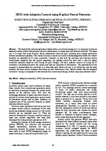
For the system model identification, a random binary noise (RBN) input in the range [& 1 1] was used to excite all the dynamic modes of the system and simultaneously allow for the system steady-state behaviour to be captured. A feedforward neural network of type (4), with 11 hidden neurons with xk ¼ [yk yk&1 yk&2 uk&1]T, W^ 2R1(11 , V^ x 2R11(4 , V^ u 2R11(1 , b^ 2 R11(1 and c^ 2 R was used for modelling purposes, using the Levenberg–Marquardt optimization algorithm. The best neural network parameters !^ that fit the validation data sequences confirmed the good accuracy of the neural network model in capturing the process non-linear dynamics as well as its steady state behaviour. The variance F of !^ was obtained, and a polytopic boundary of Y for the 99% confidence interval was build. The uncertainty region region Y for "! is derived as suggested in } 2, while matrices A1 and B1 are chosen as the Jacobian linearization! in xk ¼ 0, !u"k ¼ 0 of the neural network model: A1 ¼ Fð0, 0, !^Þ 0 and B1 ¼ Eð0, 0, !^Þ. This linearization point can be chosen
Figure 1.
arbitrarily as long as it corresponds to a stable equilibrium point of the system. The set P consists of 64 000 vectors p‘ 2 R30(1 . A polytope P ‘ , enclosing P, is computed using 320 vertices. The steady-state ( ysp, usp) ¼ (0.18, 0.2) corresponds to one of the possible equilibrium points of the identified neural network model and it was chosen differently from the linearization point in order to test robustness of the control algorithm. The robust stabilizing feedback K is then computed according to the procedure described in } 5, with constraints |y| + 0.32 and |u| + 0.8. For Q ¼ I and R ¼ 0.001, the optimal state feedback parameters found were K ¼ [0.0449 & 0.0514 & 0.0174 & 0.6363 0 0]. For an initial condition, y(0) ¼ 0.4, the IOF linearization of the simulated system (31) with the optimal state feedback resulted in the output signal evolution shown in figure 1 a, where the correspondent evolution for the input signal uk, the incremental input !uk and the auxiliary incremental input !uk are plotted in figure 1b. 7. Conclusions This paper presented a procedure which, under some mild assumptions, allows bounded parametric model uncertainties of a feedforward neural network to be propagated through an IOF linearization loop. Based on a polytopic boundary state-space description of the resulting IOF linearized model it was possible to formulate the robust control problem as a convex optimization problem using linear matrix inequalities (LMI). The computation of the additional stabilizing state feedback gives asymptotic tracking on a set point while guaranteeing robust stability with respect to modelling errors. The effectiveness of the approach was shown for a simulation example of a minimum phase benchmark non-linear system. The influence of the controller design parameters on the performance of the closed-loop system is a topic of current research, whose outcome is expected to provide the class of plants under which the proposed solution can be always applicable.
Control performance.
Robust control of dynamical systems Acknowledgement This work was partially supported by program POCTI, from the FCT, Ministe´rio da Cieˆncia e da Tecnologia, Portugal. References Aoyama, A., Doyle III, F. J., and Venkatasubramanian, V., 1996, Control-affine neural network approach for nonminimum-phase nonlinear process control. Journal of Process Control, 6, 17–26. Ayala Botto, M., van den Boom, T., Krijgsman, A., and Sa¤ da Costa, J., 1999, Predictive control based on neural network models with I/O feedback linearization. International Journal of Control, 72, 1538–1554. Ayala Botto, M., Wams, B., van den Boom, T., and Sa¤ da Costa, J., 2000, Robust stability of feedback linearised systems modelled with neural networks: dealing with uncertainty. Engineering Applications of Artificial Intelligence, 13, 659–670. Baron, A., 1993, Universal approximation bounds for superpositions of a sigmoidal function. IEEE Transactions on Information Theory, 39, 930–945. Billings, S., and Voon, W., 1986, Circulation based model validity test for non-linear models. International Journal of Control, 4, 235–244. Chao, A. I., 1995, Stability robustness to unstructured uncertainty for nonlinear systems under feedback linearization. PhD thesis, Massachusetts Institute of Technology, USA. Chen, F.-C., and Khalil, K., 1995, Adaptive control of a class of nonlinear discrete-time systems using neural networks. IEEE Transactions on Automatic Control, 40, 791–801. Cybenko, G., 1989, Approximation by superpositions of a sigmoidal function. Mathematics of Control Signals and Systems, 2, 303–314. Fang, Y., and Kincaid, T. G., 1996, Stability analysis of dynamical neural networks. IEEE Transactions on Neural Networks, 7, 996–1005. Funahashi, K., 1989, On the approximate realization of continuous mappings by neural networks. Neural Networks, 2, 183–192.
1789
Haykin, S., 1994, Neural Networks: a Comprehensive Foundation (New York: Macmillan College Publishing). Hunt, K., Sbarbaro, D., Z_ bikowski, R., and Gawthrop, P., 1992, Neural networks for control systems – a survey. Automatica, 28, 1083–1112. Isidori, A., 1989, Nonlinear Control Systems: An Introduction, Communications and Control Engineering Series (Berlin: Springer-Verlag). Kothare, M., Balakrishnan, V., and Morari, M., 1996, Robust contrained predictive control using linear matrix inequalities. Automatica, 32, 1361–1379. Levin, A. U., and Narendra, K. S., 1993, Control a nonlinear dynamical systems using neural networks: Controllability and stabilization. IEEE Transactions on Neural Networks, 41, 192–206. Lewis, F. L., Yesildirek, A., and Kai, L., 1996, Multilayer neural-net robot controller with guaranteed tracking performance. IEEE Transactions on Neural Networks, 7, 388–399. Narendra, K. S., and Mukhopadhyay, S., 1994, Adaptive control of nonlinear multivariable systems using neural networks. Nerual Networks, 7, 737–752. Narendra, K. S., and Parthasarathy, K., 1990, Identification and control of dynamical systems using neural networks. IEEE Transactions on Neural Networks, 1, 4–27. Seber, G., and Wild, C., 1989, Nonlinear Regression (New York: Wiley). Sjo«berg, J., 1995, Nonlinear black-box modeling in system identification: a unified overview. Automatica, 31, 1691–1724. Suykens, J., Vandewalle, J, and de Moor, B., 1996, Artificial Neural Networks for Modelling and Control of Non-linear Systems (Boston, MA: Kluwer Academic Publishers). Tanaka, K., 1996, An approach to stability criteria of neuralnetwork control systems. IEEE Transactions on Neural Networks, 7, 629–642. van den Boom, T., 2000, Algorithm for low-order polytope approximations. Internal report TvdB:005, System and Control, Faculty ITS, TU Delft.