Robust Localization in Wireless Sensor Networks through the ...

1

Robust Localization in Wireless Sensor Networks through the Revocation of Malicious Anchors Satyajayant Misra† , Guoliang Xue† and Aviral Shrivastava† Abstract— In a wireless sensor network (WSN), the sensor nodes (SNs) generally localize themselves with the help of anchors that are pre-deployed in the network. Time of Arrival (ToA) is a commonly used mechanism for SNs localization in WSNs. In ToA, the SNs localize themselves using the positions of the anchors and the time difference between the receipt of a radio and ultrasound signal transmitted by each anchor. In this setting, the localization process has a high risk of being subverted by malicious anchors that lie about their position and/or distance from the SNs. In this paper, we propose an efficient scheme that helps identify and revoke these malicious anchors. We use a mobile verifier (MV) that moves throughout the network, in some pre-determined manner, and obtains multiple location references from each anchor. For each anchor, the MV tests the mean and the variance of the collected sample to identify if the anchor is malicious. We show through simulations that our scheme successfully identifies more than 80% of malicious anchors with less than 60 references from each. Also, the percentage of false positives is close to 0.

I. I NTRODUCTION Large scale distributed wireless sensor networks (WSNs) have become popular in both the military and civilian domains because of their infrastructureless nature and relative ease of deployment [1]. However, there still exist many fundamental problems that need to be addressed [7]. The problem of robust localization of the wireless nodes is one such fundamental problem in a WSN. Accurate localization is also very important because most applications require the position of the source of the data for effective utilization. In an infrastructureless WSN, for cost effectiveness, not all nodes are equipped with self-localizing abilities. Most sensor nodes (SNs) localize themselves using the position estimates of a group of nodes in the network called the anchors [10], [11], [13]. The anchors are fixed wireless nodes that know their own positions accurately, either through GPS or from pre-programmed information. In this paper, we assume that Time of Arrival (ToA) [15], [13] is the underlying mechanism used for localization. Following the ToA method, each anchor ai periodically broadcasts its identifier (ID) and position information in its neighborhood, as a radio signal (RS) and an ultrasound signal (US) at the same instance of time. We denote these This research was supported in part by ARO grant W911NF-04-1-0385 and NSF grants CNS-0524736 and CCF-0431167. The information reported here does not reflect the position or the policy of the federal government. † All three authors are with the Department of Computer Science and Engineering, Arizona State University, Tempe, AZ 85287-8809. Email: {satyajayant, xue, aviral.shrivastava}@asu.edu.

two components together as the location reference. On receipt of the location reference li from ai , each sensor node (SN) u, calculates the time difference in receipt of the signals and uses the constants, speed of light (c) and sound (s), to obtain an estimate dî of its distance (di ) from ai . The calculation of the estimate dî is given below by Equations 1 and 2 as, ∆t = dî /s − dî /c, 1 , dî = ∆t · 1/s − 1/c

(1) (2)

where ∆t refers to the difference in time between the receipt of the RS and the US. We note that the wireless medium is inherently error-prone, hence the value of ∆t is inaccurate. This results in a SN u being able to obtain only an estimate of di . When u gets a sufficient number of location references from anchors in its vicinity it can use them to estimate its own position. The estimation can be done using the Minimum Squared Error (MSE) (also referred to as the minimum mean square error) method [15], [10] given by, f = min

n X i=1

(k u ˆ − ai k − dî )2

(3)

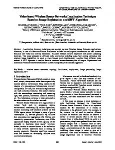
where u ˆ is an estimate of the real position u = (ux , uy ) of u, ai = (aix , aiy ) is the position of anchor ai , dî is the estimate of the distance of ai from u calculated by u using the ToA method, and k · k is the Euclidean norm. n is the number of anchors from whom u receives the localization information. In the absence of measurement ˆ − u k= 0. errors, u ˆ is the correct estimate, that is, k u In the presence of measurement errors, the error in u ˆ is dependent on the measurement error. In this scenario, accurate localization is fairly complex as it is difficult to bound the estimation error. Given the complexity in accurate localization, the presence of malicious lying anchors makes accurate localization significantly more difficult to achieve. We demonstrate this with simulation results. Problem Motivation: In our simulation set-up, each malicious (lying) anchor lied such that its distance from a SN in its range is between [d, d·(1+)], where d is the real distance and = 0.5. Figure 1(a) shows the average of the square of the error (Serr ) in localization over 20 iterations, when lying anchors are included in the localization process. Figure 1(b) shows Serr when the lying anchors are not included in the localization process. We would like the reader to note the

2

Square of error in localization

80

II. R ELATED W ORK

70 60 50 40 12 anchors 11 anchors 10 anchors 9 anchors 8 anchors 7 anchors

30 20 10 0 0

1

2

3

4

5

6

Number of lying anchors

7

8

Square of error in localization

(a) Malicious anchors included in localization 3 2.8 2.6 2.4 2.2 2 1.8 1.6 1.4 1.2 1 0.8 0.6 0.4 0.2 0 0

12 anchors 11 anchors 10 anchors 9 anchors 8 anchors 7 anchors

1

2

3

4

5

Number of lying anchors

6

7

8

(b) Only true anchors used for localization Fig. 1.

Localization error in MSE method

difference in scale of the Y-axis in the two figures and point out that the value of Serr when the number of lying anchors is 0 is the same in both cases. It is easy to see that the error in localization when malicious anchors are included is an order of magnitude higher than when the localization is done with only the true anchors. For instance, when there are 10 anchors in the range of a SN and 5 of them are malicious, the inclusion of malicious anchors in localization results in a value of Serr > 50 sq.m. However, when localization is done without the malicious anchors, the value of Serr < 0.8 sq.m. Thus, we can conclude that the presence of malicious anchors is detrimental to accurate localization and their revocation is necessary in the interest of increasing the accuracy. In this paper, we propose a technique for identifying and revoking the malicious anchors.We use a mobile verifier (MV), sent by the base station (BS), that obtains location references from the anchors and identifies the malicious ones by performing statistical analyses of the location references. The malicious anchors, once identified, can be revoked from the network, to prevent subversion of localization. Using our technique we could successfully identify and revoke more than 80% of the malicious anchors in the network using only 60 references from each anchor. In Section II, we present the related work. In Section III, we present the system and threat models along with their assumptions. Section IV presents our proposed mechanism, while Section V presents the simulation results. We conclude our paper in Section VI.

Localization schemes in WSNs may be classified as range-based or range-free. The range-based mechanisms, as proposed in [3], [16], [10], [5], perform localization by measuring properties such as point-to-point distance or angle estimates, whereas the range-free localization mechanisms as proposed in [8], [9], [11], [6], [15] do not require any physical measurements to perform localization. These mechanisms may use hop count or area-based estimation to localize a node [6]. Generally, range-based mechanisms lead to more accurate localization; however, they tend to be resource intensive and may require specialized hardware [16], [13]. The method used for position estimation is either based on minimum mean/median square estimation [15], [10], convex programming [4], [2], or triangulation [16]. There are many schemes, such as [5], [16], [10], [11], [8], [9], [11] that have been proposed to increase security and robustness of localization by either performing secure localization, doing location anomaly detection, or through location verification. Accurate localization in the presence of malicious anchors transmitting erroneous estimates has been dealt with by Li et al. [10], Liu et al. [11], and Du et al. [5]. In [10], [5], the schemes attempt to identify the anomaly and perform compromise resistant localization, whereas [11] attempts to detect and remove the malicious anchors from the network. However, the performance of the above schemes is severely limited in the presence of a large number of malicious anchors which may or may not be colluding. In this paper, we propose a novel scheme that can identify a large proportion of the malicious anchors even when the majority of the anchors in the network are malicious and colluding. Infact even when all the anchors are lying they can be identified. This is possible because each anchor is verified independently, and hence the results of the verification of an anchor cannot be influenced by another. III. S YSTEM M ODEL

AND

A SSUMPTIONS

The system model used for our proposed technique is given below: • The network consists of a set of anchors A = {a i , i = 1, . . . , n} and a set of sensors S = {si , i = 1, . . . , n} that are deployed randomly and are fixed after deployment. • Each anchor ai knows its own position ai (ai = (aix , aiy )). • The transmission range of the SNs is r and the anchors is R (R ≥ r > 0), while the reception range of the MV is ≥ R. • The anchors are equipped with radio/ultrasound transmitters and can transmit both signals simultaneously. • The anchors broadcast their location references periodically.

3

•

•

•

•

•

•

The SNs and the MV are equipped with both radio and ultrasound receivers. The Mobile Verifier (MV) is GPS enabled and can obtain its own position accurately. Localization is required throughout the network’s lifetime to localize new SNs added to the network. ˜ the measurement error, is distributed normally, n˜ v n, N (0, σ02 ), with domain x ∈ [−δmax , δmax ]. Thus, the probability P r[n < −δmax ] = P r[n > δmax ] = 0. If f (x) is the probability density function for a random variable x ∼ N (0, 1) then σ02 is given by, R −δmax 2 x f (x)dx δmax 2 σ0 = (4) R −δmax R∞ 1 − −∞ f (x)dx − δmax f (x)dx The anchors transmit their references encrypted using a key from a hash chain. The key is released at a later time instant (delayed key disclosure mechanism). This is similar to the mechanism of µTESLA [14]. All devices have omnidirectional antennas.

A. Assumptions •

• •

We assume that the anchors lie such that the resulting distance estimate is proportional to their actual distance from a SN. The proportion is a uniform random variable ∼ U [−max , max ], where max is a constant. No two anchors have the same position in the network. The anchors have enough memory and computation abilities to generate and store hash chains of the keys.

B. Threat Model and Security Assumptions We assume that the malicious anchors may be compromised by a powerful external adversary to lie about their distance references. Also, the MV is assumed to be uncompromisable by an adversary. The MV could be a mobile vehicle or a human operator. In this subsection, we use ai to illustrate a malicious anchor. The use of delayed key disclosure by the anchors for transmitting their location references ensures that malicious anchors in the neighborhood cannot change or replay the references. In addition, a malicious anchor ai cannot revoke a true anchor aj by masquerading as aj and broadcasting false location references. Our scheme is not affected by wormhole attacks. The MV can successfully identify wormhole attacks. For instance, if ai replays the location information of some other anchor aj not in the neighborhood, the MV can identify that aj does not belong to the neighborhood by analyzing the location references of aj . In addition, ai can also be identified as the source of the message, since the MV can estimate the position ai from any 4 location references. We would like to note here that in ToA 4 references are required to estimate the position of a node [15]. In this setup, there are only three possible mechanisms by which a malicious anchor can subvert accurate localization,

namely by lying about its position, its distance (by not transmitting the RS and the US simultaneously), or by lying both ways. If malicious anchor ai lies about its position so that the position changes but its ID remains same, then it can be easily caught by the SNs themselves. However, if ai uses a set of IDs, then the SNs will not be able to identify such an attack. This kind of attack can be identified by the MV. If the MV obtains 4 readings for each of the IDs used by ai , it can easily estimate the location of the source (ai ) and thus identify that the source of all the localization messages with different IDs to be ai . Once ai is identified it may be revoked. If ai lies by sending the RS and US at different times it could successfully cause distance reduction (US is sent earlier than the RS) or enlargement (US is sent later than the RS) attacks. Owing to the uncertainties due to measurement errors, this attack is difficult to identify by simply checking a few location references from a malicious anchor. Our technique identifies the malicious anchors in this scenario. The technique can also identify ai , if it lies about its position and distance simultaneously (or even its position only). The reasons for the applicability of our scheme for all three scenarios is presented in the next section. We note here that distance enlargement/reduction attacks may also be caused by denial of service attacks. This kind of attack may be prevented by using error correcting codes or spread spectrum techniques described in literature [17]. We do not consider this attack in our threat model. IV. D ESCRIPTION

OF THE

S CHEME

The MV is sent into the network by the Base Station (BS). The MV can be sent into the network any number of times. Each instance that the MV enters the network and returns to the BS is termed an iteration. In each iteration the MV obtains a constant number of location references (K) from each anchor. K is a tunable system parameter which is dependent on the amount of energy required by the MV to obtain K references from each anchor, the amount of energy at the disposal of the MV, and also the desired level of accuracy. The MV may be recharged on getting back to the BS. In order to identify malicious anchors with high confidence, a MV has to obtain at least a certain number of location references from each anchor (derived later). The number of iterations is dependent on the total number of references required and the value of K. For our technique to be robust and efficient we need to address the following four questions, namely: • How to ensure that all anchors are covered by the MV? • How to make the route of the MV in the network appear random to an outside observer? • How to perform statistical testing on the location references obtained from each anchor? • How to revoke the anchors identified as malicious?

4

We overlay√the network with a virtual grid (Gr) of squares of side R/ 2, where R is the reception range of the MV. Each square in the grid is defined as Sxy where x and y are the X-coordinate and Y-coordinate of the lower left corner of the square. The network may be represented by a graph G(V, E), where V = {Sij : Sij is a square in Gr} ∪ BS, BS is the position of the BS, and E = {(Sij , Skl ) : Sij and Skl are adjacent}. We note T here that two vertices Sxy and Sab are adjacent iff Sxy Sab 6= φ, for the squares Sxy and Sab . In each iteration, the MV visits all the squares before returning to the BS, thus covering all the anchors. A. Setup of the paths of the MV The MV collects data passively in the network, thus its chance of getting detected is small. However, it is still possible for a strong external adversary to identify the presence of the MV in the network and learn its path. If the MV follows the same path in the network for each iteration, from the current position of the MV in a square Sij , the adversary can identify the subsequent squares the MV will visit. It can then direct the malicious anchors in those squares to transmit correct location references during the time period that the MV is in range, thus making malicious anchors identification ineffective. So, it is desirable that for each iteration the MV follows a different path from the previous iterations. But, due to the limited number of paths repetitions are unavoidable. However, we note that repetition of a path should be infrequent and also the paths used for a given number of successive iterations should differ as much as possible. This makes it difficult for the adversary to predict the position of the MV. In our scheme, for each iteration, Q the MV chooses a path from an ordered sequence of paths = {π1 , π2 , . . . , πm } that is pre-computed at the BS and stored in the MV. Each path πi , i = 1, . . . m, is defined as a sequence πi = {BS, Skl , Sqr , . . . , BS} of vertices of G(V, E) where any two adjacent vertices in the sequence form an edge. For the first iteration, the MV chooses π1 , for the second π2 , and so on. When all the paths are used up, they are all available for selection again, and Q the procedure is repeated. For any two paths πi and πj in we define a score function, F(πi , πj ) = |{(Skl , Sqr )|(Skl , Sqr ) ∈ πi and πj }|. A smaller value of F(πi , πj ) is desirable as it means that the difference between Q πi and πj is greater. The ordered sequence of paths = {π1 , π2 , . . . , πm } is chosen by the BS such that for some given p < m the function, i+p m−p X X i=1 j=i+1

F(πi , πj )

(5)

is minimized. That is, for a path πi ∈ Π the sum of the score functions corresponding to the next p paths in Π is minimized, hence these p paths satisfy the desirable property of being as different from πi as possible, given a maximum

possible choice of m − 1 paths. This procedure is performed at the BS offline. B. Setup for Hypothesis Testing To test if an anchor is malicious, the MV performs hypothesis testing for the mean (µ) and the variance (σ 2 ) of the location references. As described before, the measurement error is given by n˜ ∼ N (0, σ02 ), where σ02 is given by Equation 4. The estimate of the distance of an anchor ai from the MV can be modeled as dî = di · (1 + δi ), where δi is the measurement error coefficient (∼ N (0, σ02 )). In the event that ai is true, the calculated distance dcalc satisfies i Equation 6, dcalc =k m − ai k= di , (6) i where m is the position of the MV. Hence the expression, dî /dcalc − 1 = δi , i

(7)

which is the coefficient for the measurement error. From the statistical perspective, given a sample of location references of an anchor ai , if ai is true, the mean and the variance of the error should be close to the values 0 and σ02 respectively. For a malicious anchor ai , Equation 7 will not hold, as it may lie either about its distance or its position. As a result there would be a greater variance in the error coefficient δi and also a deviation in the mean µi . We note that a sample variance greater than σ02 , or a shift in the sample mean, or both may be observed if ai lies. This is irrespective of how ai lies (position only, distance only, or both), as either dî , or dcalc , or both shall be affected by the lie. The i tests we propose would be able to identify the malicious anchors using the above facts. For brevity, we illustrate the statistical tests for only the case where the anchors lie about the distance. However, the tests are applicable to identify anchors that are lying in the other ways mentioned. From the location references obtained for each anchor ai , we perform statistical hypothesis tests for the mean and the variance of the error coefficients. For more information about the theory of hypothesis testing we refer the reader to [12]. 1) Hypothesis testing for mean: The hypothesis test for the sample mean µ is given by, H0 : µ = 0 versus H1 : µ 6= 0.

(8)

We know that the mean of the distribution is µ = 0. A malicious anchor ai may lie such that the mean (µi ) of the resultant error coefficients is non-zero. This malicious anchor can be identified if the null hypothesis of the above test is rejected. For the tests, we denote the probabilities for Type I error and Type II error by the standard variables α and β [12]. The power of the test, defined as the probability of rejecting the null hypothesis H0 when H1 is true, is given by 1−β. Hence, lower the value of β higher is the power of ¯ we can obtain the value the test. Given the sample mean X,

5

of the test statistic, Z0 =

¯ X−0 √ , σ/ (N )

which is ∼ N (0, 1).

We would reject H0 if Z0 < −zα/2 or Z0 > zα/2 , where zα/2 is the 100α/2 percentage point of ∼ N (0, 1). And we would fail to reject H0 otherwise. If H0 is rejected it implies that the mean of the error coefficients of ai is in the critical region, which implies that ai is lying. It is easy to see that with an increase in the sample size N the accuracy of the test increases. However, this requires the MV to spend more time in each square Sxy . Hence, there exist trade-offs between the accuracy we require and the amount of time and energy required to attain such an ¯ − µ, the size accuracy. For given values of α, β, and δ = X of the sample (N ) required to produce the desired Type (z +z )2 ·σ 2 I and Type II errors is given by N = α δβ2 [12]. The value of β defines the probability of a false negative, higher the value of β less powerful is the test, hence lower is the probability of rejecting H0 . For higher values of β, the tests can be performed for smaller values of N , but with the chance of increase in false negatives. However, we believe that false negative is not as serious as having false positive. A lying anchor that is not caught because of the lower power of the test owing to a small sample size can be caught subsequently with increasing sample size. On the other hand, false positive is highly undesirable as it may result in the anchor being incorrectly identified as malicious, hence resulting in its revocation. Thus in our tests we limit the Type I errors by using a high value for α. Algorithm 1 Algorithm followed by MV in an iteration 1: INPUTS: Path πp ∈ Π for iteration p and Kp (no. of references required per anchor); 2: OUTPUTS: List of malicious anchors in network; 3: Start at the BS; 4: repeat 5: numRefs ← 0; 6: Move to the next vertex Sij ∈ πp ; 7: while numRefs != Kp do 8: Choose at random position Px,y ∈ Sij ; 9: Get a reference for each anchor al ∈ Sij ; 10: numRefs++; 11: mark Sij visited; 12: end while 13: until all Sij ∈ πp are visited. 14: for all anchors al do 15: totalRefsp ← totalRefsp−1 + Kp ; {add the Kp references of al to ones from previous iterations} 16: Do hypothesis testing on µ and σ 2 (Section IV-B); 17: if al fails either tests then 18: Add al to malicious list; 19: end if 20: end for 21: Transmit malicious list to BS;

2) Hypothesis testing for the variance: At first, we present the motivation for performing hypothesis testing for the variance. Consider a malicious anchor ai , let the distance 0 estimate of ai from the MV be given as dk for the kth reference in an iteration, and let the real distance be dk . Let 0 us consider that ai lies such that dk = dk ·(1+(−1)k ·) for reference k = 1, . . . , K, where (> 2 · δmax ) is a constant error coefficient. In this case, despite ai lying by a significant ¯ ≈ 0, since the measurements alternate between amount, X two high extremes about µ = 0. Thus ai would not be caught despite lying significantly. This shortcoming can be remedied by testing the sample variance. The hypothesis testing on the sample variance σ 2 is given by, H0 : σ 2 = σ02 versus H1 : σ 2 > σ02 .

(9)

In the above example, if we perform a hypothesis test for the variance, ai would be caught. The null hypothesis H0 would be rejected as the variance of the sample obtained from ai would be >> σ0 . For a sample of size N , we can define the test statistic s2 2 , where sˆ2 is the sample variance. X02 X0 = (N −1)·ˆ σ02 follows the chi-square distribution χ2 with N − 1 degrees of freedom denoted by χ20,n−1 . Hence, the null hypothesis H0 is rejected if χ20,n−1 > χ2α,n−1 where χ2α,n−1 is the upper 100α percentage points of the χ2n−1 distribution. If H0 is rejected then sˆ2 is in the critical region, hence the corresponding anchor is identified as malicious. Algorithm 1 presents the operation of the MV in the network during a typical iteration. Once the MV gets the references from all the anchors, it performs the hypothesis test on the combined sample (from previous iterations and current iteration) to identify the malicious anchors. To prevent old references from biasing the effect of new references they need to be removed at suitable intervals. Identifying such an interval of optimum size is a future work direction. The list of malicious anchors and their positions is broadcast by the BS as a revocation message in the network. The revocation messages for the SNs is authenticated by the BS using the µTESLA mechanism. V. S IMULATION R ESULTS The WSN is deployed in a square field of dimensions 100 × 100 sq. units. This field is overlaid with a grid of squares of 20 × 20 sq. units. In each square, 10 anchors are deployed randomly. The transmission range of the anchors is set to 30m and the location reference broadcast period is set to 1 second. The maximum error coefficient was chosen to be |δmax | = 0.2, the corresponding σ02 = 0.033 and σ = 0.182; α = 0.01 and β = 0.1. Figure 2(a) shows the percentage of malicious and true anchors caught by the hypothesis test for µ, given 3, 5, or 7 malicious anchors per square. The proportion of lie in the localization reference for each malicious anchor ai was chosen to be ∼ U [−0.2, 0.4]

1 0.8 false anchors (3 per sq.) false anchors (5 per sq.) false anchors (7 per sq.) true anchors (3 per sq.) true anchors (5 per sq.) true anchors (7 per sq.)

0.6 0.4 0.2 0 20

40 60 80 100 120 Number of references per anchor

Percentage of malicious anchors caught

Percentage anchors caught

6

Hence our proposed technique can identify a large percentage of the malicious anchors in the network, thus improving the accuracy of SN localization.

1

0.8

0.6 µ = 0.15 m

0.4

µm = 0.2 µ = 0.25 m

0.2

140

20

1

0.8 false anchors (3 per sq.) false anchors (5 per sq.) false anchors (7 per sq.) true anchors (3 per sq.) true anchors (5 per sq.) true anchors(7 per sq.)

0.6 0.4 0.2 0 20


(c) Test for σ 2

140

(b) Test for µ

140

Percentage of malicious anchors caught

Percentage anchors caught

(a) Test of µ


1

VI. C ONCLUSIONS AND F UTURE W ORK In this paper, we propose a scheme that successfully identifies a large number of malicious anchors that may subvert the localization process in a WSN. In the future, we would like to find improved solutions for finding untraceable paths in the network and also study improvements in the energy requirements of the technique.

0.8

R EFERENCES

0.6 |ε

| = 0.2

|ε

| = 0.3

max

0.4

max

|εmax| = 0.4

0.2

|ε

| = 0.5

max

0 20


140

(d) Test for σ 2

Fig. 2. Simulation results. 2(a) and 2(c): Tests for µ and σ 2 with 3, 5, or 7 malicious anchors per square. 2(b) and 2(d): Percentage of malicious anchors caught for different proportions of lie.

thus having mean µm = 0.1. The top three curves represent the number of malicious anchors caught, while the bottom three curves represent the number of true anchors caught (false positives). Even with as few as 20 location references more than 70% of the malicious anchors are caught. As expected, with the increase in number of references more malicious anchors are caught. More than 90% malicious anchors were caught when the number of references were 60 or more. Also, the percentage of anchors caught is independent of the number of anchors in a square. We wish to point out that due to the low value of α(= 0.01) the percentage of false positives is close to 0 in our scheme. As a result, just 20 or more references result in almost no false positives. Figure 2(b) shows the percentage of malicious anchors caught for different values of the mean µm of the malicious anchors. As the anchors lie more, a greater number of the malicious anchors are caught with a lesser number of references. Even for a low value of µm = 0.15, our technique can catch more than 80% of the malicious anchors with as low as 40 location references. Thus, even with a small number of references the malicious anchors can be easily identified. Figure 2(c) shows the results for the test for σ 2 . Similar to the test for µ, the false positives are low and the the number of malicious anchors caught increases with an increase in the number of references, with greater than 80% caught for the 60 or more references. Figure 2(d) shows the percentage of anchors caught with increasing lie coefficients. As the anchors lie more, more of them are caught with higher accuracy. This is desirable for both the test for mean and variance, as anchors that lie more are more harmful for the localization process.

[1] I. Akyildiz, W. Su, Y. Sankarasubramaniam, and E. Cayirci. Wireless sensor networks: A survey. Computer Networks, 38(4):393–422, 2002. [2] Pratik Biswas, Tzu-Chen Lian, Ta-Chung Wang, and Yinyu Ye. Semidefinite programming based algorithms for sensor network localization. ACM Transaction on Sensor Networks, 2(2):188–220, 2006. [3] Xiuzhen Cheng, Andrew Thaeler, Guoliang Xue, and Dechang Chen. TPS: A time-based positioning scheme for outdoor wireless sensor networks. In Proceeding of Joint Conference of the IEEE Computer and Communications Societies (INFOCOM ’04), volume 4, pages 2685–2696, 2004. [4] L. Doherty, K. Pister, and L Ghaoui. Convex position estimation in wireless sensor networks. In Proceedings of the IEEE INFOCOM, pages 22–26, 2001. [5] W. Du, L. Fang, and P. Ning. LAD: Localization anomaly detection for wireless sensor networks. In Proceedings of the 19th IEEE International Parallel and Distributed Processing Symposium (IPDPS), 2005. [6] Tian He, Chengdu Huang, Brian M. Blum, John A. Stankovic, and Tarek F. Abdelzaher. Range-free localization and its impact on large scale sensor networks. Trans. on Embedded Computing Sys., 4(4):877–906, 2005. [7] C. Karlof and D. Wagner. Secure routing in wireless sensor networks: Attacks and countermeasures. Elsevier’s Ad Hoc Networks Journal, Special Issue on Sensor Network Applications and Protocols, 1(2– 3):293–315, September 2003. [8] L. Lazos and R. Poovendran. HiRLoc: High-resolution robust localization for wireless sensor networks. IEEE Journal on Selected Areas of Communications, 24(2):233–246, February 2006. ˘ [9] L. Lazos, R. Poovendran, and S. Capkun. ROPE: Robust position estimation in wireless sensor networks. In Proceedings of Information Processing in Sensor Networks (IPSN), pages 324–331, 2005. [10] Z. Li, W. Trappe, Y. Zhang, and B. Nath. Robust statistical methods for securing wireless localization in sensor networks. In Proceedings of Information Processing in Sensor Networks (IPSN), pages 91–98, 2005. [11] D. Liu, P. Ning, and W. Du. Detecting malicious beacon nodes for secure location discovery in wireless sensor networks. In Proceedings of the 25th IEEE International Conference on Distributed Computing Systems (ICDCS), pages 609–619, 2005. [12] D. Montgomery and G. Runger. Applied Statistics and Probability for Engineers. John Wiley and Sons Inc., 2002. [13] D. Niculescu and B. Nath. Error characteristics of ad hoc positioning systems (APS). In Proceeding of ACM MobiHoc, 2004. [14] A. Perrig, R. Canetti, D. Tygar, and D. Song. The tesla broadcast authentication protocol. Cryptobytes, 5(2):2–13, 2002. [15] A. Savvides, C. Hans, and M. Srivastava. Dynamic fine-grained localization in ad-hoc networks of sensors. In Proceeding of ACM MobiCom, pages 166–179, 2001. ˘ [16] S. Capkun and J. Hubaux. Secure positioning in wireless networks. IEEE Journal on Selected Areas of Communications, 24(2):221–232, February 2006. [17] A. Wood and J. Stankovic. Denial of service in sensor networks. IEEE Computer, 35(10):54–62, oct 2002.